Abstract
The optimal operation of a hybrid AC-DC microgrid is investigated in this study. The operation of an AC microgrid connected to the main grid and an islanded DC microgrid has been examined under three management approaches. In the first approach, two microgrids are not connected, and the DC microgrid is operated in the islanded mode. In the second and third approaches, AC and DC microgrids are connected. The main difference between these two approaches is the energy management framework. In the second approach, each microgrid has its own management system, while the third approach integrates both into a single energy management system to form an AC-DC microgrid that minimizes overall operational costs. The main goal of the proposed model is to minimize the operating costs of two microgrids over a 24 h period. The investigated AC microgrid includes a microturbine, wind turbine and diesel generator in order to supply the residential load profile, and the DC microgrid includes an energy storage system, fuel cell, wind turbine and solar panel in order to supply the commercial load profile. Simulations are performed first with a wind and load scenario in order to show and compare the optimal points of using the decision variables in three approaches. Finally, in order to prove the effectiveness of the proposed method in the presence of uncertainties, the cost distribution function for the three approaches is presented by means of Monte Carlo simulation. Applying the proposed model results in the following the cost reduction: 67.9% in the DC microgrid, 14.2% in the AC microgrid and 24.4% overall. This reduction is primarily attributed to the microgrid central energy management system, which decreases reliance on the main grid and instead utilizes alternative sources such as fuel cells. Comparing the first and third approaches, the fuel cell’s contribution to supplying microgrid loads increased by 29%, while the main grid’s participation decreased by 26%.
1. Introduction
A microgrid is a collection of programmable and unprogrammable generation sources and some loads that are supplied by these sources [1]. Another important element in a microgrid is the battery that is used to supply the loads [2]. Over the past years, the use of microgrids has increased due to its technical [3] and economic [4] advantages. These benefits are related to reducing power losses [5], increasing voltage stability [6] and loadability [7], increasing reliability [8], reducing operating costs [9] and reducing emissions [10]. Microgrid operation is performed in two different modes. One mode is grid-connected mode, in which power is provided through the main grid in addition to the available resources [11]. The other mode is islanded mode, where no connection is established to the main network [12]. Also, microgrids can be divided into three categories based on the type of power generation source and load connected to the microgrid. So, microgrids are classified into AC, DC and AC-DC [13]. The use of hybrid AC-DC microgrids achieves the benefits of both microgrids and ultimately improves power quality [14] and increases reliability [15].
Depending on the status of the connection to the main grid and due to the presence of programmable and unprogrammable units and for the different goals of the microgrid owners, there is a fundamental need for accurate management of power generation resources and determining the charging and discharging time of energy storage systems [16]. The task of the microgrid management system is to coordinate the microgrid units according to the user’s goals [17]. Coordination between units means determining the optimal operating points of programmable units according to the generation capacity of non-programmable units, in order to reliably supply the available loads in the microgrid, within the framework of the investigated approach [18].
Proper energy management and reliable operation in microgrids are some of the important challenges in the operation of microgrids, and for this purpose, there are different methods that have been presented in various studies. In this section, some of these studies are reviewed in detail. In [19], energy management in the microgrid is discussed, aiming at minimizing operation costs. Also, numerous constraints, including the power balance, generation capacity, consumer loads and dynamic performance of energy storage systems are considered. This is accomplished using the intelligent Golden Jackal Optimization algorithm, and the results are compared with other optimization algorithms such as particle swarm optimization (PSO), Tabu Search and Artificial Bee Colony. In [9], energy management is presented in a microgrid in the islanded operation mode that includes three types of renewable resources (photovoltaic, biomass and geothermal) and energy storage by different algorithms like PSO, a genetic algorithm and Harmony Search. The mentioned method is aimed at reducing costs, and the uncertainty related to weather conditions is also considered. In [20], an energy management model is presented to predict the production values of wind and solar resources. The objectives are to reduce the cost of power consumption and cost of battery degradation, and the proposed method is implemented using a multi-objective genetic algorithm. In [21], the optimal economic operation of a microgrid without an energy storage system and then in the presence of an energy storage system is presented. The results show that the system operation is more flexible in the presence of batteries, and the positive economic impact of this approach is visible.
In [22], an energy management system is used in a hybrid AC-DC microgrid with the aim of reducing operation costs. In this work, the stability of the network frequency is guaranteed considering the uncertainty issues. Optimal energy management in microgrids is a challenge. In [23], a practical method is presented for energy management in a hybrid AC-DC microgrid with the machine learning technique. The mentioned method consists of two parts: forecasting and scheduling. In this research, the grey wolf algorithm is used to solve the optimization problem and adjust the setting parameters of the forecasting model. In [24], a method of energy management is presented by the PSO algorithm for effective control in microgrid operation to reduce energy costs in the network. In [25], a method for determining the optimal sizing and reducing the electricity cost is presented for a hybrid microgrid in the islanded mode.
In [26], a method is presented to manage the power of a hybrid AC-DC microgrid in which the grids are considered in different operation modes to reduce the cumulative cost. In [27], an optimal two-stage strategy is presented for power management in a hybrid AC-DC microgrid where the uncertainty of generation resources and load is considered with a robust optimization method.
In [28], an energy trading strategy for AC-DC hybrid microgrids in the presence of distributed generators and energy storage systems is presented. The proposed strategy goal is the reduction in the operating cost of each microgrid. The proposed framework allows each microgrid to schedule its economical and reliable operation by optimizing its resources as well as exchanging power with other microgrids and the main grid. In [29], a stochastic mixed-integer nonlinear programming model is presented, and it is linearized to a mixed-integer linear programming form. This method is used to optimize the energy–water–carbon relationship in AC/DC microgrids with the aim of sustainable development of a community. The model optimizes the location, and operation of diesel generators, voltage source converters, photovoltaic systems, wind turbines and battery energy storage systems while managing CO2 emissions. In [30], an advanced energy management method for AC/DC microgrids is proposed. The proposed energy management system supports the green transition as it is designed for a microgrid that includes renewable generation, batteries and electric vehicles. A deep-learning-supported non-intrusive load monitoring algorithm is deployed to solve the energy management study.
From the literature review, it is evident that previous studies on microgrid energy management have primarily focused on either AC or DC microgrids individually or as hybrid AC-DC systems. Additionally, energy management systems have either managed microgrids separately or facilitated their integration. However, there is a need for a comprehensive study that evaluates microgrid performance under different connection and management scenarios and compares the resulting outcomes. In this paper, the optimal management and operation of an AC microgrid (ACMG) that supplies the AC residential load and a DC microgrid (DCMG) that supplies the commercial DC load is presented. With the growth of DC sources and loads, the need to investigate and operate DCMGs alongside ACMGs and connect these two types of microgrids to analyze their benefits has become more prominent.
In the proposed method, the economic operation of an ACMG connected to the main grid and an islanded DCMG is investigated under three islanded and connected management approaches. In the first approach, two microgrids are separate and do not exchange power with each other. In the second approach, two microgrids are connected to each other, but each one has its own microgrid central energy management system (MCEMS) for power management and does not have access to the other’s data. This enables the owners of microgrids to be independent in adjusting their decision variables and prioritizing the minimization of the cost of their own microgrid over the minimization of the total cost of two microgrids. In the third approach, two microgrids are considered as a single AC-DC microgrid operating with a common MCEMS. The main goal of this method is to examine the advantages and disadvantages of each approach. The objective function is to minimize the operating costs of the microgrid for the next 24 h by changing the usage type of the MCEMS and the connection between them. The PSO algorithm has been used to solve the problem and find the optimal points of operation. Simulations are first performed with a wind and load scenario in order to show and compare the optimal points of operation and the decision variables in three approaches. Finally, in order to prove the effectiveness of the proposed approaches in the presence of uncertainties, the cost distribution function for the three approaches is presented by means of Monte Carlo simulation. The main contributions are summarized as follows:
- Examining the operational conditions of microgrids when functioning independently or interconnected.
- Analyzing microgrid performance when each AC or DC microgrid has its own central energy management system (MCEMS) versus when a single MCEMS is used.
- Incorporating uncertainty in renewable energy sources and loads across different connection and management scenarios.
- Minimizing microgrid operating costs by optimizing the MCEMS configuration and interconnection strategy.
The structure of this paper is as follows. In Section 1, the introduction and literature review are examined. In Section 2, microgrid structure is presented with three approaches. Section 3 presents the equations and formulation of the problem including cost functions of power generation units, objective functions and decision variables. In Section 4, the results of the simulation will be shown. Finally, Section 5 is devoted to the conclusion.
2. Microgrid Structures
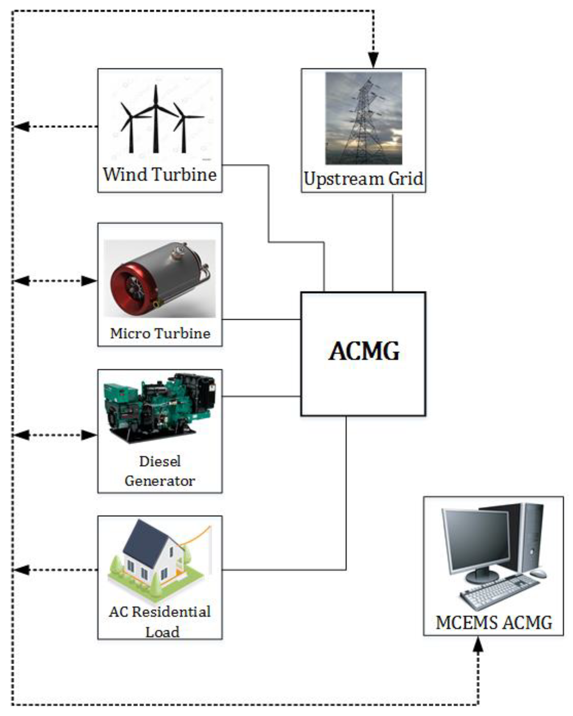
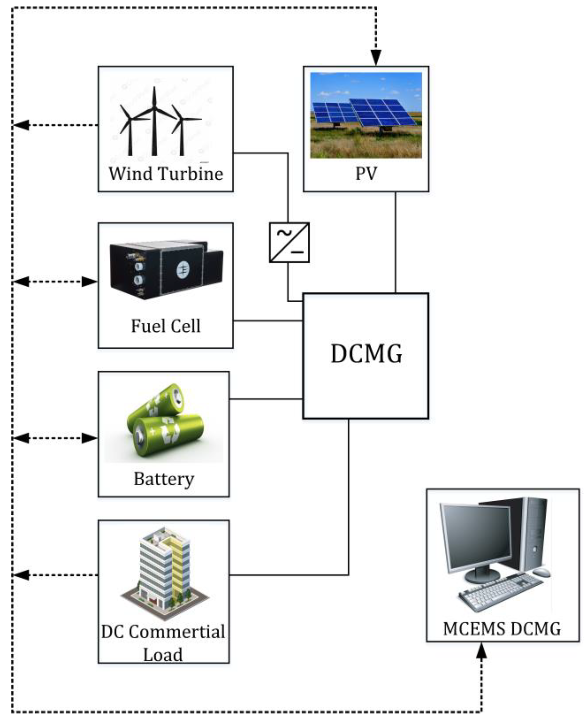
In this section, the structure of the microgrids examined in this work is presented. In the first approach, the microgrids are operated separately. A separate MCEMS for each microgrid is responsible for collecting data related to wind speed, solar radiation and the generated power of renewable units and then calculating the values related to the decision variables according to the load profile and constraints considered in each microgrid. In the DC section, the MCEMS has the ability to adjust the operating points for fuel cell and battery. In the AC section, the MCEMS has access to the output power data from the wind turbine (WT) and the AC load profile to be supplied in the ACMG. In this approach, the MCEMS of the AC section has the ability to adjust the decision variables of the ACMG including the generated power of the diesel generator, the microturbine and the exchanged power with the main grid. The structures of the ACMG and DCMG for the first approach are shown in Figure 1 and Figure 2, respectively.
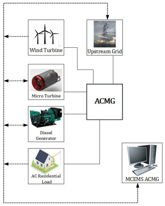
Figure 1.
Structure of the ACMG for the first approach.
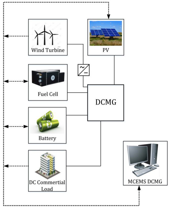
Figure 2.
Structure of the DCMG for the first approach.
In the second approach, the connection between the two microgrids is established by an inverter. From the point of view of the DCMG, the ACMG is considered as the main grid. In order to provide a fair power exchange, the ACMG will exchange power with the DCMG with the rate of the main grid. So, in this approach, another decision variable, i.e., the exchanged power between two microgrids, is added to the DCMG decision variables. According to the power exchanged between two microgrids when the power is transferred from the DC side to the AC side, the MCEMS of the ACMG considers the DCMG similar to an unregulated power generator (a negative load). In addition, the DCMG is considered as a load when it receives power demand. The structure of the microgrids in the second approach considering the connection between the ACMG and DCMG can be seen in Figure 3.
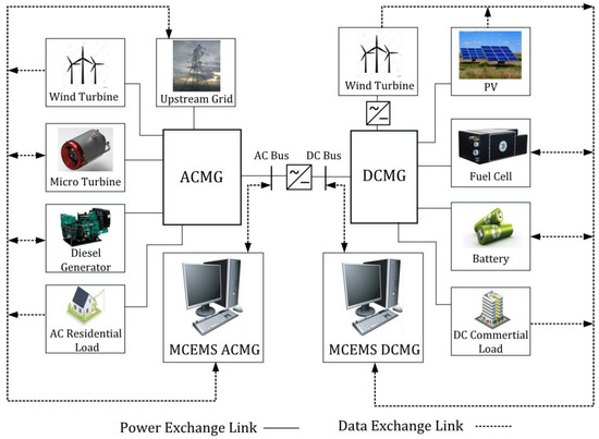
Figure 3.
Structure of the microgrids in the second approach considering the connection between the ACMG and DCMG.
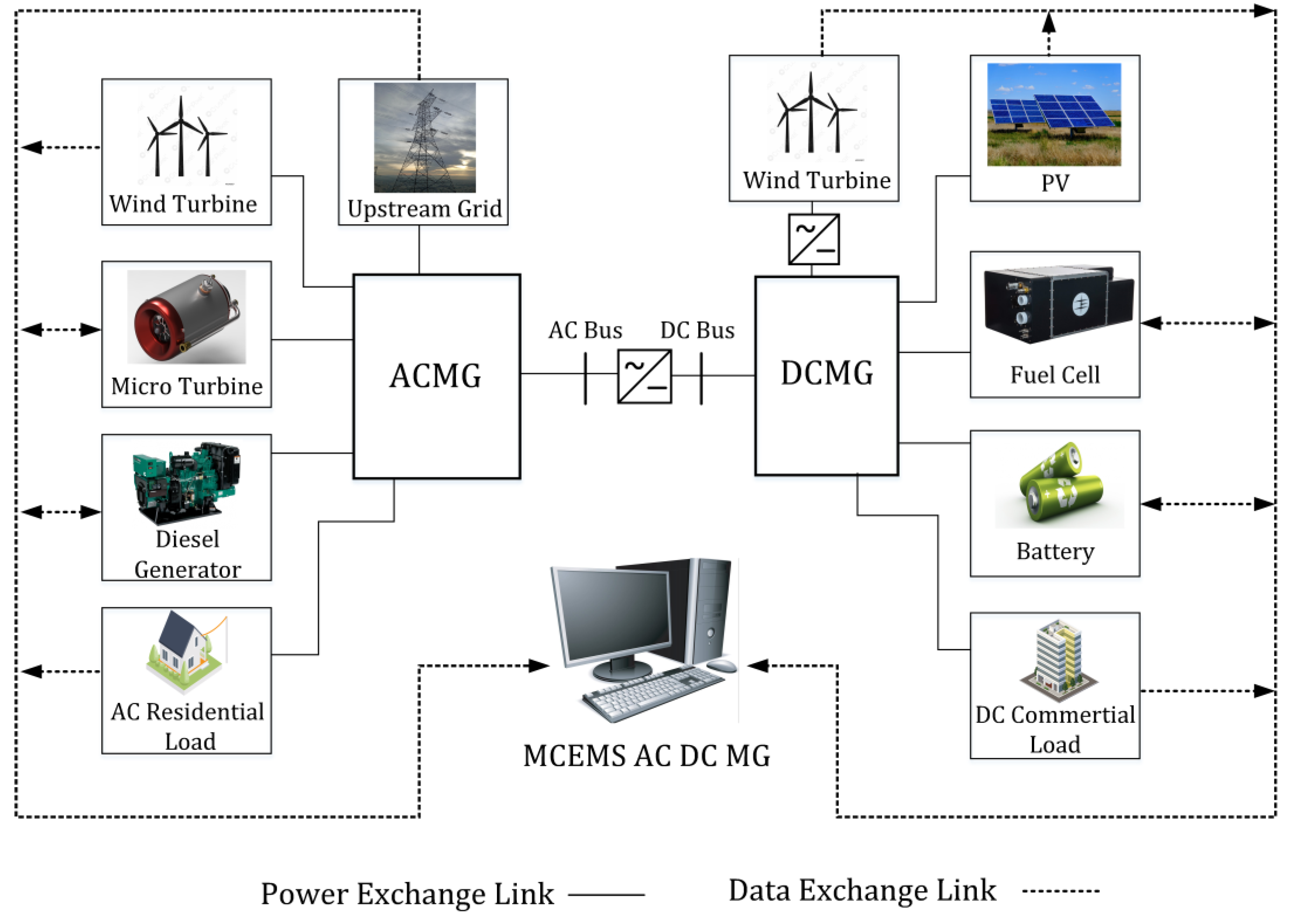
In the third approach, the connection between two microgrids is established by an inverter like in the second approach. The common MCEMS will form the concept of a hybrid AC-DC microgrid by combining two microgrids. In this approach, the generation units of two microgrids work in coordination with each other, and all other units are considered in adjusting their operating points. Battery charging and discharging will be done according to all units and the load profile of two microgrids. In this approach, the concept of two separate owners with the aim of increasing their individual profit for each microgrid is ignored, and the central management system will act according to the increase in the cumulative profit of two microgrids, which has now become one hybrid AC-DC microgrid. The structure of microgrids in the third approach and how they are connected, as well as how data are transferred in the MCEMS, are shown in Figure 4.
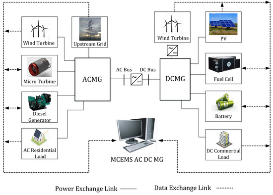
Figure 4.
Structure of the microgrids in the third approach.
The difference between Figure 3 and Figure 4 lies in the performance and management system of the ACMG and DCMG. In Figure 3, the two microgrids operate independently, with power exchange being the only interaction between them. Each microgrid has its own dedicated management system, prioritizing its own profits without considering the benefits of the other microgrid. In contrast, Figure 4 depicts a hybrid microgrid, where the two microgrids are interconnected and managed by a unified power management system. In this setup, the operation of each component is optimized to maximize the overall profitability of the entire microgrid. For example, in Figure 3, the battery power is used exclusively to compensate for power shortages within the DCMG. However, in Figure 4, although the battery is physically located in the DCMG, it can also be utilized to address power shortages in the ACMG, ensuring a more integrated and efficient energy management system.
3. Formulation of the Proposed Problem
In this section, all equations, formulas, and methods used in this research are explained. First, the equations for calculating the output power of distributed generation units are presented, along with the modeling of uncertainties in these resources and load demand. Next, the cost functions of programmable resources, such as microturbines, fuel cells, and batteries, are modeled and discussed. Additionally, the objective functions, decision variables, and constraints are introduced. Finally, the proposed method is described in detail in the last part of this section.
3.1. Power Generation Units
The power generation units used in this paper are wind turbine, photovoltaic (PV), lithium-ion battery, fuel cell (FC), diesel generator (DG) and microturbine (MT) units. Among these units, wind turbine and PV units cannot be programmed, and their output power depends on weather conditions. So, the equations related to the calculation of their output power will be explained in the following.
3.1.1. Probabilistic Model for Wind Speed and Demand Load
A wind turbine is a non-programmable power generation unit whose generated power depends on the wind speed. In recent years, the use of wind turbines has expanded greatly due to the attention of the world community to the use of renewable energy. Since the wind speed has an uncertain nature, the output power of this unit will also have uncertainty and this issue is one of the challenges of power grid energy management in the presence of wind turbines. Various statistical studies show that the Weibull probability density function provides a suitable description of the wind speed at different hours. The equation related to the Weibull distribution function is shown in Equation (1).
where r and c are parameters of the Weibull distribution function that are calculated with Equations (2) and (3) and v, σ, Vmean and Gamma are the wind speed, mean of the wind data standard deviation of the wind data and Gamma function, respectively [31].
One of the inputs in the operation modeling is the wind turbine output power, which, in this research, is calculated by considering the uncertainty of wind speed. Therefore, different wind speed scenarios should be generated based on historical data. To extract a wind speed sample from the probability density function, at first, a random number between 0 and 1 is created, and the wind speed value is generated corresponding to the random number. According to the wind speed in every hour of the day, the wind turbine generated power is obtained by Equation (4).
where a, b and c are constant coefficients related to the turbine, and their values are equal to 0.1234, −0.0963 and 0.0184, respectively.
The output power of a PV unit depends on the irradiation intensity and the ambient temperature. According to the mentioned parameters, Equation (5) is used to calculate the output power of the PV unit.
where PPV is the output power of the PV unit, Pstc is the maximum output power of the PV unit in standard conditions, Gstc is the maximum value of radiation in standard conditions, Ging is the radiation value with which the power of the PV unit is calculated, k is the temperature coefficient, Tc is the PV unit temperature and Tr is the reference temperature [32]. In order to model the uncertainty in the output power of the PV unit, the Beta probability density function is often used to describe the radiation [33]. In this paper, the uncertainty in solar radiation has been ignored, and real data of sunny days have been used.
After the modeling of the output power of generation sources, the load connected to the grid should also be modeled. The operation patterns of different consumers result in variations in load demand. These variations can be analyzed statistically. In this paper, load demand is assumed to follow a normal distribution, and the uncertainty in load demand is modeled using this normal distribution function [34]. The normal probability density distribution function with mean of and variance of can be seen in the Equation (6) [35].
The steps of generating load scenarios using the normal distribution function are similar to the generation of wind scenarios using the Weibull distribution function.
3.1.2. Generation Unit Cost Formulation
For the purpose of calculating microturbine costs, Equation (7) can be used. Microturbine costs (TCMT) include the fuel cost (FCMT), maintenance cost (OCMT), start-up cost (SCMT) and environmental emission penalty cost (ECMT), which are formulated as follows [22]:
where NGC is the fuel unit cost which is in cents per liter of natural gas, PMT(t) is the microturbine power at hour t, is the microturbine efficiency at hour t, OMCMT is the fixed maintenance cost, Toff is the unit off time, τ is the unit cooling time, δMT and σMT are the cold and hot start constants, EMFk is the type-k emission factor and ρk is the type-k emission penalty rate per kW. Figure 5 shows the microturbine efficiency curve based on its output power. Using real data, the estimated efficiency equation based on output power is derived through curve fitting. This figure also shows the value of the R2 criterion, which in this case is 0.98.
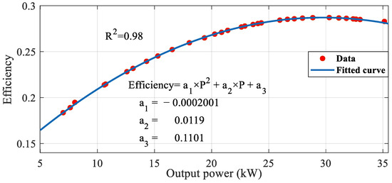
Figure 5.
Microturbine efficiency curve based on output power.
The equation of fuel cell costs is given in (12), and the cost of its fuel is given in Equation (13). The other costs including maintenance cost, start-up cost and emissions cost are formulated like those for microturbines [36].
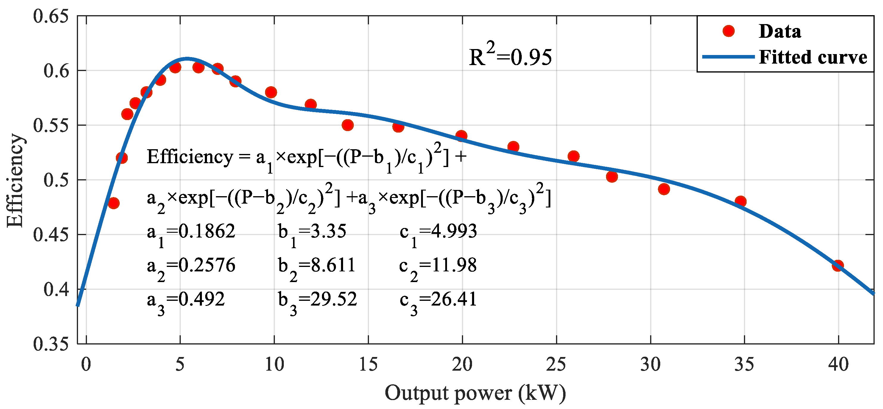
In Equation (13), PFC(t) is the fuel cell power at hour t, and ƞFC(t) is the fuel cell efficiency at hour (t). Figure 6 shows the fuel cell efficiency curve based on its output power. Using real data, the fuel cell estimated efficiency equation based on the output power is obtained through curve fitting. This figure also shows the value of the R2 criterion, which in this case is 0.95.
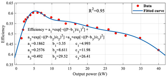
Figure 6.
Fuel cell efficiency curve based on output power.
Equation (14) describes diesel generator fuel consumption, which is modeled as a quadratic function.
where FDG is the value of fuel consumption in liters per hour, PDG(t) is the diesel generator power at hour t [24], and d, e and f are the fuel consumption coefficients of the diesel generator, which are equal to 0.4333, 0.2333 and 0.0074, respectively [21]. In order to convert the amount of fuel consumption into the cost of fuel consumption according to Equation (15), the price of one liter of diesel generator fuel (CF) can be multiplied by the value of fuel consumption.
The other costs including maintenance cost, start-up cost and emissions cost are formulated like those for microturbines. The diesel generator cost is modeled as Equation (16).
where FCDG is the diesel generator fuel cost, OCDG is the diesel generator maintenance cost, SCDG is the diesel generator start-up cost and ECDG is the environmental emission penalty cost.
The battery cost is obtained using the sum of the degradation cost and the maintenance cost [37].
where TCB is the battery cost, CDB is the degradation cost and PB(t) is the amount of charging or discharging power of the battery in hour t. For this parameter, a positive value means the amount of battery discharging, and a negative value means the amount of battery charging. NB is the number of batteries in the battery cells, CRB is the battery replacement cost, LB is the battery lifetime and COMB is the battery maintenance cost in one year. ƞB is the battery efficiency which is assumed to be the same in both charging and discharging modes.
Also, at any time, the amount of energy stored in the battery is calculated with Equation (19) [38].
where ES is the amount of energy stored in the battery, PcB is the amount of power in charging mode and PdB is the amount of power in discharging mode.
The battery parameters used in these equations are given in Table 1.

Table 1.
Battery technical and economical parameters [37].
In Table 1, SOCmin is the minimum battery state of charge (SOC), SOCmax is the maximum battery state of charge, Pmin is the maximum battery power in the discharging state, Pmax is the maximum battery power in the charging state, NB is the number of batteries in the battery cells, CRB is the battery replacement cost, LB is the battery lifetime and COMB is the battery maintenance cost in one year. Due to the constant costs of wind turbines and PV panels, they have been skipped in all three approaches.
In this work, the ACMG has the ability to transfer power with the main grid in all approaches. In the first approach, the DCMG is operated in islanded mode and does not have access to the main grid or to the ACMG.
In order to calculate the cost and revenue from power exchange with the main grid, Equations (20) and (21) can be used. The cost of purchased power from the main grid (CVNet) is formulated in Equation (20), and the revenue from selling power to the main grid (RVNet) is formulated in Equation (21).
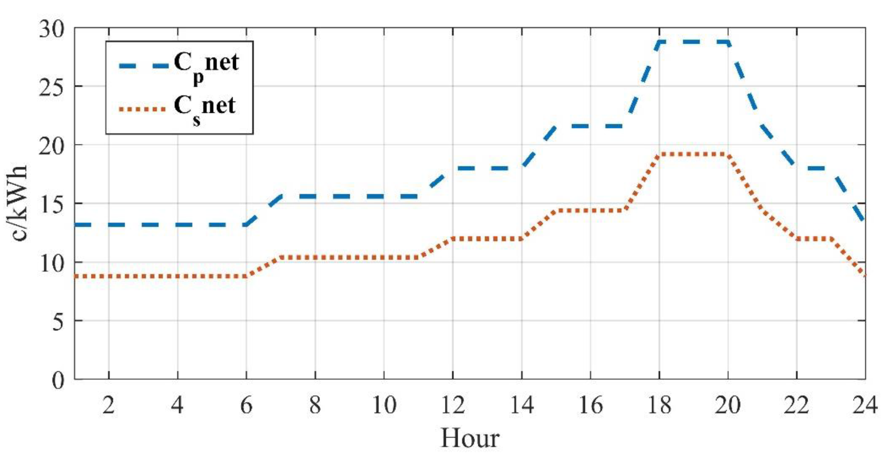
where PNet(t) is the power exchanged between the microgrid and the main grid at hour t, and Cp,Net(t) and Cs,Net(t) are the purchase price and sale price of 1 kW of power per cent at hour t, respectively.
In the second approach, in addition to the ability to exchange power with the main grid, it is possible for the ACMG to exchange power between two microgrids. The cost and revenue of exchanged power with the main grid in this approach are also the same as those for the first approach. The cost of purchasing and selling power for the ACMG to the DCMG and vice versa is as follows:
where RVAC,Inv is the revenue of the sale of ACMG power to the DCMG, which is equal to CVDC,Inv, which means the cost of purchasing DCMG power from the ACMG. RVDC,Inv is the revenue of selling DCMG power to the ACMG, and CVAC,Inv is the cost of purchasing ACMG power from the DCMG; these values are equal to each other. In this approach, from the DCMG point of view, the ACMG is the main grid, and the decision regarding the purchase or sale of power between the two microgrids is made by the DCMG.
In the third approach, the two microgrids are connected and data are transferred in such a way that two microgrids act as a single AC-DC microgrid. The transfer of power between these two microgrids is based on the overall revenue of the microgrids, and any cost is not considered for the power exchanged between the two microgrids. The cost and revenue of power exchange in this approach are related to power exchange with the main grid, whose equations are the same as the cost and revenue equations of the first approach.
3.1.3. Constraints
The obtained solutions should be applied to some constraints in optimization problems. The first constraint is the equality of generated and consumed power. In the first approach, there is a power equality condition for each of the microgrids. This condition for the ACMG is given as Equation (24), and that for the DCMG is given as Equation (25). In these equations, the amount of load connected to the microgrid must be equal to the amount of power generated by the resources.
where PL,ACMG and PL,DCMG are the consumed load of the ACMG and DCMG, respectively.
In the second approach, the power constraint for each microgrid is stated in Equations (26) and (27) for ACMG and DCMG, respectively.
where PInv(t) is the inverter (Inv) power that is placed between the two microgrids, PLI is the power loss in the inverter. It is assumed that half of these losses are provided by each of the two microgrids. It should be noted that the efficiency of the inverter is 95%.
In the third approach, the microgrid is operated as a single AC-DC microgrid, and both microgrids should supply the loads together. So, in this approach, there is a power equality constraint given as Equation (28).
Other constraints of the generation units including the maximum and minimum allowed generated power of each unit, the maximum and minimum amount of battery state of charge and the minimum time for the unit to start up or shut down are listed as follows:
In Equations (36) and (37), MUT and MDT are the minimum time in service and the minimum time out of service, respectively, and u is a binary variable related to whether the units are off or on. The index j represents the jth unit, and t is the desired time.
3.2. Decision Variables
In the first approach, the decision variables for the ACMG are microturbine power (PMT), diesel generator power (PDG) and power exchanged with the main grid (PNet). The decision variables for the DCMG are fuel cell power (PFC) and battery charge or discharge power (PB). In the second approach for the ACMG, the power exchanged through the inverter (PInv) will also be added as a decision variable. So, in the first and second approaches for the next 24 h, the ACMG has a 24 × 3 matrix, that is, 72 decision variables for optimization that should be solved simultaneously. For the DCMG in the first approach, we have a 24 × 2 matrix for optimization, that is, 48 decision variables. By adding the power exchanged through the inverter in the second approach, there is a 24 × 3 matrix with 72 decision variables to solve the optimization problem. In the third approach, connecting two microgrids with the presence of a common MCEMS will create a 24 × 6 matrix of decision variables. The state variables of each approach are shown in the following equations:
where An(DV1AC) and An(DV2AC) are the ACMG decision variables in the first approach and the ACMG decision variables in the second approach, respectively. An(DV1DC) and An(DV2DC) are the DCMG decision variables in the first approach and the DCMG decision variables in the second approach. An(DVAC-DC) represents the decision variables of the third approach.
3.3. Objective Functions
In this work, the objective function is cost minimization, and due to the existence of separate objectives for each microgrid in the first approach, the objective functions of the two microgrids are separate from each other. The objective functions of the DCMG and ACMG are given in Equations (42) and (43), respectively.
where CDCMG and CACMG are the costs of the DCMG and ACMG, respectively. Also, OFDC is the DCMG cost and OFAC is the ACMG cost. CVNet and RVNet are the cost of purchasing from the main grid and the revenue from the sale of power to the main grid, respectively.
The objective functions of the two microgrids in the second approach are still separate despite the connection between the two microgrids, and each microgrid seeks to minimize its own costs (not the total cost of the two microgrids). The objective functions of the two microgrids are expressed in the following equations:
In the third approach, considering that two microgrids are operated in the form of one AC-DC microgrid, the two microgrids set their decision variables with the same goal of minimizing the total costs of the two microgrids. The cost function of the third approach is expressed in Equation (46).
3.4. Proposed Method
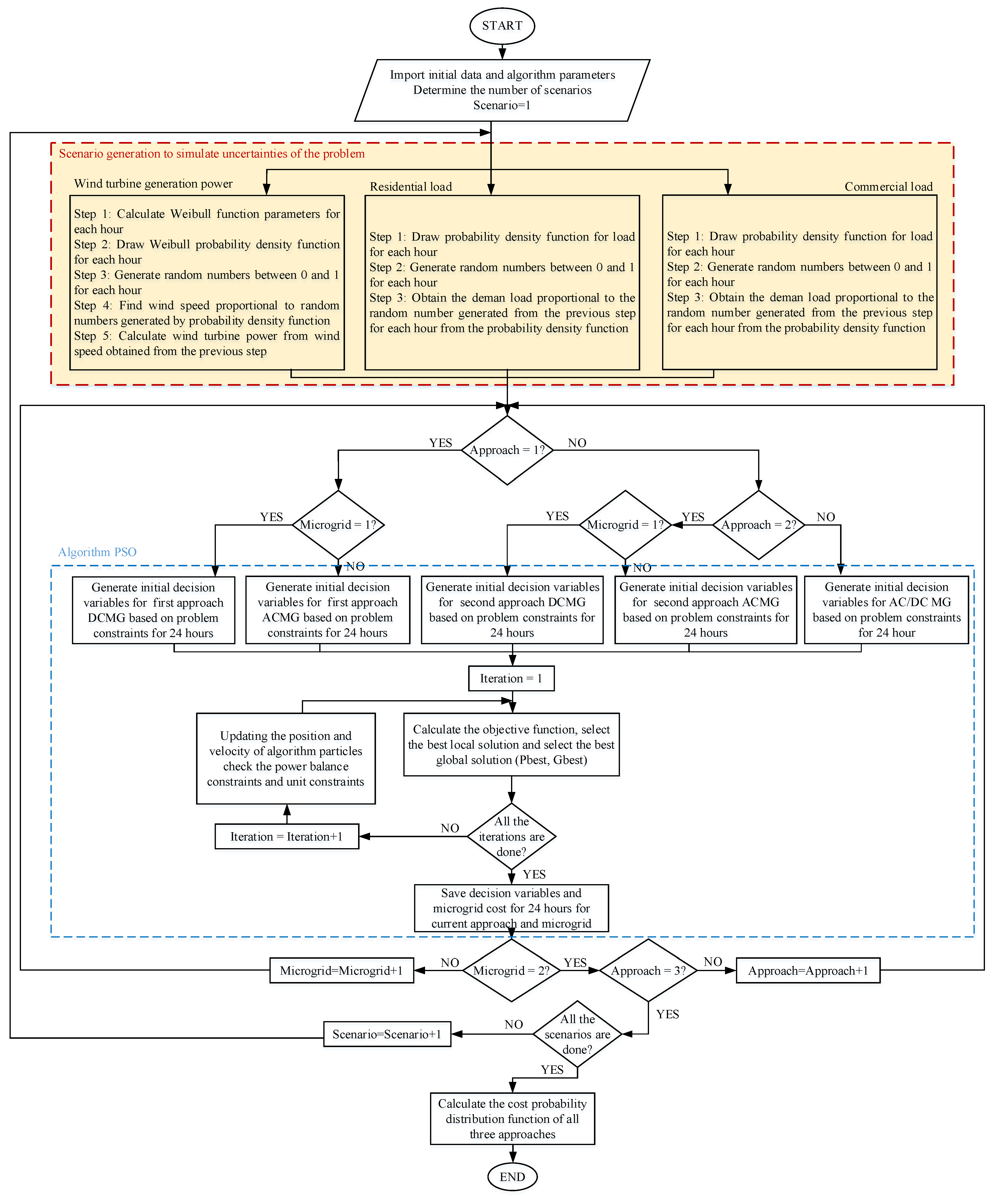
A flowchart illustrating the solving method for the proposed problem is shown in Figure 7. Initially, the algorithm takes in the required input data, including wind data, microgrid consumption loads, the number of simulation scenarios and the algorithm’s constants. During scenario generation, wind speed and load values for two microgrids are generated over a 24 h period using their respective distribution functions. These generated values serve as deterministic inputs for solving the next-day operation problem of the microgrids. The problem is then solved for each approach sequentially. The algorithm first examines the first approach, followed by the second and third approaches.
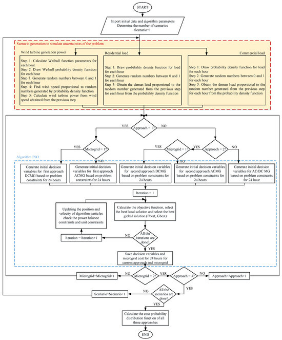
Figure 7.
Flowchart of the proposed method.
Within the algorithm, if the number of microgrids is set to one, the DCMG is evaluated. If the number of microgrids is set to two, the ACMG is also assessed. This means that operation management is first conducted for the DCMG. Then, based on the decision variables determined for the DCMG, the ACMG adjusts its own decision variables accordingly. In the first approach, since the two microgrids are not connected, their decisions are made independently of each other. However, in the second and third approaches, power management is first performed for the DCMG. The ACMG then determines its decision variables in response to those of the DCMG. Specifically, the ACMG must accommodate the DCMG’s power exchange requirements: supplying power when requested and receiving power when the DCMG needs to sell it.
In this paper, the PSO algorithm is used to solve the optimization problem [39]. The minimum value of objective functions for each approach and each microgrid will be determined by the values of the matrix of decision variables of each approach. In the PSO algorithm, particles have sub-particles for all the variables of the decision variable matrix. The inputs of the decision variable matrix are determined simultaneously and not hourly during the optimization process. For instance, in the DCMG in the first approach where there is a 48-input matrix, for particle number one of the PSO algorithm, a 48-input matrix corresponding to the decision variable matrix is generated. In each iteration, each input of the variable decision matrix changes at the same time as the other inputs, with the decision of the algorithm. This solves the algorithm to find the optimal solution by taking into account the future hours that affect the current hour decision. In this way, the simultaneous 24 h optimization required for the charging and discharging status of the batteries as well as the units being turned off or on is carried out in this algorithm.
At the end of each scenario, the algorithm checks that the calculations have been performed for the desired number of scenarios. The results of one scenario for wind data and load demand are presented to show the performance of the algorithm. Also, the cost probability distribution functions of the three approaches are simulated with the Monte Carlo method to demonstrate the effectiveness of the proposed method in the presence of wind and load demand uncertainties.
4. Simulation Results
4.1. Input Data
In this section, the initial data of generation units and loads are presented. The information related to the allowed power range for the operation of the generation units is presented in Table 2.
Table 2.
Permitted power range of the generation units [21].
The emission rate per kW of power generation units and the penalty factor for each of the pollutants is presented in Table 3.
Table 3.
Emission rate of generation power units and penalty factor for each of the pollutants [21].
The maintenance cost for each kW of power generation units is shown in Table 4.
Table 4.
Maintenance cost of power generation units [21].
The purchase and sale price of each kWh of energy in cents is shown in Figure 8.
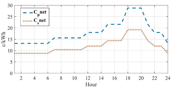
Figure 8.
Purchase and sale price of each kWh of energy in cents.
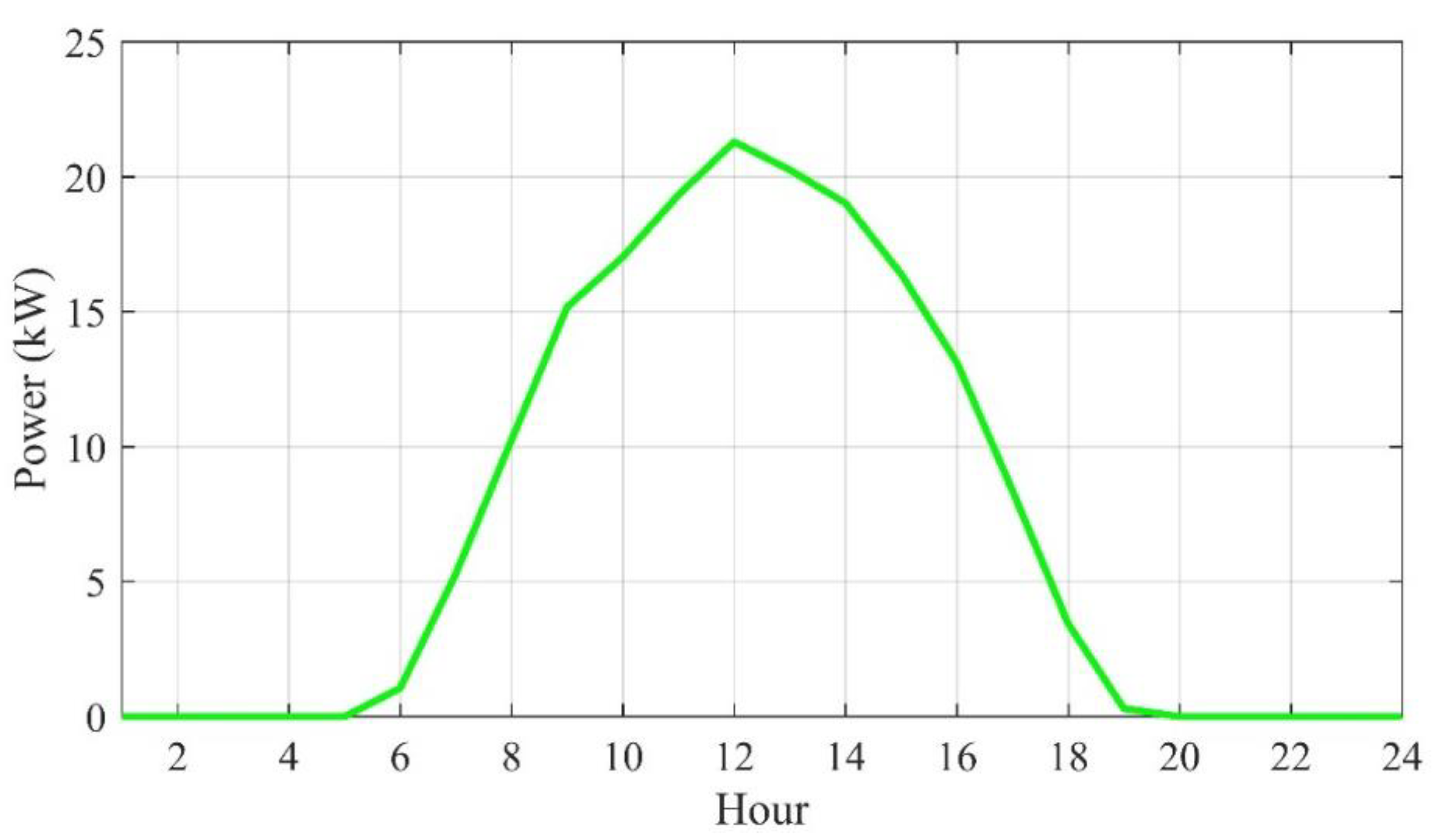
In the first step, the power generated by renewable units, such as wind turbine and PV units, as presented in Figure 9 and Figure 10, is subtracted from the load profile. So, the remaining load is the amount of power that should be supplied by programmable units and the main grid.
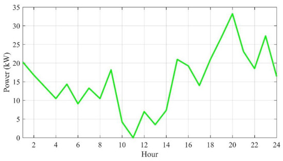
Figure 9.
Wind turbine generated power.

Figure 10.
Photovoltaic generated power.
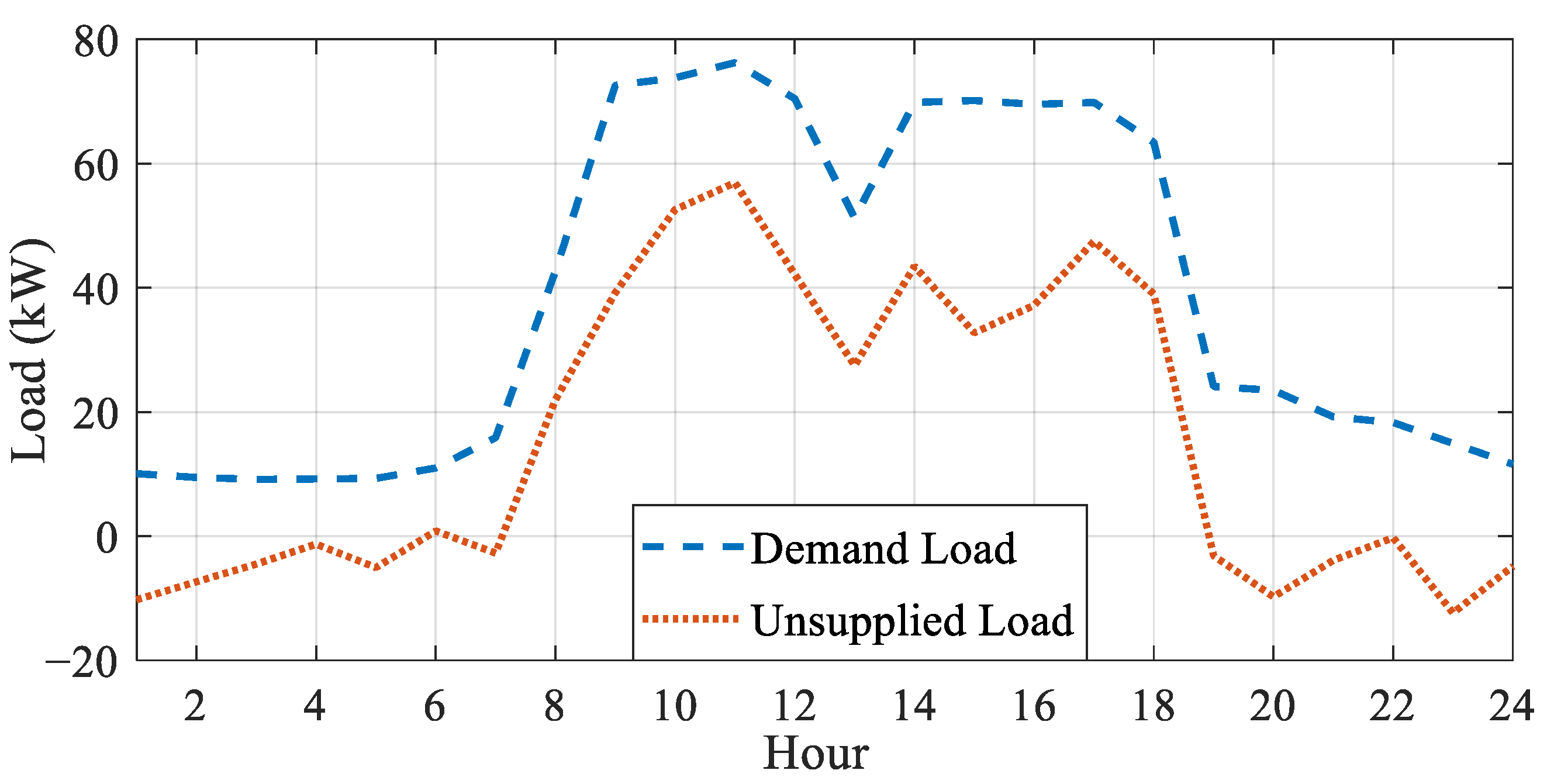
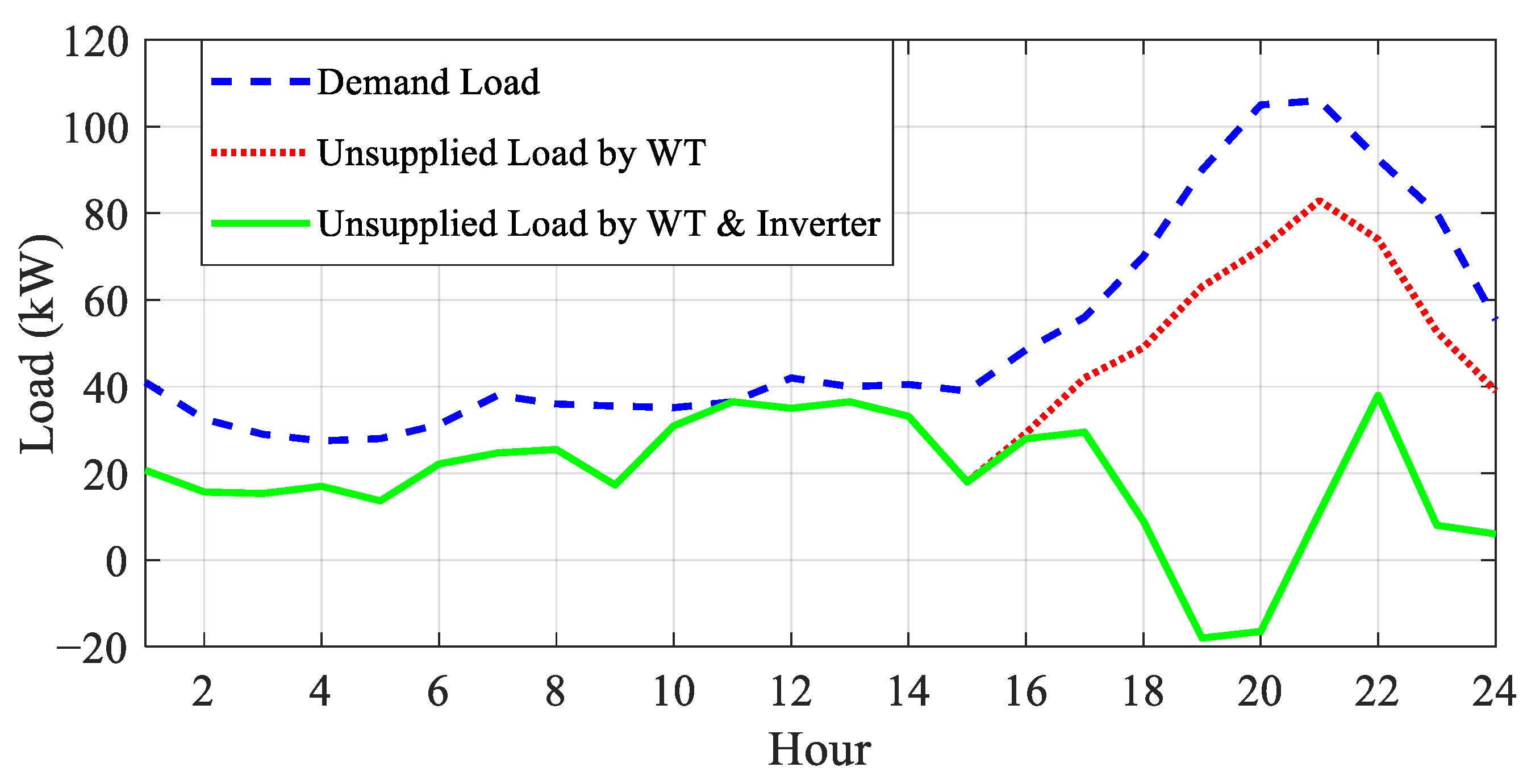
For the first approach, the unsupplied load of two microgrids is the amount of load obtained by subtracting the power of wind turbines and PV units in each microgrid from its initial load profile. Figure 11 shows the amount of load connected to the DCMG and the amount of load that is not supplied by WT and PV unit and must be supplied by programmable sources. In the second approach, first, the DCMG performs its programming for the day duration, and the amount of power transferred from the inverter is determined after the DCMG programming. So, in the second approach, the amount of load that should be supplied by the programmable units in the ACMG is obtained by subtracting the output power of the wind turbine in the ACMG and the power transferred from the DCMG from the initial load profile of the ACMG. In Figure 12, three curves are plotted. The dashed curve represents the total load connected to the microgrid. The dotted curve indicates the portion of the load that must be supplied from all sources except wind. The solid curve represents the load that must be supplied specifically by programmable sources (i.e., all sources except wind and power transferred from the microgrid).

Figure 11.
Demand load and unsupplied load profiles in the first approach for the DCMG.
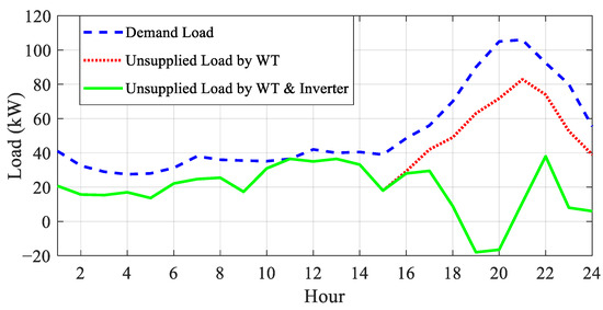
Figure 12.
Initial and unsupplied load profiles in the second approach for the ACMG.
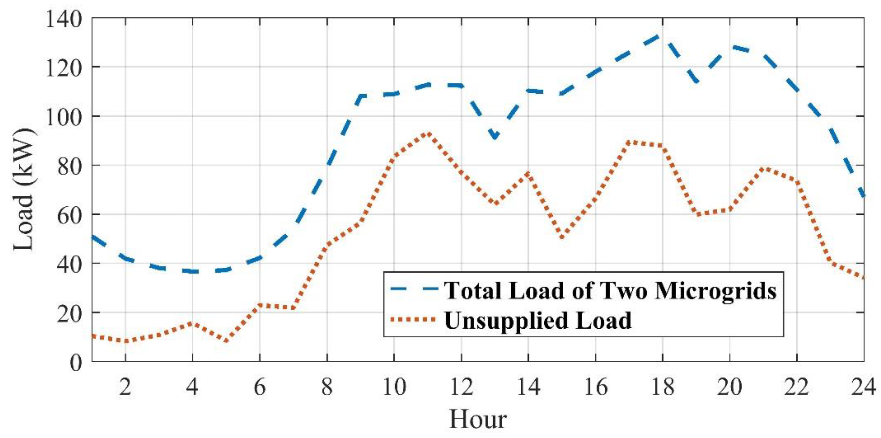
For the third approach, the initial AC-DC microgrid load profile is obtained from the total load profile of the ACMG and DCMG. The unsupplied load profile in this approach is obtained by subtracting the power of the two wind turbines in the two microgrids and the output power of the PV units. The initial and unsupplied load profile in the third approach is shown in Figure 13.
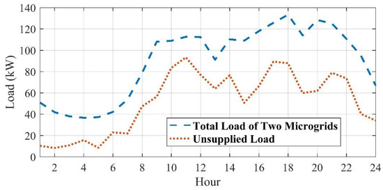
Figure 13.
Initial and unsupplied load profile in the third approach.
The output power of a PV unit is proportional to the amount of sun radiation. So, in the middle of the day when the amount of radiation is higher, the generated power of this unit is also higher. The load profile for the commercial load which is used in the middle of the day is similar to the output power of the PV unit. It can be seen that the output power of the PV unit will be consumed in the DCMG. On the other hand, the generated power of the wind turbine is relatively uniform throughout the day, and it is not limited to specific hours. In the first approach for the DCMG, at the end of the day, due to the sharp reduction in demand load, the excess power generated by this unit will remain unused. In the above-mentioned load profiles, the negative values of the load profile mean excess power generation. As can be seen for the first approach, in the hours between 1:00 to 7:00 and 19:00 to 24:00, the demand power profile for the DCMG becomes negative after applying the power of the wind turbine and PV unit. Since two microgrids are not connected in this approach, the excess power cannot be transferred to the ACMG or main grid.
With the possibility of power exchange in the second approach, the excess power of the DCMG can be sold to the ACMG as revenue for this microgrid. Figure 12 shows that in the second approach for peak hours of the ACMG, the demand load profile will decrease significantly after applying the wind turbine power as well as the power transmitted through the inverter. Since DCMG power is a cheaper choice for the ACMG than the power from the main grid, power exchange in peak hours for the ACMG will reduce costs. In the third approach, with the total demand load of two microgrids, the load profile will be more uniform. In this approach, the load profile will be provided with the presence of all the units. So, the adjustment points of the decision variables of the units will be determined according to the performance of the two microgrid units.
4.2. Results of Three Proposed Approaches
In the first approach, the two microgrids are not connected, and the battery is only used to set the optimal decision points of the fuel cell. According to the demand power of the DCMG, the battery is charged or discharged every hour so that the fuel cell works at its best efficiency point for 24 h. The battery is charged in the early hours of the operation time and discharged in the middle of the day due to the increasing DCMG power demand. Also, in this approach, the battery is charged from 19:00 until the end of the day, due to the sharp reduction in power consumption in the DCMG and the presence of excess power over consumption. Figure 14 shows the battery state of charge in the first approach.
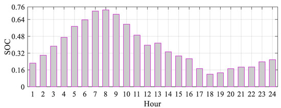
Figure 14.
Battery state of charge in the first approach.
Due to the two microgrids not being connected in the first approach, the fuel cell, which is a unit with good efficiency, has no power generation from 19:00 onwards despite the price of electricity increasing. This issue shows the loss of the opportunity for fuel cell participation in ACMG power supply as well as selling power to the main grid. Due to the operation of the DCMG in the islanded mode in this approach and not connecting with the main grid, the price of power is not involved in determining the decision variables of this microgrid. In the ACMG, the diesel generator will not generate power because of the high cost of emissions and lower efficiency compared to the other units. The microturbine, which has good efficiency, will be able to generate power when the generation cost of this unit is lower than the cost of the main grid. Figure 15 and Figure 16 present the optimal operation points or the amount of power generated by units in the first approach for the DCMG and the ACMG, respectively.
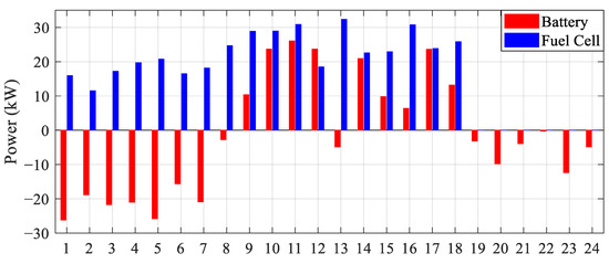
Figure 15.
Optimal operation points of the DCMG units in the first approach.

Figure 16.
Optimal operation points of the ACMG units in the first approach.
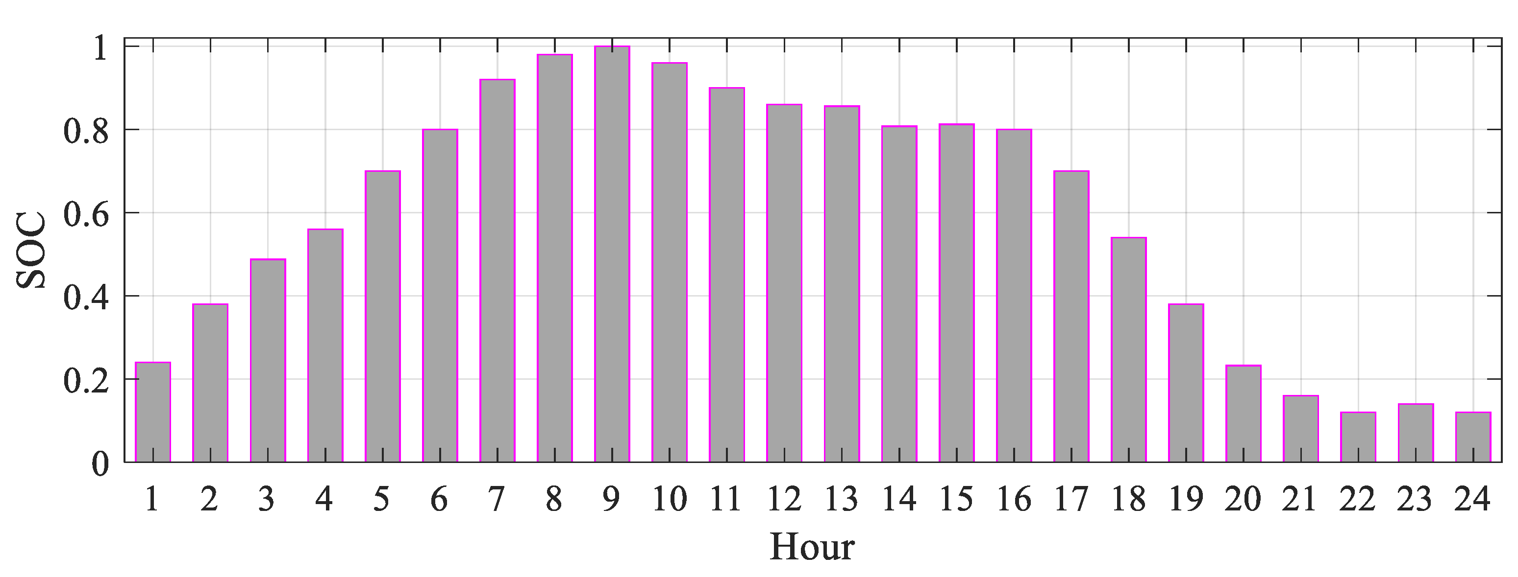
In the second approach, due to the possibility of power exchange for the DCMG and the low price of energy in the early hours of the day, the battery is charged during these hours. In this approach, most of the battery discharging process is done during the hours when the price of energy is higher, unlike the first approach which was in the middle of the day because of the demand power of the DCMG. The battery state of charge in the second approach is shown in Figure 17. It can be seen from Figure 17 that, unlike the first approach, the battery state of charge reaches its minimum value (30 kW) in the last hour of the day. This shows that the battery has used all its possible power storage to sell and supply the load and adjust the optimal decision points of the fuel cell, which will increase the battery’s contribution to minimize the costs.
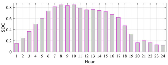
Figure 17.
Battery state of charge in the second approach.
Considering the high efficiency of the fuel cell unit and providing the possibility of power transfer of this unit for sale to the other microgrid, the generated power of this unit has increased significantly in the second approach compared to the first approach. The DCMG receives power through the inverter during the required hours, and on the other hand, due to the high price of energy at night hours, it sells power to the ACMG through the inverter. The optimal operation points of the ACMG units in the second approach are shown in Figure 18. The negative amount of inverter power in Figure 18 means the transfer of power from the DCMG to the ACMG.
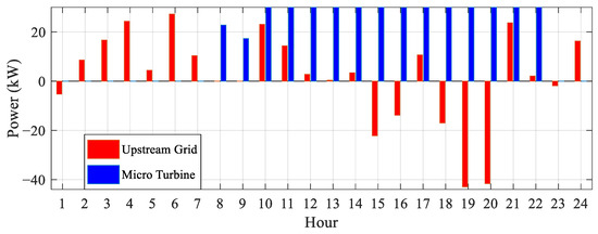
Figure 18.
Optimal operation points of the ACMG units in the second approach.
In the second approach, like the first approach, the microturbine generates power when the cost of generating power of this unit is less than the main grid or it is required to generate power. Due to the increasing efficiency of the microturbine unit with an increase in its power generation, it works at its maximum allowable power when the cost of generating power of this unit is less than the price of sale to the main grid. The optimal operation points of the DCMG units in the second approach are shown in Figure 19.

Figure 19.
Optimal operation points of the DCMG units in the second approach.
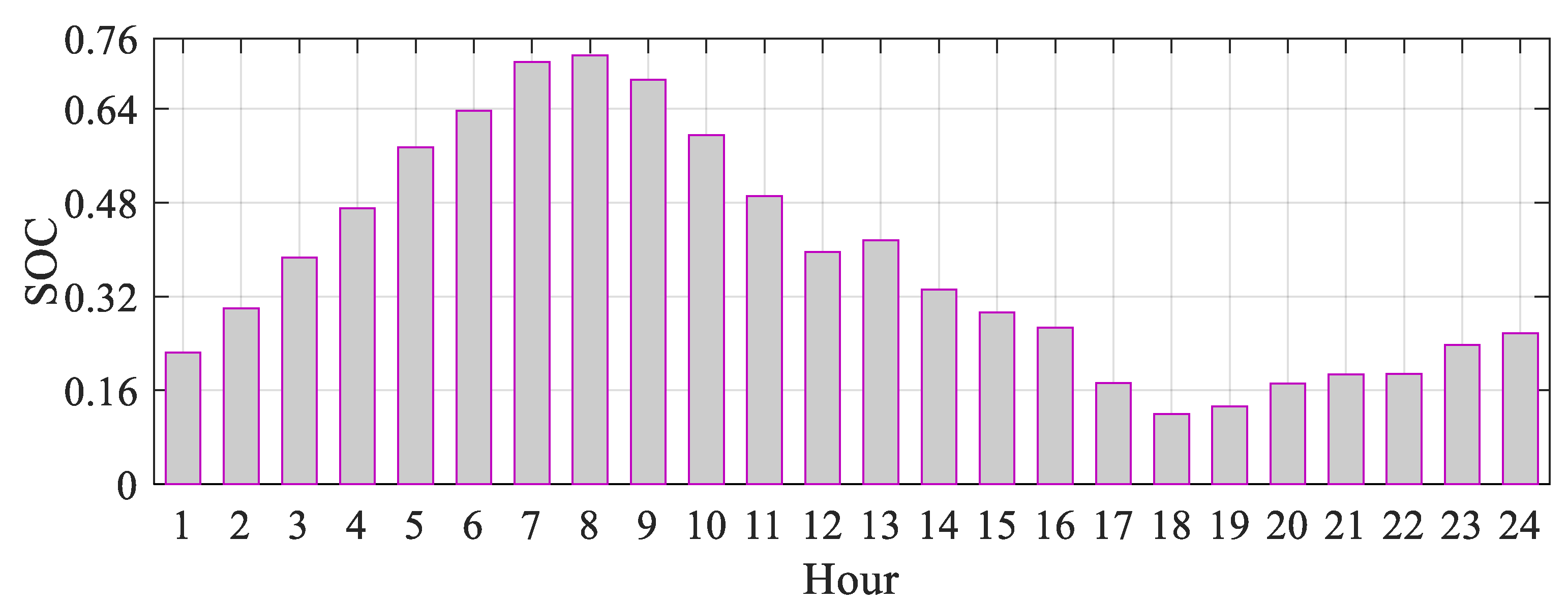
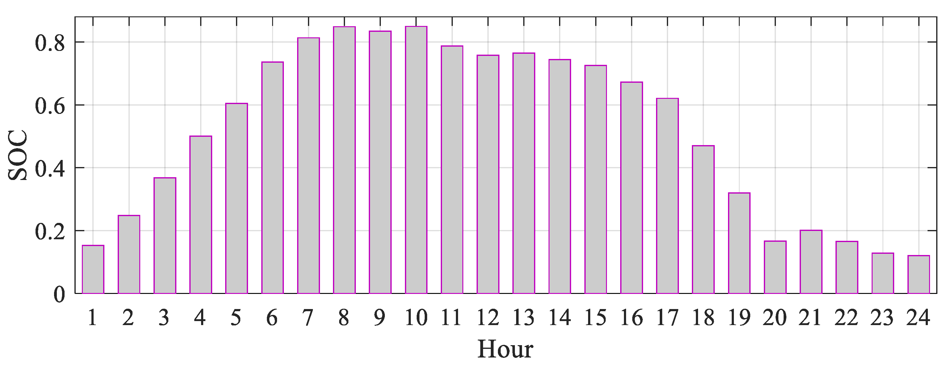
In the third approach, due to the connection of two microgrids and the existence of a single central management system, the units in the microgrid will operate to minimize the total cost of the two microgrids. The coordination of programmable units in this approach reduces the total cost of two microgrids. In this approach, the battery is charged during the hours when the energy price is lower and discharged during the hours when the price is higher. Also, like other programmable units, the battery will help to optimally set the decision points of two microgrid units. The battery state of charge in the third approach is shown in Figure 20.
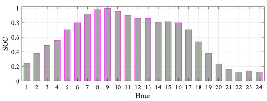
Figure 20.
Battery state of charge in the third approach.
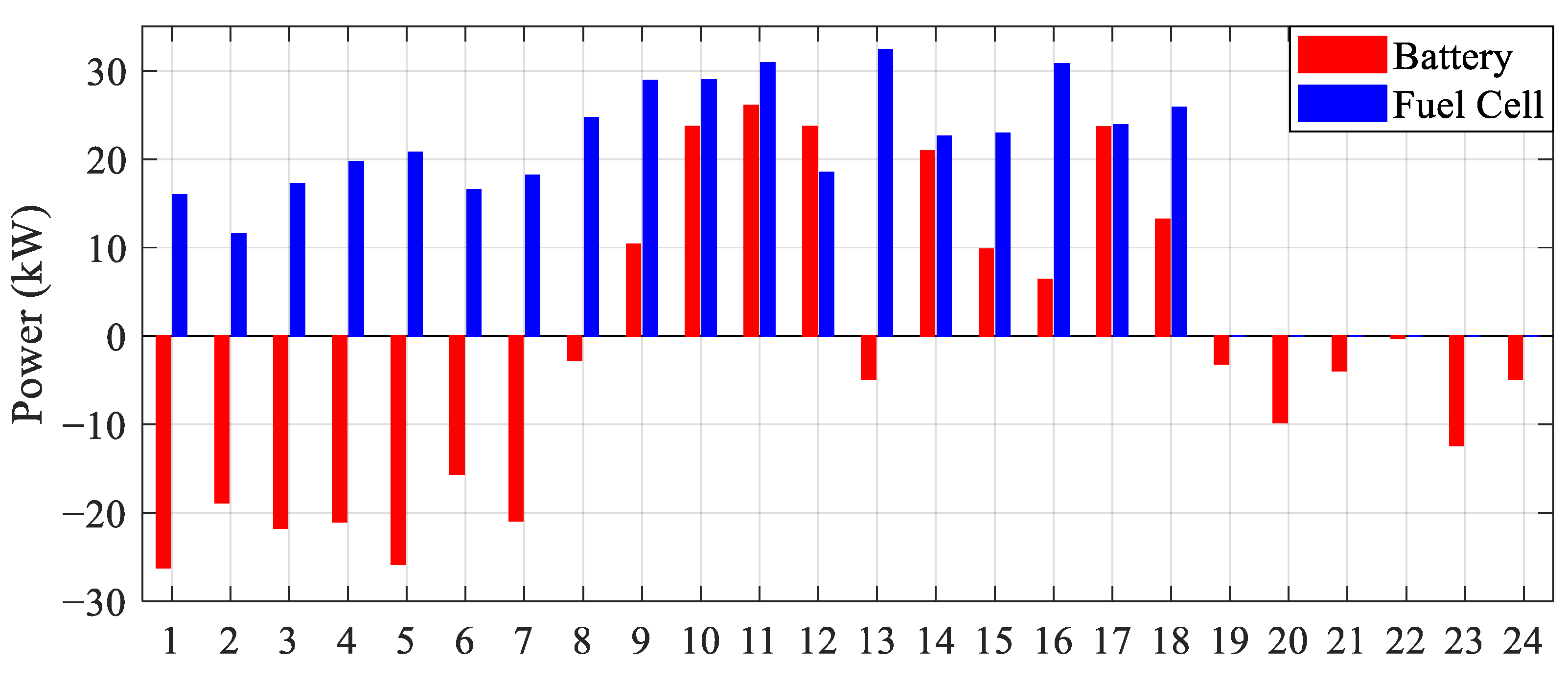
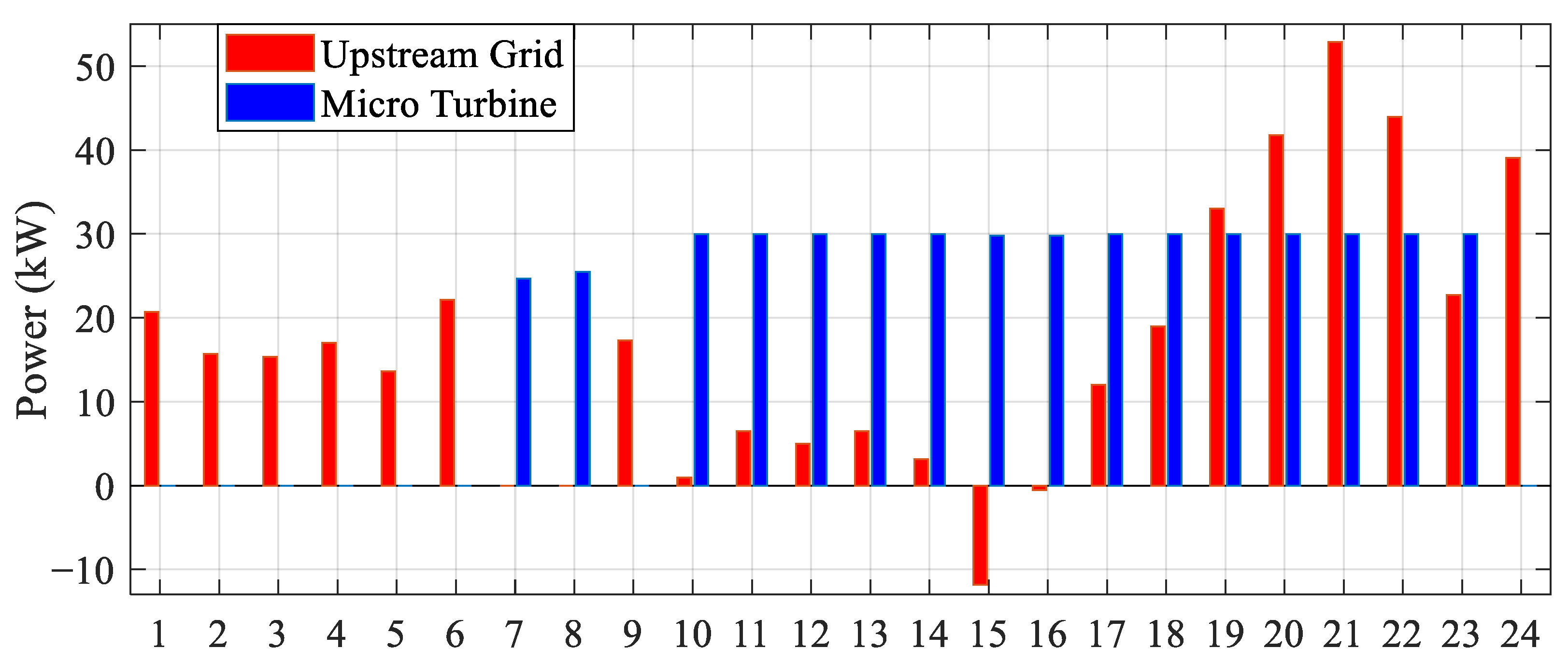
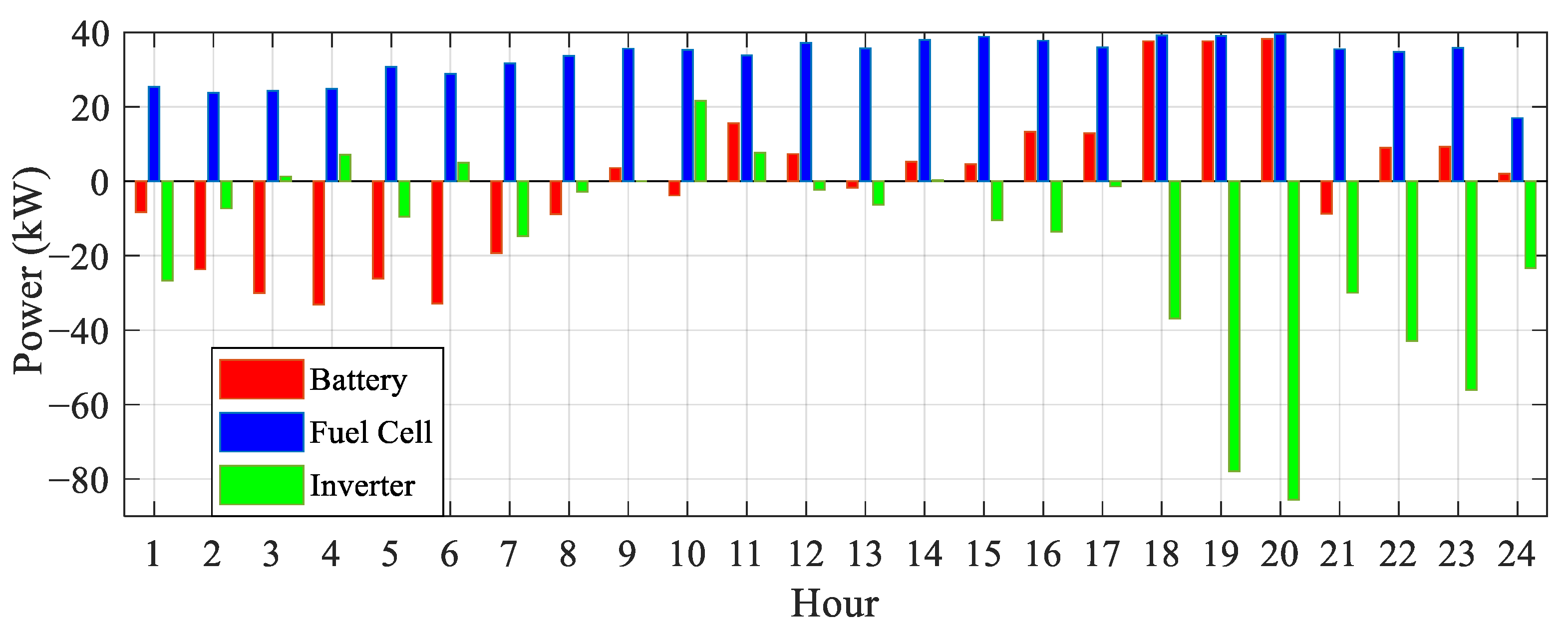
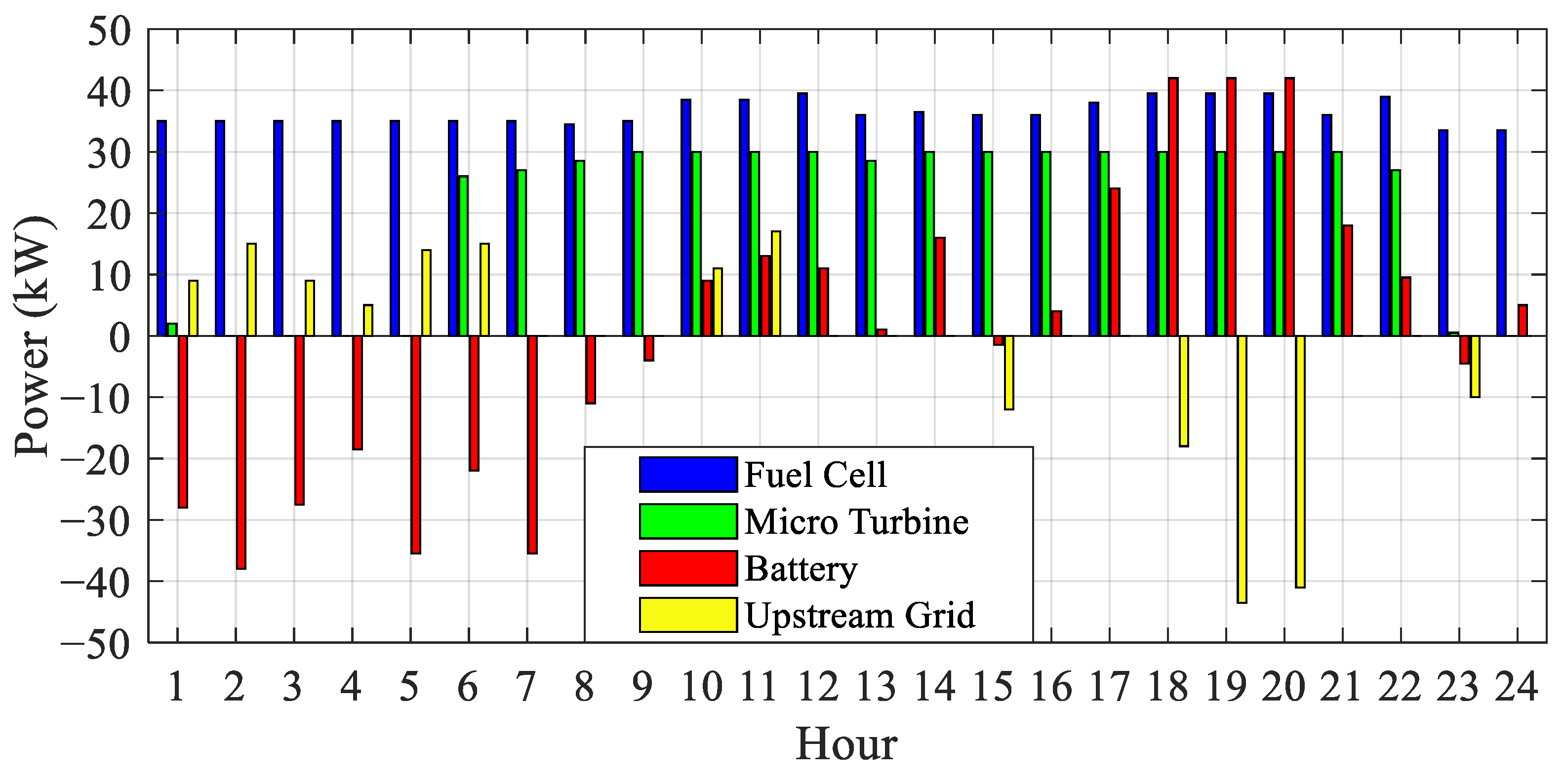
The optimal operation points of microgrid units in the third approach are shown in Figure 21. In this approach, in the early hours, due to the lower energy price, power is received from the main grid, and due to the low power consumption of loads during these hours, some of the power injected into the network will be used to charge the battery. In hours when the energy price increases and the amount of power generated by other sources increases, and it is also possible to use the energy stored in the battery, the excess power consumed by the loads is sold to the main grid. Negative power values for the main grid mean the sale of power to the main grid.
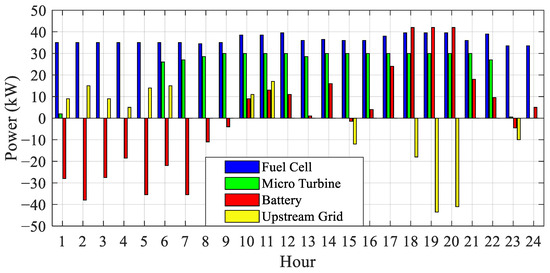
Figure 21.
Optimal operation points of microgrid units in the third approach.
The summary of the above-mentioned simulation results can be summarized as follows:
- Operating microgrids in islanded mode reduces the potential for distributed generation to fully meet the load demand.
- The battery’s performance differs between the islanded mode and grid-connected mode. In the islanded mode, the battery primarily functions as a regulator, maintaining the optimal operating point of programmable units.
- The presence of an MCEMS in microgrid connections enables power to be drawn from the main grid during early hours when energy prices are lower.
- During periods of higher energy prices and increased power generation from other sources, excess power consumed by the loads is sold back to the main grid.
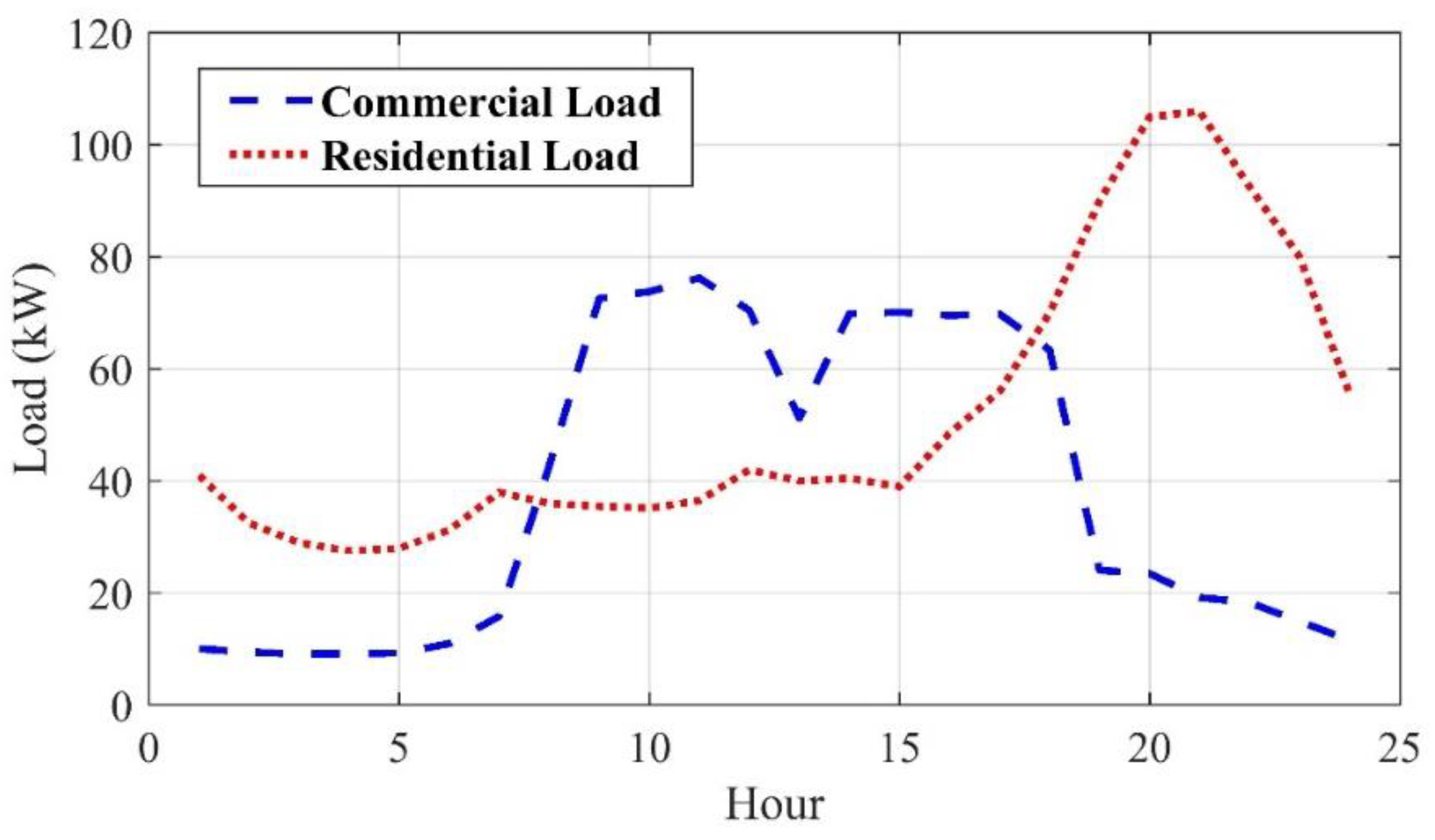
In order to investigate the costs of three approaches in the presence of load and wind uncertainties, 30 different scenarios of wind and load are generated, and the performance of microgrids under these data is evaluated as an input with the Monte Carlo simulation method. Figure 22 shows the commercial and residential load curves used in the DCMG and ACMG. The standard deviation for loads in this work is considered 4% for each hour [37].
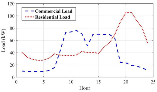
Figure 22.
Commercial load curve for the DCMG and residential load curve for the ACMG.
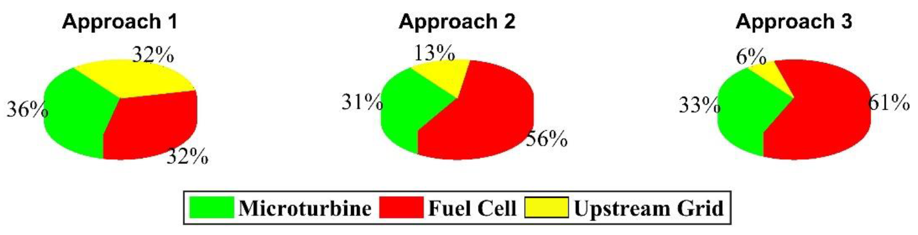
In Figure 23, the percentage of units participating in the generation of required power is presented. The percentage of power generation by diesel generator, microturbine and fuel cell units and the power purchased from the main grid will be 0, 31, 56 and 13 percent, respectively, and for the third approach, they will be 0, 33, 61 and 6 percent, respectively. This indicates that the participation of the fuel cell unit, which is an economic unit, has increased, and the power purchased from the main grid has decreased. This reduction in purchased power is mainly due to the exchange of power between two microgrids, which benefits both microgrids.

Figure 23.
Percentage of units participating in the generation of required power.
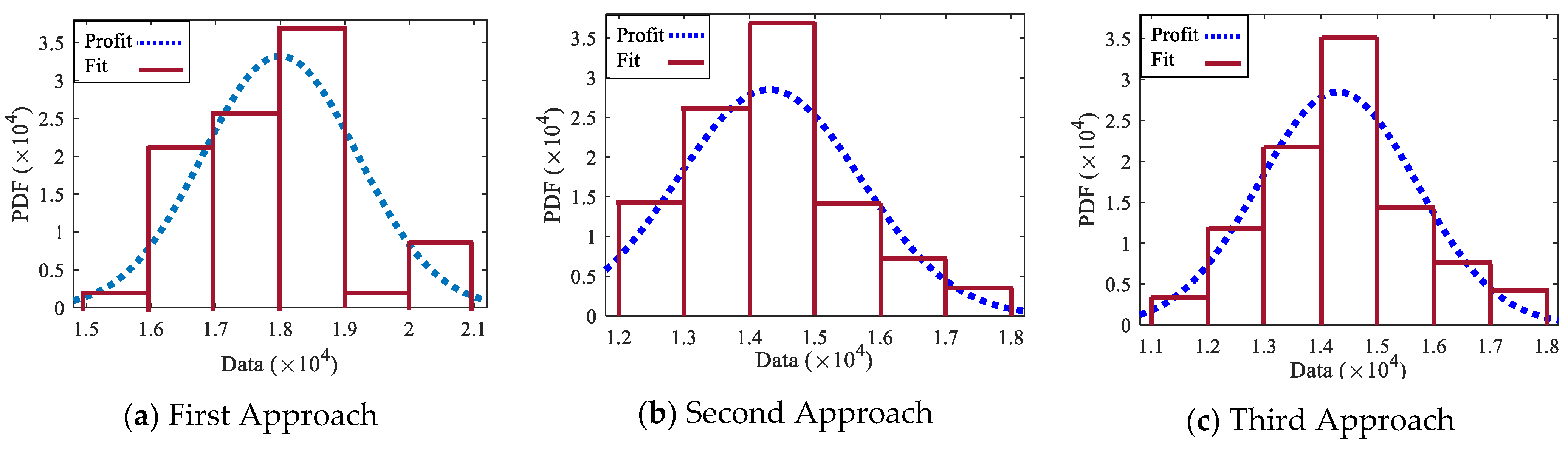
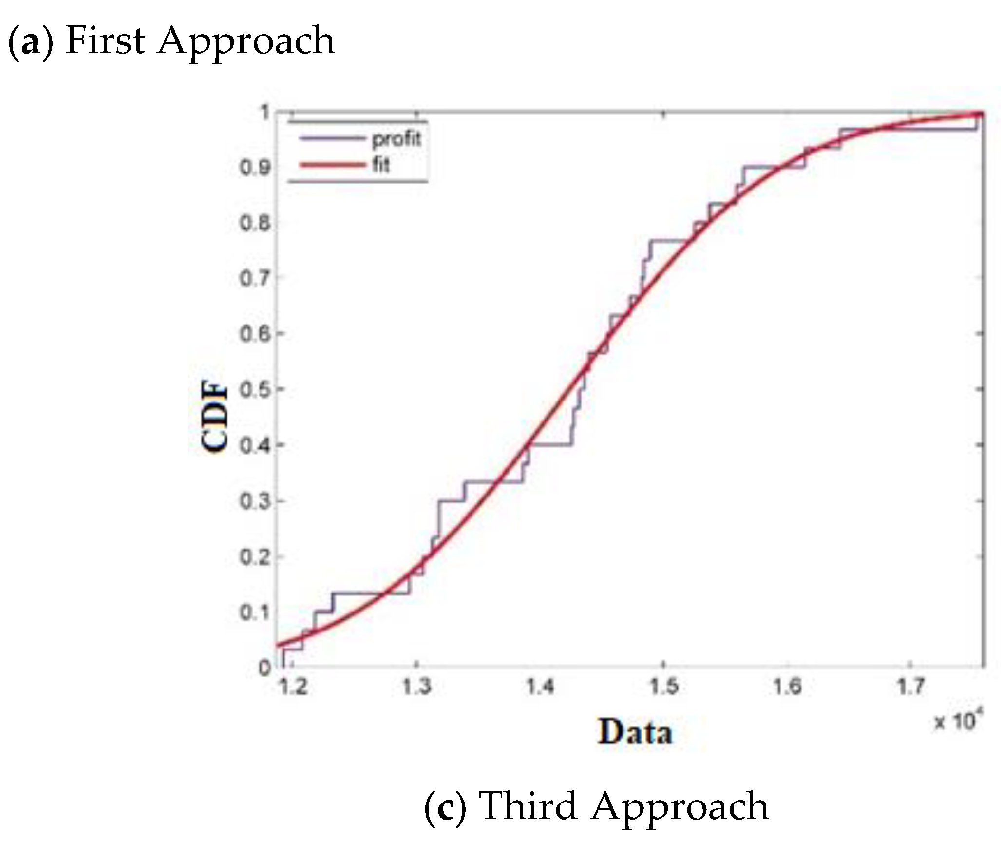
The probabilistic simulation of the uncertainties for the three approaches is performed, and the probability distribution functions and the cumulative distribution functions are shown in Figure 24 and Figure 25. Figure 24 shows the probability distribution function for the three approaches. Also, Figure 25 shows the cumulative distribution function for all three approaches. It can be concluded from these figures that connecting microgrids in the second and third approaches has a significant impact on minimizing the total cost of microgrids.
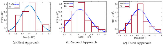
Figure 24.
Cost probability distribution function (PDF) in the (a) first, (b) second and (c) third approaches.
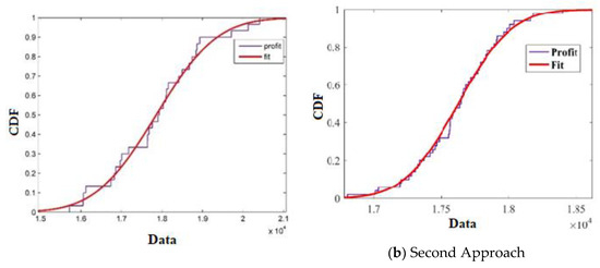

Figure 25.
Cost cumulative probability distribution function (CDF) in the (a) first, (b) second and (c) third approaches.
The cost of the three approaches simulated by a scenario of wind speed and load demand is shown in Table 5.
Table 5.
Cost of the three approaches for a selected scenario.
The total cost of the two microgrids in the third approach has the lowest value according to its objective function which is to minimize the total costs. In the second approach, considering that every microgrid prioritizes minimizing its own costs, the DCMG cost is lower than that for the third approach. This means that in the third approach, despite the reduction in the total costs of the two microgrids, the cost of one of the microgrids will be higher. The third approach will make sense when two microgrids are operated to achieve a common goal and each of them prioritizes minimizing the profit of the two microgrids. In the first approach, the costs of the two microgrids will be higher than those of other approaches because the two microgrids are not connected.
Simulations in the presence of wind and load demand uncertainties show that the connection of AC and DC microgrids leads to cost reduction considering uncertainties. Another difference between the second and third approaches is in the dimensions of the system variable matrix of the two approaches. Reducing the dimensions of the system matrix in the second approach increases the speed of solving the algorithm for the second approach compared to the third approach.
Suggestions that can be considered as future work for this research include:
- Applying multi-objective optimization methods in the operation of an AC/DC microgrid.
- Considering the presence of electric vehicles in the DC section.
- Evaluating the operation of an AC/DC microgrid while accounting for power losses.
- Analyzing unbalanced microgrids.
- Incorporating stochasticity in other parameters, such as energy costs or the state of charge (SOC) of the battery.
5. Conclusions
In this paper, first, two microgrids are examined in a separate mode, and then two approaches are proposed for the operation of two AC and DC microgrids when connected. Connections between the DCMG, ACMG and main grid are considered in different modes. In the second operation approach, despite the connection of the two microgrids, each microgrid has its own independent MCEMS. The results of this approach are a reduction in the dimensions of the matrix of decision variables and an increase in the speed of problem-solving considering separate MCEMSs and prioritizing the individual costs of each owner instead of the total cost of microgrids. In the third approach, using a common MCEMS for the two microgrids, a single AC-DC microgrid is created, which aims to minimize the total cost of the two microgrids. The results demonstrate that the third approach has succeeded in minimizing the total cost of the two microgrids. By comparing the costs associated with the first and third approaches, it is evident that the cost reduction in the DCMG is 67.9 percent, in the ACMG is 14.2 percent, and overall is 24.4 percent. This cost reduction can be attributed to the implementation of the MCEMS, as it reduces reliance on main grid power and instead utilizes alternative sources such as the fuel cell. According to the results of the first and third approaches, the participation of the fuel cell in supplying microgrid loads has increased by 29 percent, while the participation of the main grid has decreased by 26 percent. The connections of the two microgrids in different approaches have been evaluated with a scenario, and the results demonstrate that the proposed approaches are economical for both microgrids. Also, different wind and load scenarios are generated to consider the uncertainties in the problem, and the results are presented in the form of probability distribution functions for the three approaches.
Author Contributions
Conceptualization, H.Z.-M.; methodology, H.Z.-M. and R.S.; software, H.Z.-M. and R.S.; validation, F.N.; formal analysis, H.Z.-M., R.S. and F.N.; investigation, H.Z.-M. and F.N.; resources, F.N.; data curation, H.Z.-M. and R.S.; writing—original draft preparation, H.Z.-M. and R.S.; writing—review and editing, F.N.; visualization, H.Z.-M. and R.S.; supervision, F.N.; project administration, H.Z.-M. and F.N.; funding acquisition, F.N. All authors have read and agreed to the published version of the manuscript.
Funding
This research received no external funding.
Data Availability Statement
The data that support the findings of this study are available from the corresponding author upon reasonable request.
Acknowledgments
For the purpose of open access, the author has applied a Creative Commons Attribution (CC BY) license to any Author Accepted Manuscript version arising from this submission.
Conflicts of Interest
The authors declare that there are no conflicts of interest.
Abbreviation
| ACMG | AC Microgrid |
| DCMG | DC Microgrid |
| DG | Diesel Generator |
| FC | Fuel Cell |
| Inv | Inverter |
| MCEMS | Microgrid Central Energy Management System |
| MT | Microturbine |
| PSO | Particle Swarm Optimization |
| PV | Photovoltaic |
| SOC | State of Charge |
| WT | Wind Turbine |
References
- Wang, C.; Zhang, Z.; Abedinia, O.; Farkoush, S.G. Modeling and analysis of a microgrid considering the uncertainty in renewable energy resources, energy storage systems and demand management in electrical retail market. J. Energy Storage 2021, 33, 102111. [Google Scholar] [CrossRef]
- Niknam, T.; Zeinoddini-Meymand, H.; Mojarrad, H.D. A novel Multi-objective Fuzzy Adaptive Chaotic PSO algorithm for Optimal Operation Management of distribution network with regard to fuel cell power plants. Eur. Trans. Electr. Power 2011, 21, 1954–1983. [Google Scholar] [CrossRef]
- Safipour, R.; Oukati Sadegh, M. Optimal Planning of Energy Storage Systems in Microgrids for Improvement of Operation Indices. Int. J. Renew. Energy Res. 2018, 18, 1483–1498. [Google Scholar] [CrossRef]
- Prasad, T.N.; Devakirubakaran, S.; Mithubalaji, S.; Srinivasan, S.; Karthikeyan, B.; Palanisamy, R.; Bajaj, M.; Zawbaa, H.M.; Kamel, S. Power management in hybrid ANFIS PID based AC–DC microgrids with EHO based cost optimized droop control strategy. Energy Rep. 2022, 8, 15081–15094. [Google Scholar] [CrossRef]
- Modarresi, J. Coalitional game theory approach for multi-microgrid energy systems considering service charge and power losses. Sustain. Energy Grids Netw. 2022, 31, 100720. [Google Scholar] [CrossRef]
- García-Ceballos, S.P.-L.C.; Mora-Flórez Londono, S.P.J.; Ceballos, C.G.; Flórez, J.M. Stability analysis framework for isolated microgrids with energy resources integrated using voltage source converters. Results Eng. 2023, 19, 101252. [Google Scholar] [CrossRef]
- Raju, D.K.; Kumar, R.S.; Raghav, L.P.; Singh, A.R. Enhancement of loadability and voltage stability in grid-connected microgrid network. J. Clean. Prod. 2022, 374, 101252. [Google Scholar] [CrossRef]
- Muyeen, S.M.; Gholami, M.; Mousavi, S.A. Development of new reliability metrics for microgrids: Integrating renewable energy sources and battery energy storage system. Energy Rep. 2023, 10, 2251–2259. [Google Scholar]
- Szilagyi, E.; Petreus, D.; Paulescu, M.; Patarau, T.; Hategan, S.M.; Sarbu, N.A. Cost-effective energy management of an islanded microgrid. Energy Rep. 2023, 10, 4516–4537. [Google Scholar] [CrossRef]
- Kassab, F.A.; Celik, B.; Locment, F.; Sechilariu, M.; Liaquat, S.; Hansen, T.M. Optimal sizing and energy management of a microgrid: A joint MILP approach for minimization of energy cost and carbon emission. Renew. Energy 2024, 224, 120186. [Google Scholar] [CrossRef]
- Caminiti, C.M.; Ragaini, E.; Barbieri, J.; Dimovski, A.; Merlo, M. Limited-Size BESS for Mitigating the Impact of RES Volatility in Grid-Tied Microgrids in Developing Countries: Focus on Lacor Hospital. In Proceedings of the 2024 IEEE PES/IAS PowerAfrica, Johannesburg, South Africa, 7–11 October 2024. [Google Scholar]
- Khajeh, A.; Modarress, H.; Zeinoddini-Meymand, H. Application of modified particle swarm optimization as an efficient variable selection strategy in QSAR/QSPR studies. J. Chemom. 2012, 26, 598–603. [Google Scholar]
- Nejabatkhah, F.; Li, Y.W. Overview of Power Management Strategies of Hybrid AC/DC Microgrid. IEEE Trans. Power Electron. 2015, 30, 7072–7089. [Google Scholar]
- Gupta, A.; Doolla, S.; Chatterjee, K. Hybrid AC–DC Microgrid: Systematic Evaluation of Control Strategies. IEEE Trans. Smart Grid 2018, 9, 3830–3843. [Google Scholar]
- Sohrabi-Tabar, V.; Jirdehi, M.A.; Hemmati, R. Energy management in microgrid based on the multi objective stochastic programming incorporating portable renewable energy resource as demand response option. Energy 2017, 118, 827–839. [Google Scholar] [CrossRef]
- Firouzi, B.; Zeinoddini-Meymand, H.; Niknam, T.; Mojarrad, H.D. A novel multi-objective Chaotic Crazy PSO algorithm for optimal operation management of distribution network with regard to fuel cell power plants. Int. J. Innov. Comput. Inf. Control 2011, 7, 6395–6409. [Google Scholar]
- Baziar, A.; Kavousi-Fard, A. Considering uncertainty in the optimal energy management of renewable micro-grids including storage devices. Renew. Energy 2013, 59, 158–166. [Google Scholar]
- Siahkali, H.; Vakilian, M. Stochastic unit commitment of wind farms integrated in power system. Electr. Power Syst. Res. 2010, 80, 1006–1017. [Google Scholar]
- Kumar, R.P.; Karthikeyan, G. A multi-objective optimization solution for distributed generation energy management in microgrids with hybrid energy sources and battery storage system. J. Energy Storage 2024, 75, 109702. [Google Scholar]
- Babu, V.V.; Roselyn, J.P.; Sundaravadivel, P. Multi-objective genetic algorithm based energy management system considering optimal utilization of grid and degradation of battery storage in microgrid. Energy Rep. 2023, 9, 5992–6005. [Google Scholar]
- Moradi, H.; Esfahanian, M.; Abtahi, A.; Zilouchian, A. Optimization and energy management of a standalone hybrid microgrid in the presence of battery storage system. Energy 2018, 147, 226–238. [Google Scholar]
- Li, Z.; Xie, X.; Cheng, Z.; Zhi, C.; Si, J. A novel two-stage energy management of hybrid AC/DC microgrid considering frequency security constraints. Electr. Power Energy Syst. 2023, 146, 108768. [Google Scholar] [CrossRef]
- Yuan, G.; Wang, H.; Khazaei, E.; Khan, B. Collaborative advanced machine learning techniques in optimal energy management of hybrid AC/DC IoT-based microgrids. Ad Hoc Netw. 2021, 122, 102657. [Google Scholar]
- Billah, M.; Yousif, M.; Numan, M.; Salam, I.U.; Kazmi, S.A.A.; Alghamdi, T.A.H. Decentralized Smart Energy Management in Hybrid Microgrids: Evaluating Operational Modes, Resources Optimization, and Environmental Impacts. IEEE Access 2023, 11, 143530–143548. [Google Scholar]
- Bacha, B.; Ghodbane, H.; Dahmani, H.; Betka, A.; Toumi, A.; Chouder, A. Optimal sizing of a hybrid microgrid system using solar, wind, diesel, and battery energy storage to alleviate energy poverty in a rural area of Biskra, Algeria. J. Energy Storage 2024, 84, 110651. [Google Scholar]
- Yang, F.; Ye, L.; Muyeen, S.M.; Li, D.; Lin, S.; Fang, C. Power management for hybrid AC/DC microgrid with multi-mode subgrid based on incremental costs. Electr. Power Energy Syst. 2022, 138, 107887. [Google Scholar]
- Cai, Y.; Lu, Z.; Pan, Y.; He, L.; Guo, X.; Zhang, J. Optimal scheduling of a hybrid AC/DC multi-energy microgrid considering uncertainties and Stackelberg game-based integrated demand response. Electr. Power Energy Syst. 2022, 142, 108341. [Google Scholar]
- Ahmed, H.M.A.; Sindi, H.F.; Azzouz, M.A.; Awad, A.S.A. An Energy Trading Framework for Interconnected AC–DC Hybrid Smart Microgrids. IEEE Trans. Smart Grid 2023, 14, 853–865. [Google Scholar]
- Valencia-Díaz, A.; Toro, E.M.; Hincapié, R.A. Optimal planning and management of the energy–water–carbon nexus in hybrid AC/DC microgrids for sustainable development of remote communities. Appl. Energy 2025, 377, 124517. [Google Scholar]
- Çimen, H.; Bazmohammadi, N.; Lashab, A.; Terriche, Y.; Vasquez, J.C.; Guerrero, J.M. An online energy management system for AC/DC residential microgrids supported by non-intrusive load monitoring. Appl. Energy 2022, 307, 118136. [Google Scholar]
- Wang, W.; Qin, C.; Zhang, J.; Wen, C.; Xu, G. Correlation analysis of three-parameter Weibull distribution parameters with wind energy characteristics in a semi-urban environment. Energy Rep. 2022, 8, 8480–8498. [Google Scholar]
- Solas, Á.F.; Romero, J.M.; Micheli, L.; Almonacid, F.; Fernandez, E.F. Estimation of soiling losses in photovoltaic modules of different technologies through analytical methods. Energy 2022, 244, 123173. [Google Scholar] [CrossRef]
- Jimenez, L.A.F.; Monteiro, C.; Rosado, I.J.R. Short-term probabilistic forecasting models using Beta distributions for photovoltaic plants. Energy Rep. 2023, 9, 495–502. [Google Scholar] [CrossRef]
- Nikmehr, N.; Najafi-Ravadanegh, S. Optimal operation of distributed generations in micro-grids under uncertainties in load and renewable power generation using heuristic algorithm. IET Renew. Power Gener. 2015, 9, 982–990. [Google Scholar] [CrossRef]
- Zhang, Y.; Jin, Z.; Mirjalili, S.A. Generalized normal distribution optimization and its applications in parameter extraction of photovoltaic models. Energy Convers. Manag. 2020, 224, 113301. [Google Scholar] [CrossRef]
- Pourbehzadi, M.; Niknam, T.; Aghaei, J.; Mokryani, G.; Shafie-Khah, M.; Catalao, J.P.S. Optimal operation of hybrid AC/DC microgrids under uncertainty of renewable energy resources: A comprehensive review. Electr. Power Energy Syst. 2019, 109, 139–159. [Google Scholar] [CrossRef]
- Jabbari-Sabet, R.; Tafreshi, S.M.M.; Mirhoseini, S.S. Microgrid operation and management using probabilistic reconfiguration and unit commitment. Int. J. Electr. Power Energy Syst. 2016, 75, 328–336. [Google Scholar] [CrossRef]
- Sun, H.; Cui, X.; Latifi, H. Optimal management of microgrid energy by considering demand side management plan and maintenance cost with developed particle swarm algorithm. Electr. Power Syst. Res. 2024, 231, 110312. [Google Scholar] [CrossRef]
- Kennedy, J.; Eberhart, R. Particle Swarm Optimization. In Proceedings of the ICNN’95—International Conference on Neural Networks, Perth, WA, Australia, 27 November–1 December 1995. [Google Scholar]


Disclaimer/Publisher’s Note: The statements, opinions and data contained in all publications are solely those of the individual author(s) and contributor(s) and not of MDPI and/or the editor(s). MDPI and/or the editor(s) disclaim responsibility for any injury to people or property resulting from any ideas, methods, instructions or products referred to in the content. |
© 2025 by the authors. Licensee MDPI, Basel, Switzerland. This article is an open access article distributed under the terms and conditions of the Creative Commons Attribution (CC BY) license (https://creativecommons.org/licenses/by/4.0/).