A Generalized Framework for Adversarial Attack Detection and Prevention Using Grad-CAM and Clustering Techniques

Abstract

Through advances in AI-based computer vision technology, the performance of modern image classification models has surpassed human perception, making them valuable in various fields. However, adversarial attacks, which involve small changes to images that are hard for humans to perceive, can cause classification models to misclassify images. Considering the availability of classification models that use neural networks, it is crucial to prevent adversarial attacks. Recent detection methods are only effective for specific attacks or cannot be applied to various models. Therefore, in this paper, we proposed an attention mechanism-based method for detecting adversarial attacks. We utilized a framework using an ensemble model, Grad-CAM and calculated the silhouette coefficient for detection. We applied this method to Resnet18, Mobilenetv2, and VGG16 classification models that were fine-tuned on the CIFAR-10 dataset. The average performance demonstrated that Mobilenetv2 achieved an F1-Score of 0.9022 and an accuracy of 0.9103, Resnet18 achieved an F1-Score of 0.9124 and an accuracy of 0.9302, and VGG16 achieved an F1-Score of 0.9185 and an accuracy of 0.9252. The results demonstrated that our method not only detects but also prevents adversarial attacks by mitigating their effects and effectively restoring labels.

1. Introduction

With the rapid advancement and widespread adoption of artificial intelligence (AI) in fields such as robotics, facial recognition, and autonomous driving, deep neural network (DNN)-based models play a key role in vision-related applications. These applications depend on accurate and reliable visual perception, making the robustness of the DNNs highly significant. However, as DNNs become more widely used, their vulnerabilities to adversarial attacks present serious challenges. These attacks mislead the classification model’s prediction by subtly perturbing the input images [1,2,3,4]. Although these perturbations are imperceptible to human observers, they can cause significant misclassification issues, potentially leading to serious consequences in critical systems that require high reliability.

Adversarial attacks typically manipulate input images using either black-box or white-box techniques [5,6,7,8,9,10]. Black-box attacks only require limited access to the model, while white-box attacks assume complete knowledge of the model’s architecture and parameters. Various detection methods have been proposed to prevent these attacks, including filtering techniques and adversarial training. However, these approaches have some limitations. For instance, adversarial training is only effective against the specific types of attacks it has been trained on, being unable to generalize to unseen attacks. Similarly, filtering techniques, which involve manipulating input images to mitigate adversarial attacks, are attack-specific and may be ineffective against other adversarial methods [11,12,13].

To address these limitations, we proposed a method designed to effectively detect and prevent various types of adversarial attacks. The proposed method utilizes an ensemble model for label restoration and analyzes activation maps generated by Grad-CAM for both the original label and the restored label. The activation maps highlight the regions of the input image that are most influential in the model’s decision-making process. By leveraging the silhouette coefficient, a metric used to evaluate clustering quality, the method compares the positional differences of significant pixels between the activation maps. A threshold-based binary classification scheme is then applied to classify input images as either adversarial or normal. This approach demonstrates improved generalization and robustness against a wide range of adversarial attacks.

This study makes the following key contributions:

• Unified Detection and Prevention Framework: The proposed method not only detects adversarial attacks but also provides a mechanism to mitigate their effects. By leveraging an ensemble model label restoration process and analyzing activation maps, the approach helps realign the adversarial inputs more closely to their original labels, effectively reducing the adversarial influence and enhancing model robustness.
• Explainable and Generalized Adversarial Detection: This study introduces a novel combination of Grad-CAM and silhouette coefficients to identify adversarial attacks with high precision. The method’s explainable nature enables the visualization of important regions that are affected by adversarial perturbations, providing interpretability and adaptability across various attack types and neural network architectures.
• Scalable Defense Across Diverse Models: The framework demonstrates its scalability and effectiveness across lightweight (Mobilenetv2) and heavyweight (Resnet18, VGG16) architectures, making it suitable for deployment in resource-constrained environments. Furthermore, the results suggest its potential to generalize across unseen attack methods, strengthening both the detection and prevention capabilities of AI systems in real-world scenarios.

This paper describes related work in Section 2 and presents the adversarial attacks and detection method used in this paper in Section 3. Section 4 presents the evaluation metrics, experimental setup, experimental results, comparison results, discussion, and ablation study. Section 5 describes the conclusion.

2. Related Work

The white-box attacks used in this paper utilize information about the model. The Fast Gradient Sign Method (FGSM), introduced by Goodfellow et al. [5], is a single-step attack that leverages the gradient of the loss function with respect to the input image. It perturbs the input in the direction that maximizes the loss using the sign of the gradient.

Projected Gradient Descent (PGD), proposed by Madry et al. [6], is an iterative extension of the FGSM. It performs multiple steps of gradient-based updates, projecting the perturbation onto a constrained space after each step. This iterative approach allows PGD to find more potent adversarial examples while maintaining a specified perturbation budget.

Carlini–Wagner (C&W), developed by Carlini and Wagner [7], formulates the attack as an optimization problem. It aims to find the smallest perturbation that causes misclassification while balancing the perturbation size and the effectiveness of the attack. This method is known for producing highly effective adversarial examples with minimal distortion.

DeepFool, introduced by Moosavi-Dezfooli et al. [8], iteratively computes the minimal perturbation required to cross the decision boundary of the classifier. It approximates the classifier as a linear model in each iteration, making it efficient while still able to produce powerful adversarial examples. DeepFool is particularly noted for its ability to find small perturbations that lead to misclassification.

The Basic Iterative Method (BIM), proposed by Kurakin et al. [9], is an iterative version of the FGSM. It applies the FGSM multiple times with a smaller step size, clipping the values after each iteration to ensure they remain within a specified neighborhood of the original image. Additionally, various other techniques exist and are summarized in a survey paper [14].

There are detection methods that operate through modifying the input image. Xu et al. [11] proposed a detection method that identifies adversarial examples through input image manipulation prior to model inference, eliminating the need for the adversarial training of the base model.

Zheng et al. [15] proposed a method that detects adversarial attacks by modeling the intrinsic properties of DNNs. The core idea is to utilize the output distributions of the hidden neurons in DNNs when presented with natural inputs to detect adversarial examples.

Carrara et al. [16] proposed capturing the internal representation differences between adversarial and normal inputs based on statistical features extracted from hidden layers and using these features as the input to a classifier for detection.

A related method, similar to [11], combined image preprocessing techniques, such as brightness adjustments and color inversion, with Grad-CAM analysis [12]. Using the Grad-CAM visualization module, activation maps are extracted to highlight the areas where the classification model focuses on the input image. These activation maps are then analyzed to identify adversarial examples based on their unique characteristics.

Pellicier et al. [13] proposed a prototype-based method using the CIFAR-10 dataset. This approach extracts features for each class, creates prototypes, and compares input images to these prototypes to detect adversarial examples. They also defend against such attacks using a Denoising Autoencoder trained on adversarial data.

Li et al. [17] proposed a system that estimates whether an input image is clean or adversarial using a fuzzy system. To achieve this, a fuzzification network generates feature maps, which are used to form fuzzy sets representing the degree of difference between the original and adversarial images. Fuzzy rules define the detection boundaries, enhancing the detection performance while being compatible with pre-trained neural network classifiers. Table 1 summarizes detection methods.

Table 1. This table summarizes the characteristics, advantages, and disadvantages of each method.

Detection Method	Characteristic	Pros	Cons
[11]	Filtering	It requires no additional training and can be applied to various models.	It is effective against specific types of attacks.
[15]	Using the Distribution Differences of Hidden Neurons (Attack and Benign)	It can detect various types of attacks and can be applied to various models.	The model’s flexibility is restricted due to its using only the GMM (Gaussian Mixture Model) for modeling hidden state distributions, and is detection of white-box attacks is insufficient.
[16]	Using Differences Between Statistical features (Attack and Benign)	It can detect adversarial attacks without requiring additional models or data.	It is effective against certain types of attacks but struggles to detect adversarial examples between visually similar classes.
[12]	Using Differences Between Activation Maps (Attack and Benign)	It can be applied to various models and attacks.	Performance is reduced when using original data and it is only effective against specific types of attacks.
[13]	Prototype Comparison	It can be applied to various models and attacks.	Performance using the original data is reduced
[17]	Fuzzy System (Differences Between Attack and Benign	It can be applied to various types of attack and model.	There are limitations in that fuzzy logic is not implemented in the encoder, and prototypes are not sufficiently utilized.

Previous studies have limitations resulting from significant performance degradation when using original images, were limited to specific types of attacks, or were model-dependent. However, our proposed approach can be applied to various models, can detect various types of attacks, and shows the potential to detect unseen attacks.

3. Adversarial Attack Detection

3.1. Adversarial Attack

Adversarial attacks involve making small changes to images that are hard for humans to detect but can mislead a model into making incorrect predictions. This paper used five different attack methods—the FGSM, DeepFool, C&W, PGD, and BIM—to experiment with our method on Table 2.

Table 2. This table provides a summary of adversarial attacks, categorizing them based on attack type, targeted/non-targeted attacks, and image-specific/universal perturbations.

Method	Attack Type	Targeted/Non-Targeted	Image-Specific/Universal
L-BFGS [18]	White-box	Targeted	Image-specific
FGSM [5]	White-box	Targeted	Image-specific
BIM [9]	White-box	Non-targeted	Image-specific
JSMA [19]	White-box	Targeted	Image-specific
C&W [7]	White-box	Targeted	Image-specific
DeepFool [8]	White-box	Non-targeted	Image-specific
Universal perturbations [20]	White box	Non-targeted	Universal
ATNs [21]	White-box	Targeted	Image-specific
PGD [6]	White-box	Non-targeted	Image-specific

The FGSM is a foundational adversarial attack that uses the $L_{\infty }$ norm to generate perturbations. The goal is to mislead a neural network with minimal changes to the input image. The perturbation is computed as follows:

$$\eta =ϵ·\mathrm{sign}\left({\nabla }_{x}J(\theta ,x,y)\right),$$

(1)

where ${\nabla }_{x}J$ is the gradient of the loss function J with respect to the input x, $\theta$ represents the model parameters, and $ϵ$ is the maximum allowable perturbation. The FGSM applies a single perturbation step, creating adversarial examples with minimal computational effort.

Building upon the FGSM, the BIM uses an iterative approach to refine perturbations for stronger adversarial attacks. Starting with the original image $I_0=I_c$, BIM iteratively updates the perturbed image as follows:

$$I_{\rho }^{i+1}={\mathrm{Clip}}_{ϵ}\{I_{\rho }^i+\alpha ·\mathrm{sign}\left({\nabla }_{x}J(\theta ,I_{\rho }^i,y)\right)\},$$

(2)

where $\alpha$ is the step size, ${\mathrm{Clip}}_{ϵ}$ ensures the perturbations stay within the $ϵ$-ball, and $I_{\rho }^i$ represents the image after i iterations. The BIM allows for more precise attacks compared to the FGSM.

PGD method extends the BIM by incorporating projection to constrain perturbations within the allowed $ϵ$-ball. PGD iteratively updates the perturbed image as follows:

$$x_{i+1}^{\prime }=\mathrm{Clip}(x_i^{\prime }+\alpha ·\mathrm{sign}\left({\nabla }_{x}J(\theta ,x_i^{\prime },y)\right),x-ϵ,x+ϵ),$$

(3)

where Clip ensures that the image remains within valid pixel ranges and the perturbation constraint. PGD enhances the robustness of the defense mechanisms against attacks.

C&W attacks generate adversarial examples by solving an optimization problem that balances the perturbation magnitude and attack success rate:

$${min\parallel \delta \parallel }_2+c·f(x+\delta ),$$

(4)

where $\delta$ is the adversarial perturbation, ${\parallel \delta \parallel }_2$ represents its $L_2$ norm, c is a hyperparameter controlling the trade-off, and $f(x+\delta )$ is a function that ensures the attack leads to the desired misclassification. C&W is known for producing imperceptible perturbations with high effectiveness.

DeepFool adopts a geometric approach, iteratively projecting the input image onto the decision boundary of the classifier. The method minimizes perturbation r such that

$$\Delta (x;k):=\underset{r}{min}{\parallel r\parallel }_2\mathrm{subject}\mathrm{to}k(x+r)\ne k\left(x\right),$$

(5)

where ${\parallel r\parallel }_2$ is the $L_2$ norm of the perturbation, $k\left(x\right)$ represents the classifier’s output, and the condition ensures that the perturbed image $x+r$ is misclassified. DeepFool is efficient in crafting minimal-norm perturbations.

Adversarial attacks were implemented using the library functions provided by torchattacks. The parameters for each attack were set to their default values, as defined in torchattacks.

3.2. Label Sanitization

This section described the ensemble model used for label restoration, which corresponds to the Label Sanitization part in Figure 1. To perform Label Sanitization on the input image, which can be either an original or an adversarial example, we used an ensemble model consisting of an autoencoder and a classification model. The configuration settings, attack parameters, and datasets used for training are described in Section 4.1.

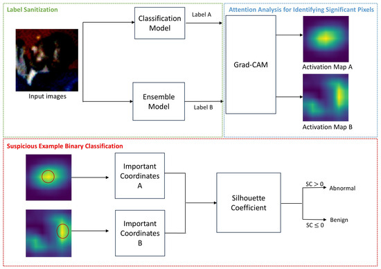
Figure 1. This Flowgraph represents our detection method.

An autoencoder is a generative model designed to compress an input image using an encoder and then reconstruct it using a decoder, making the output as similar to the input as possible. Using this feature, we utilized the Encoder–Decoder architecture of the Vision Transformer, which allows for a patch-based analysis of both the local features and the global context presented within the image. Figure 2 shows the procedure used to train our ensemble model; the architecture of the autoencoder can also be observed.

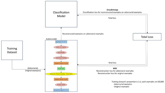
Figure 2. This figure represents our ensemble model’s training procedure.

For the classification model, we selected Mobilenetv2 as a lightweight model and Resnet18 and VGG16 as heavyweight models.

The ensemble model is trained by combining the autoencoder and classification model. The loss function minimizes two objectives: crossentropy for classification and mean squared error (MSE) for reconstruction. As shown in Figure 2, the autoencoder calculates the reconstruction loss, while the classification model computes the classification loss on reconstructed adversarial examples. These loss values are combined, and the training is carried out to minimize the total loss. The classification model was trained to correctly classify the adversarial examples reconstructed by the autoencoder, while the autoencoder was trained to generate images that the classification model can classify correctly.

In conclusion, in Figure 1, the input image is inferred by the classification model to obtain Label A. The ensemble model’s autoencoder reconstructs the input image, and the ensemble model’s classification model infers the reconstructed image to obtain Label B.

3.3. Attention Analysis for Identifying Significant Pixels

This section corresponds to the Attention Analysis for Identifying Significant Pixels presented in Figure 1 and describes the method used to identify and analyze significant pixels. Grad-CAM is used after Label Sanitization to identify significant pixels. This attention-based Explainable AI (xAI) method provides a quick and intuitive way to measure pixel importance during classification [22]. It is represented as follows:

$${\alpha }_k^c={\displaystyle \frac{1}{Z}}\sum _i\sum _j{\displaystyle \frac{\partial y^c}{\partial A_{ij}^k}}$$

(6)

where $y^c$ is the score for class c given the input image I, and $A^k$ represents the activation map k in the last convolutional layer. ${\displaystyle \frac{\partial y^c}{\partial A_{ij}^k}}$ denotes the gradient of $y^c$ with respect to $A^k$. The importance weights ${\alpha }_k^c$ for each activation map k are obtained by averaging these gradients. Z is the size (number of pixels) of $A^k$, and i and j represent the spatial locations in the activation map. These weights are then used to compute a weighted combination of activation maps:

$$L_{\mathrm{Grad-CAM}}^c=\mathrm{ReLU}\left(\sum _k{\alpha }_k^c{A}^k\right)$$

(7)

ReLU is used to highlight features that have a positive influence on the class of interest.

In Figure 1, Label A, predicted by the classification model, and Label B, restored by the ensemble model, are applied to the input image to extract the activation maps. The activation maps are extracted using the Grad-CAM library. In the Grad-CAM tools, the target_layers parameter is used to specify the layer that should be extracted from the classification model, input_tensor represents the input image, and the targets correspond to the label values of the image. In this process, the target_layers used are features[−1] for Mobilenetv2 and VGG16, and layer4[−1] for Resnet18.

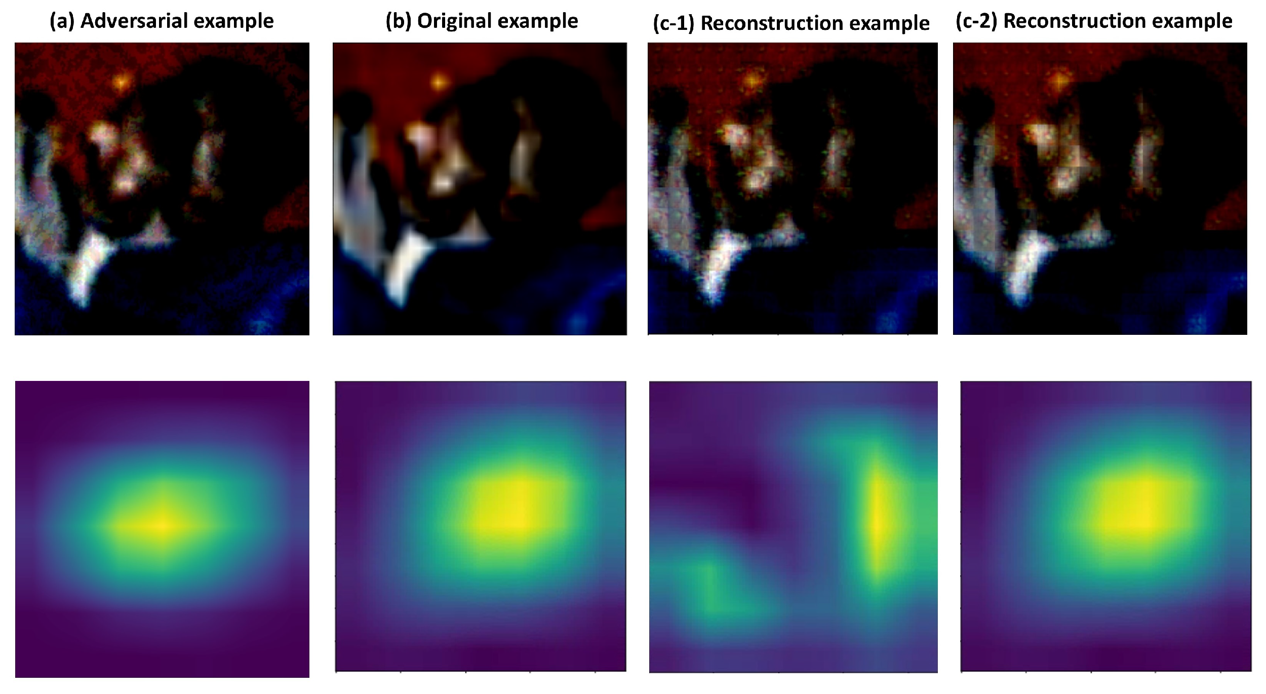
Figure 3 shows examples of the original example, the FGSM adversarial example, and the reconstructed example, and the corresponding activation maps for each. (c-1) shows the reconstructed image and activation map when the input image is adversarial, while (c-2) shows the reconstructed image and activation map when the input image is benign. It can be observed that the significant pixels in the activation map change when the input image is adversarial, whereas the significant pixels remain unchanged when the input image is benign. Specifically, if the Grad-CAM tool is used to extract the activation map after reconstructing (a) example, it results in (c-1). Similarly, if the Grad-CAM tool is used to extract the activation map after the reconstructed (b) example, it results in (c-2). In this process, the target_layers are set to features[−1], the input_tensor corresponds to each example, and the targets are the respective Label A and Label B of each example.

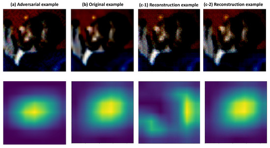
Figure 3. This figure shows samples of the adversarial example, original example, and reconstructed example on Resnet18. (a) indicate the adversarial example obtained using the FGSM and the activation map. (b) is an original example, while (c-1) indicates an example reconstructed using the ensemble model when the input image is adversarial. (c-2) indicates reconstructed examples using the ensemble model when the input image is benign.

3.4. Suspicious Example Binary Classification

This section corresponds to the Suspicious Example Binary Classification shown in Figure 1 and describes the method used for the binary classification of suspicious examples using the extracted significant pixels.

After extracting the activation map, the silhouette coefficient was used to conduct a precise and efficient analysis of whether the positions of significant pixels had changed. For example, in the activation map shown in Figure 1, the light regions contained the most significant pixels. The coordinates of these regions were extracted (N in total) and binary classification was performed based on the silhouette coefficient values.

The silhouette coefficient is a metric used to evaluate the quality of the clusters by comparing the distance between data points within the same cluster and between different clusters. The formula and range for the silhouette coefficient are as follows:

$$s\left(i\right)={\displaystyle \frac{b\left(i\right)-a\left(i\right)}{max\left(a\right(i),b(i\left)\right)}},(-1\le s\le 1)$$

(8)

where $a\left(i\right)$ represents the average distance to all other data points in the same cluster, and $b\left(i\right)$ represents the average distance to all data points in the nearest different cluster. The silhouette coefficient $s\left(i\right)$ ranges from $-1$ to 1, with higher values indicating a better clustering of data points. A negative $s\left(i\right)$ indicates incorrect clustering, a value close to 0 indicates that the data point is on the boundary between clusters, and a value close to 1 indicates well-clustered data points.

Therefore, in this paper, a silhouette coefficient value close to 1 indicates that the positions of significant pixels in the image have changed, suggesting that the image was attacked. A value close to 0 indicates that the positions of significant pixels did not change significantly, suggesting that the image was not attacked. A negative value indicates that the coordinates were mixed, suggesting that the image was not attacked.

In conclusion, in Figure 1, significant pixels were extracted from activation maps A and B, respectively. The key coordinates were selected as the top N locations with the highest importance values in the activation map. By default, 10 coordinates were extracted from each map, though this number can vary depending on the image size. The silhouette coefficient was then calculated for the 20 extracted coordinates, and the presence of an attack was determined based on whether the value was closer to 0 or 1.

Figure 1 shows the flowgraph of the proposed method to prevent adversarial attacks. The ensemble model restores the input image’s label. Using label A of the input image and restored label B, activation maps were extracted through Grad-CAM. From each activation map, the coordinates of the top N most significant pixels were selected, and silhouette coefficients were calculated. If the coefficient was greater than 0, the image was classified as abnormal; otherwise, it was classified as benign.

4. Experiments Results

4.1. Experimental Environment and Dataset

The experiments were conducted in a Desktop environment, utilizing an Intel Core i5 14500 CPU, Nvidia GeForce RTX 4070 Ti SUPER GPU, and 64 GB of RAM.

The autoencoder was first trained using the CIFAR-10 dataset. The images were resized to $224\times 224$, with preprocessing steps including a RandomCrop operation set to padding 4, RandomHorizontalFlip set to its default value, and Normalize using default parameters. The training utilized the Adam optimizer with a learning rate of 0.0001, the model was trained for 20 epochs, and the loss function used was Mean Squared Error (MSE).

Following this, a classification model was fine-tuned on the CIFAR-10 dataset using a pre-trained model from the torchvision.models library, trained on ImageNet. The dataset pre-processing steps were the same as those used for the autoencoder. The classification model was trained using the Adam optimizer, with a learning rate of 0.0001 and 20 epochs, and the loss function employed was Crossentropy. Table 3 shows that Mobilenetv2 achieved a classification performance of 93.76%, Resnet18 achieved 94.98%, and VGG16 achieved 92.85%.

Table 3. This table shows the performance of the fine-tuned classification models.

Model	Performance
Mobilenetv2 [23]	93.76%
Resnet18 [24]	94.98%
VGG16 [25]	92.85%

Subsequently, the trained classification model and autoencoder were combined and further trained as an ensemble model for Label Sanitization. This combined model was trained without freezing the layers, and the dataset pre-processing steps remained consistent with those of the earlier stages. The dataset used for training the ensemble model consisted of both original examples and adversarial examples. Adversarial examples were generated using two attack methods: the FGSM and PGD. The FGSM introduced less sophisticated pixel perturbations, while PGD employed more sophisticated perturbations.

For the ensemble model used in the FGSM version, the training data included 50,000 original training samples and 50,000 FGSM-adversarial training samples. Similarly, for the PGD version, the training data consisted of 50,000 original training samples and 50,000 PGD-adversarial training samples. The parameters for these attacks were configured according to the settings specified in Table 4. Adversarial attacks were implemented using the torchattacks library.

Table 4. This table shows the attack success rates for each model, along with the parameter settings and distance measures for each attack. The attack functions provided by the torchattacks library were used.

Model	Attack Type	Success Rate	Parameter	Distance Measure
Mobilenetv2	FGSM [5]	82.40% (7725/9376)	eps = 8/255	$L_{\infty }$ norm
	PGD [6]	100% (9374/9376)	eps = 8/255, alpha = 2/255, steps = 4	$L_{\infty }$ norm
	C&W [7]	100% (9374/9376)	c = 1, kappa = 0, steps = 50, overshoot = 0.02	$L_2$ norm
	DeepFool [8]	75.73% (7099/9376)	steps = 50, overshoot = 0.02	$L_2$ norm
	BIM [9]	100% (9374/9376)	eps = 8/255, alpha = 2/255, steps = 10	$L_{\infty }$ norm
Resnet18	FGSM [5]	84.01% (7980/9498)	eps = 8/255	$L_{\infty }$ norm
	PGD [6]	100% (9498/9498)	eps = 8/255, alpha = 2/255, steps = 4	$L_{\infty }$ norm
	C&W [7]	100% (9498/9498)	c = 1, kappa = 0, steps = 50, overshoot = 0.02	$L_2$ norm
	DeepFool [8]	65.15% (6188/9498)	steps = 50, overshoot = 0.02	$L_2$ norm
	BIM [9]	100% (9498/9498)	eps = 8/255, alpha = 2/255, steps = 10	$L_{\infty }$ norm
VGG16	FGSM [5]	78.73% (7311/9285)	eps = 8/255	$L_{\infty }$ norm
	PGD [6]	96.91% (8999/9285)	eps = 8/255, alpha = 2/255, steps = 4	$L_{\infty }$ norm
	C&W [7]	100% (9285/9285)	c = 1, kappa = 0, steps = 50, overshoot = 0.02	$L_2$ norm
	DeepFool [8]	84.62% (7857/9285)	steps = 50, overshoot = 0.02	$L_2$ norm
	BIM [9]	97.84% (9085/9285)	eps = 8/255, alpha = 2/255, steps = 10	$L_{\infty }$ norm

The loss function was calculated as the total Loss by combining the crossentropy, used for training the classification model, and MSE, used for training the autoencoder. The Adam optimizer, with a learning rate of 0.0001, was used to jointly train the autoencoder and classification model. The optimizer was applied to the trainable parameters of both models, including the encoder of the autoencoder and the feature extractor and classifier of the classification model. Only parameters with requires_grad = True were selected for optimization to ensure efficient learning. The ensemble model was trained for 20 epochs, and a StepLR scheduler was applied to the optimizer with a step size of 10 and a gamma value of 0.1.

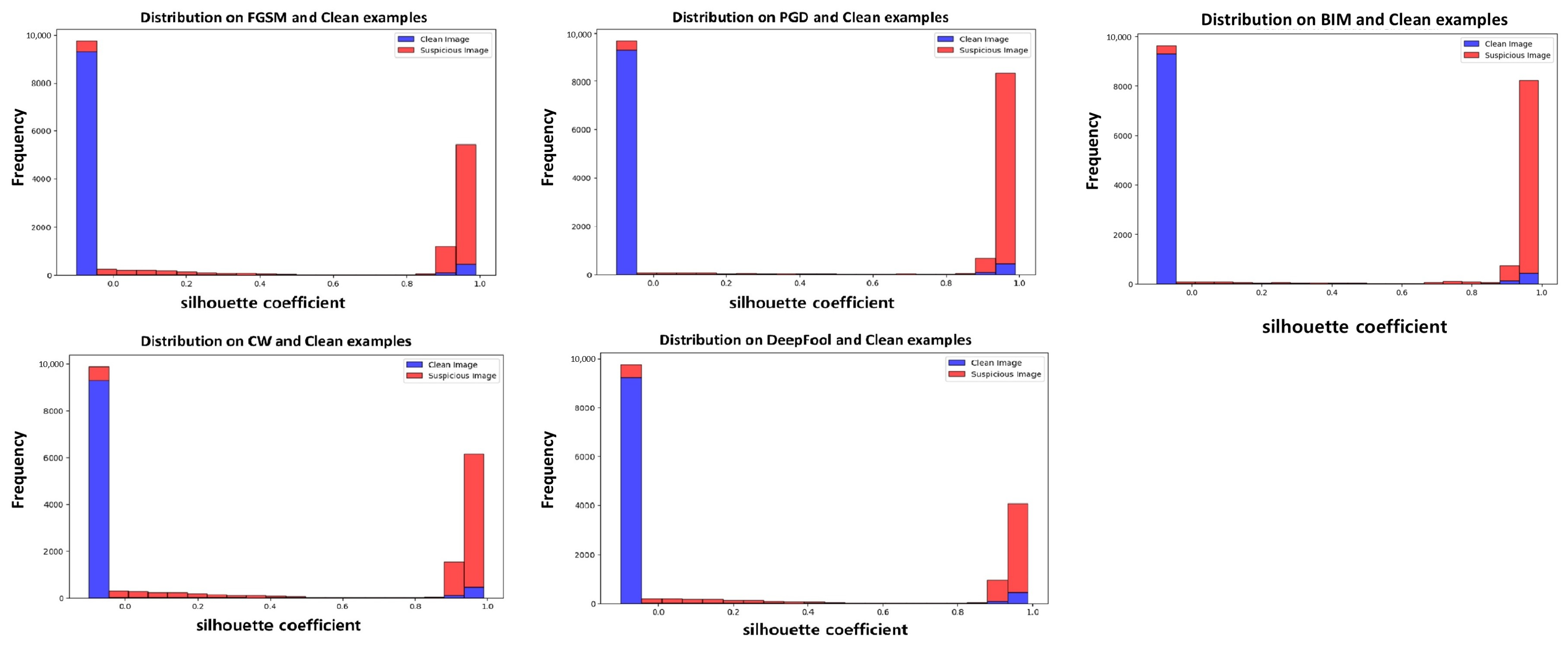
To determine the threshold, a default value was established through experiments. The Resnet18 classification model and the Resnet18_FGSM ensemble model were used, and the silhouette coefficient distributions for five types of adversarial attacks were visualized. The distribution of the silhouette coefficients can be observed in Figure 4. Most original images had silhouette coefficients close to 0, while adversarial examples had coefficients close to 1. Therefore, the default value of the threshold was set to 0.

Figure 4. This figure shows the silhouette coefficient distribution of the dataset used for testing. The classification model that was utilized is Resnet18, while the ensemble model that was used is Resnet18_FGSM. Blue represents original images, and red represents adversarial examples. The x-axis represents the silhouette coefficient values, and the y-axis represents the number of extracted silhouette coefficients.

The attack success rates and parameters of the adversarial attacks are summarized in Table 4. The parameters of the adversarial attacks were set to the default values provided by torchattacks. These are derived by calculating the attack success rate after adversarial attacks were applied to the original examples that the classification models correctly classified. The attack success rates of PGD, C&W, and BIM were high; these rates can vary depending on the parameter settings.

4.2. Evaluation Metrics

The detection performance of the adversarial attack techniques was evaluated through looking at their precision, recall, F1-score, and accuracy.

Precision is the ratio of true positive predictions to the total number of positive predictions made by the model. It indicates how many of the predicted positive samples were actually positive.

$$\mathrm{Precision}={\displaystyle \frac{\mathrm{True}\mathrm{Positives}}{\mathrm{True}\mathrm{Positives}+\mathrm{False}\mathrm{Positives}}}$$

(9)

Recall is the ratio of true positive predictions to the total number of actual positive samples. It indicates how many of the actual positive samples were correctly predicted by the model.

$$\mathrm{Recall}={\displaystyle \frac{\mathrm{True}\mathrm{Positives}}{\mathrm{True}\mathrm{Positives}+\mathrm{False}\mathrm{Negatives}}}$$

(10)

F1-Score is the harmonic mean of precision and recall. It provides a single metric that balances both precision and recall, providing a better measure of the model’s performance, especially when the class distribution is imbalanced.

$$\mathrm{F}1\text{-}\mathrm{Score}=2\times {\displaystyle \frac{\mathrm{Precision}\times \mathrm{Recall}}{\mathrm{Precision}+\mathrm{Recall}}}$$

(11)

Accuracy is the ratio of the number of correct predictions to the total number of predictions. It indicates the overall correctness of the model’s predictions.

$$\mathrm{Accuracy}={\displaystyle \frac{\mathrm{True}\mathrm{Positives}+\mathrm{True}\mathrm{Negatives}}{\mathrm{Total}\mathrm{Predictions}}}$$

(12)

4.3. Adversarial Attack Detection Performance

In this paper, we used FGSM, PGD, C&W, DeepFool, and BIM attacks. We applied each attack to the 10,000 images in the CIFAR-10 test sets and aimed to simultaneously detect both the successfully attacked images and the original test sets.

Table 5 summarizes the experimental results of the proposed method. When applying the detection method to Resnet18, Mobilenetv2, and VGG16, the three models showed similar performance. For the FGSM, Mobilenetv2_PGD showed the highest recall at 0.9339, but, Resnet18_FGSM demonstrated a better F1-score and accuracy, indicating a more balanced detection capability. For the BIM and PGD attacks, which are similar to the FGSM, the method proved effective, with an F1-score and accuracy above 0.9. The Resnet18_FGSM performed best, with an F1-score of 0.9451 and accuracy of 0.9457 for BIM, and an F1-score of 0.9431 and accuracy of 0.9438 for PGD attacks. For C&W and DeepFool attacks, which create perturbations that are difficult for humans to perceive, the heavyweight model VGG16 proved more effective, unlike the results obtained for FGSM-type attacks. VGG16_FGSM achieved the best results, with an F1-score of 0.9291 and accuracy of 0.9367 for DeepFool, and an F1-score of 0.9324 and accuracy of 0.9345 for C&W attacks. These experimental results demonstrate that lightweight models are more effective in detecting FGSM-type attacks, while heavyweight models are more effective in detecting DeepFool and C&W attacks. These results are expected to vary depending on the adversarial examples used in training, and it is anticipated that creating an ensemble model using examples that are applicable to various attacks would enable more effective detection.

Table 5. Detection performance metrics for ensemble models trained on adversarial examples using different attack types. The bold text indicates the best performance for each evaluation metric.

Attack Type	Ensemble Model	Precision	Recall	F1-Score	Accuracy
FGSM	Resnet18FGSM	0.9158	0.9192	0.9175	0.9266
	Resnet18PGD	0.9256	0.8625	0.8929	0.9082
	Mobilenetv2FGSM	0.8676	0.8957	0.8814	0.8950
	Mobilenetv2PGD	0.8987	0.9339	0.9159	0.9253
	VGG16FGSM	0.9072	0.9125	0.9098	0.9236
	VGG16PGD	0.8916	0.8836	0.8876	0.9055
BIM	Resnet18FGSM	0.9311	0.9595	0.9451	0.9457
	Resnet18PGD	0.9406	0.9210	0.9355	0.9332
	Mobilenetv2FGSM	0.8914	0.9248	0.9078	0.9091
	Mobilenetv2PGD	0.9169	0.9572	0.9366	0.9373
	VGG16FGSM	0.9249	0.9243	0.9246	0.9282
	VGG16PGD	0.9129	0.9052	0.9090	0.9138
PGD	Resnet18FGSM	0.9309	0.9557	0.9431	0.9438
	Resnet18PGD	0.9416	0.9377	0.9396	0.9413
	Mobilenetv2FGSM	0.8927	0.9374	0.9145	0.9152
	Mobilenetv2PGD	0.9170	0.9584	0.9372	0.9379
	VGG16FGSM	0.9250	0.9348	0.9299	0.9332
	VGG16PGD	0.9135	0.9214	0.9174	0.9215
DeepFool	Resnet18FGSM	0.8918	0.8974	0.8946	0.9191
	Resnet18PGD	0.9093	0.9024	0.9059	0.9286
	Mobilenetv2FGSM	0.8505	0.8465	0.8485	0.8745
	Mobilenetv2PGD	0.8826	0.8617	0.8720	0.8950
	VGG16FGSM	0.9157	0.9429	0.9291	0.9367
	VGG16PGD	0.9037	0.9360	0.9196	0.9279
C&W	Resnet18FGSM	0.9279	0.9129	0.9203	0.9230
	Resnet18PGD	0.9404	0.9178	0.9289	0.9316
	Mobilenetv2FGSM	0.8887	0.8996	0.8941	0.8969
	Mobilenetv2PGD	0.9134	0.9147	0.9140	0.9167
	VGG16FGSM	0.9273	0.9374	0.9324	0.9345
	VGG16PGD	0.9169	0.9324	0.9245	0.9267

4.4. Comparative Experiment

The comparison experiments included the UNICAD, Feature Squeezing, and Zero-Mean & RGB2BGR methods [11,12,13].

The Feature Squeezing method detects adversarial examples by filtering images before passing them to the classification model, without modifying the existing model. This technique that detects attacks by comparing the model’s prediction results for the original example with its prediction results for the filtered example. This method does not aim to completely block adversarial attacks, but rather to make it more difficult for the attacker to execute the attack. In other words, the attacker may attempt to apply stronger perturbations to bypass the feature squeezing method, which could result in a degradation of image quality, making the image unrecognizable or turning it into an image that appears suspicious due to the attack. The filtering techniques that were used include bit depth reduction, median filtering, and non-local means filtering. For the CIFAR-10 dataset, the best performance was achieved using 5-bit depth reduction, a $2\times 2$ median filter, and a 13-3-2 configuration for non-local means. The median filtering and non-local means were carried out using the ndimage module and the OpenCV library, respectively.

The Zero-Mean method adjusts the brightness of the input image, extracts an activation map using Grad-CAM, and overlays the activation map onto the input image with a weighting factor $\theta$ of 0.1 to create an emphasized image. The classification model then predicts both the input image and the emphasized image. If the predicted labels differ, the input is identified as an adversarial example; if they match, it is classified as an original example. The RGB2BGR method converts the RGB values of the input image to BGR and proceeds with detection in the same way as the Zero-Mean approach. Both detection methods have the limitation that they degrade the performance of the classification model while modifying the image, and they fail to detect when the activation maps of the original example and the adversarial example are very similar.

UNICAD uses the VGG16 model as a feature extractor and selects class-specific prototypes from the CIFAR-10 dataset based on the extracted features. It extracts features from the input images and compares them with the prototypes selected for each class to find the most similar prototype. The method then classifies the images as attack images or clean images according to the detection classification logic. This detection method determines the presence of an attack through a comparison with pre-selected prototypes. However, it relies on the use of a Denoising Autoencoder in the second restoration stage, which may not allow for accurate detection. All suspicious examples from the first detection stage are passed to the second restoration stage. The method used in the first detection stage is applied for restoration using the Denoising Autoencoder. Therefore, if only the detection aspect is measured, there is a possibility that the detection performance may be lower. Although the comparative paper reduced the CIFAR-10 classes to 0–8 and set the 9th class as an unseen class to classify the unseen classes, we set the classes to 0–9 for comparison in this paper and conducted experiments only focusing on the detection aspect.

The evaluation and the dataset used for evaluation were kept the same in our experimental environments. The comparative experiments evaluated the performance of each model individually.

Table 6 presents a comparison of the performance of Mobilenetv2. The most effective method for detecting all attacks was Mobilenetv2_PGD.

Table 6. Comparison of experimental results for Mobilenetv2. The bold text indicates the best performance for each evaluation metric.

Attack Type	Detection Method	Precision	Recall	F1-Score	Accuracy
FGSM	Feature Squeezing [11]	0.6259	0.3431	0.4433	0.6236
	UNICAD [13]	0.4132	0.1047	0.1671	0.5504
	Zero-Mean [12]	0.5868	0.5876	0.5872	0.6716
	RGB2BGR [12]	0.4663	0.3549	0.4031	0.5414
	Mobilenetv2FGSM (Ours)	0.8676	0.8957	0.8814	0.8950
	Mobilenetv2PGD (Ours)	0.8987	0.9339	0.9159	0.9253
BIM	Feature Squeezing [11]	0.8542	0.9931	0.9185	0.9146
	UNICAD [13]	0.5637	0.1605	0.2499	0.5420
	Zero-Mean [12]	0.5265	0.3857	0.4453	0.5768
	RGB2BGR [12]	0.0542	0.0206	0.0299	0.3752
	Mobilenetv2FGSM (Ours)	0.8914	0.9248	0.9078	0.9091
	Mobilenetv2PGD (Ours)	0.9169	0.9572	0.9366	0.9373
PGD	Feature Squeezing [11]	0.8365	0.8673	0.8517	0.8537
	UNICAD [13]	0.4940	0.1158	0.1877	0.5118
	Zero-Mean [12]	0.2040	0.0889	0.1239	0.4461
	RGB2BGR [12]	0.1423	0.0595	0.0840	0.3934
	Mobilenetv2FGSM (Ours)	0.8927	0.9374	0.9145	0.9152
	Mobilenetv2PGD (Ours)	0.9170	0.9584	0.9372	0.9379
DeepFool	Feature Squeezing [11]	0.7757	0.8532	0.8127	0.8458
	UNICAD [13]	0.4502	0.0970	0.1597	0.5025
	Zero-Mean [12]	0.6107	0.7481	0.6725	0.7347
	RGB2BGR [12]	0.6310	0.7835	0.6991	0.7255
	Mobilenetv2FGSM (Ours)	0.8505	0.8465	0.8485	0.8745
	Mobilenetv2PGD (Ours)	0.8826	0.8617	0.8720	0.8950
C&W	Feature Squeezing [11]	0.7471	0.5010	0.5998	0.6765
	UNICAD [13]	0.4625	0.1022	0.1674	0.5055
	Zero-Mean [12]	0.6839	0.7504	0.7157	0.7373
	RGB2BGR [12]	0.6432	0.6467	0.6450	0.6675
	Mobilenetv2FGSM (Ours)	0.8887	0.8996	0.8941	0.8969
	Mobilenetv2PGD (Ours)	0.9134	0.9147	0.9140	0.9167

The Feature Squeezing method demonstrated a strong performance in detecting BIM, PGD, and DeepFool attacks, achieving recall rates of 0.9931, 0.8673, and 0.8532, respectively. This indicates that filtering techniques effectively mitigate the perturbations caused by these attacks. However, the method was less effective against FGSM and C&W attacks. This is because the FGSM and C&W introduce more perturbations to the images, exposing one limitation of Feature Squeezing: its performance degrades when faced with significant perturbations.

The Zero-Mean and RGB2BGR methods demonstrated a relatively good performance in detecting DeepFool and C&W attacks. Compared to other attacks, DeepFool and C&W involve less image perturbation, allowing for effective detection after preprocessing with Zero-Mean and RGB2BGR and generating the emphasized image. However, attacks that cause significant image perturbation, such as the FGSM, PGD, and BIM, were not mitigated by the Zero-Mean or RGB2BGR preprocessing. Furthermore, the generated emphasizing images were not effective in detecting these highly distorted attacks.

UNICAD was presumed to have failed to distinguish between original and adversarial examples during the detection process due to its reliance on the Denoising Autoencoder in the reconstruction stage, which was previously mentioned as a limitation. This dependency likely led to its passing suspicious images without ensuring sufficient accuracy.

Table 7 presents a comparison of Resnet18’s performance. For FGSM-type attacks (FGSM, PGD, and BIM), the Resnet18_FGSM showed the most effective detection performance, with an F1-score of 0.9175, 0.9431, and 0.9451, and accuracies of 0.9266, 0.9438, and 0.9457, respectively. For DeepFool and C&W attacks, Resnet18_PGD was also the most effective in terms of detection.

Table 7. Comparison of the experimental results for Resnet18. The bold text indicates the best performance for each evaluation metric.

Attack Type	Detection Method	Precision	Recall	F1-Score	Accuracy
FGSM	Feature Squeezing [11]	0.6184	0.2988	0.3902	0.6062
	UNICAD [13]	0.4959	0.0984	0.1643	0.5792
	Zero-Mean [12]	0.6600	0.5740	0.6140	0.7106
	RGB2BGR [12]	0.5669	0.5703	0.5686	0.6081
	Resnet18FGSM (Ours)	0.9158	0.9192	0.9175	0.9266
	Resnet18PGD (Ours)	0.9256	0.8625	0.8929	0.9082
BIM	Feature Squeezing [11]	0.8550	0.9168	0.8849	0.8837
	UNICAD [13]	0.6440	0.1445	0.2361	0.5550
	Zero-Mean [12]	0.5389	0.2918	0.3786	0.5765
	RGB2BGR [12]	0.0597	0.0167	0.0261	0.4047
	Resnet18FGSM (Ours)	0.9311	0.9595	0.9451	0.9457
	Resnet18PGD (Ours)	0.9406	0.9210	0.9355	0.9332
PGD	Feature Squeezing [11]	0.8117	0.6704	0.7344	0.7637
	UNICAD [13]	0.6413	0.1384	0.2277	0.5458
	Zero-Mean [12]	0.2711	0.0929	0.1384	0.4886
	RGB2BGR [12]	0.4108	0.2719	0.3273	0.4270
	Resnet18FGSM (Ours)	0.9309	0.9557	0.9431	0.9438
	Resnet18PGD (Ours)	0.9416	0.9377	0.9396	0.9413
DeepFool	Feature Squeezing [11]	0.7383	0.8532	0.7916	0.8359
	UNICAD [13]	0.6481	0.1424	0.2335	0.5477
	Zero-Mean [12]	0.6729	0.7492	0.7090	0.7835
	RGB2BGR [12]	0.6776	0.8233	0.7434	0.7968
	Resnet18FGSM (Ours)	0.8918	0.8974	0.8946	0.9191
	Resnet18PGD (Ours)	0.9093	0.9024	0.9059	0.9286
C&W	Feature Squeezing [11]	0.7371	0.4361	0.5480	0.6496
	UNICAD [13]	0.6532	0.1458	0.2384	0.5495
	Zero-Mean [12]	0.7482	0.7421	0.7452	0.7755
	RGB2BGR [12]	0.7264	0.6992	0.7126	0.7548
	Resnet18FGSM (Ours)	0.9279	0.9129	0.9203	0.9230
	Resnet18PGD (Ours)	0.9404	0.9178	0.9289	0.9316

The Feature Squeezing method, as seen from the results obtained in the comparison with Mobilenetv2, achieved a recall of 0.9168 and accuracy of 0.8837 for BIM, and a recall of 0.8532 and accuracy of 0.8359 for DeepFool. PGD showed a recall of 0.6704 and accuracy of 0.7637, demonstrating a decrease in performance, but still showing decent results.

The Zero-Mean and RGB2BGR methods were effective in detecting DeepFool and C&W attacks. When compared to the results of the lightweight model Mobilenetv2, Zero-Mean showed similar performance in detecting DeepFool and C&W. RGB2BGR, on the other hand, showed an increase in recall of about 0.4 for DeepFool and about 0.5 for C&W. This suggests that the performance of the Zero-Mean and RGB2BGR methods may improve as the model becomes heavier.

The limitations noted for UNICAD were also observed in Resnet18.

Table 8 presents a comparison of the performance of VGG16. For FGSM-type attacks (FGSM, PGD, and BIM), VGG16_FGSM showed the most effective detection performance, with F1-scores of 0.9098, 0.9299, and 0.9246 and accuracies of 0.9236, 0.9332, and 0.9282, respectively. While Feature Squeezing was very effective in detecting BIM and PGD attacks, with recall values of 1.0 and 0.9913, VGG16_FGSM demonstrated a more balanced detection, with F1-scores of 0.9246 and 0.9299.

Table 8. Comparison of experimental results when using VGG16. The bold text indicates the best performance for each evaluation metric.

Attack Type	Detection Method	Precision	Recall	F1-Score	Accuracy
FGSM	Feature Squeezing [11]	0.4999	0.3859	0.4356	0.5762
	UNICAD [13]	0.7081	0.1152	0.1982	0.6384
	Zero-Mean [12]	0.6108	0.5126	0.5574	0.6851
	RGB2BGR [12]	0.5621	0.4250	0.4841	0.6081
	VGG16FGSM (Ours)	0.9072	0.9125	0.9098	0.9236
	VGG16PGD (Ours)	0.8916	0.8836	0.8876	0.9055
BIM	Feature Squeezing [11]	0.7619	1.0000	0.8649	0.8512
	UNICAD [13]	0.8016	0.1388	0.2367	0.5854
	Zero-Mean [12]	0.5835	0.3758	0.4572	0.6123
	RGB2BGR [12]	0.0060	0.0018	0.0028	0.4047
	VGG16FGSM (Ours)	0.9249	0.9243	0.9246	0.9282
	VGG16PGD (Ours)	0.9129	0.9052	0.9090	0.9138
PGD	Feature Squeezing [11]	0.7578	0.9913	0.8590	0.8461
	UNICAD [13]	0.7479	0.0951	0.1688	0.5502
	Zero-Mean [12]	0.1829	0.0592	0.0895	0.4720
	RGB2BGR [12]	0.1407	0.0487	0.0724	0.4270
	VGG16FGSM (Ours)	0.9250	0.9348	0.9299	0.9332
	VGG16PGD (Ours)	0.9135	0.9214	0.9174	0.9215
DeepFool	Feature Squeezing [11]	0.6807	0.9041	0.7767	0.7915
	UNICAD [13]	0.7668	0.1048	0.1844	0.5537
	Zero-Mean [12]	0.6427	0.7809	0.7051	0.7898
	RGB2BGR [12]	0.7168	0.8632	0.7833	0.7968
	VGG16FGSM (Ours)	0.9157	0.9429	0.9291	0.9367
	VGG16PGD (Ours)	0.9037	0.9360	0.9196	0.9279
C&W	Feature Squeezing [11]	0.6239	0.5073	0.5596	0.6155
	UNICAD [13]	0.7617	0.1021	0.1801	0.5526
	Zero-Mean [12]	0.7548	0.8106	0.7737	0.8013
	RGB2BGR [12]	0.7217	0.7631	0.7419	0.7548
	VGG16FGSM (Ours)	0.9273	0.9374	0.9324	0.9345
	VGG16PGD (Ours)	0.9169	0.9324	0.9245	0.9267

The Feature Squeezing method, as seen from the results obtained in the previous comparison, achieved a recall of 1.0000 and accuracy of 0.8512 for BIM, and a recall of 0.9041 and accuracy of 0.7915 for DeepFool. PGD showed a recall of 0.9913 and accuracy of 0.8461, demonstrating an effective performance.

The Zero-Mean and RGB2BGR methods were effective in detecting DeepFool and C&W attacks. When compared to Resnet18, both Zero-Mean and RGB2BGR methods showed an increase of about 0.4 in recall for DeepFool attacks, and an increase about 0.7 in recall for C&W attacks. This supports the earlier estimation that performance improves as the model transitions from lightweight to heavyweight.

The limitations previously observed in UNICAD were also present in VGG16.

In conclusion, our method was proven to be effective in detecting various models and attacks. The Feature Squeezing method was shown to be more effective when the image distortion was lower. The Zero-Mean and RGB2BGR methods demonstrated an increase in detection performance as the model transitioned from lightweight to heavyweight. Although UNICAD did not show a good detection performance, its core use as a Denoising Autoencoder suggests that even if precise detection is not achieved, the recovery performance improves through the use of the Denoising Autoencoder. These results may vary depending on the attack parameters.

4.5. Ablation Study

4.5.1. Analysis of Failure Cases Using the Proposed Method

We presented cases where the proposed method succeeds and we also analyzed the cases of failure.

In Figure 5, a false positive case occurred when the original image was classified as an attacked image. In the activation maps of false positive cases 1 and 2, we can observe a difference between the activation map of the original image and the activation map after Label Sanitization. In this case, false positive case 1 has a silhouette coefficient of approximately 0.9, and false positive case 2 has a silhouette coefficient of 0.5; both of these were detected as attacked images.

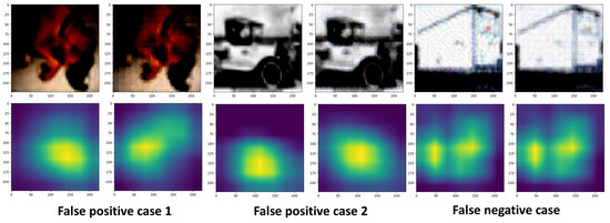
Figure 5. Examples of false positive and false negative cases: this figure shows (from left to right) the original image, reconstructed original image (false positive), FGSM-attacked image, and reconstructed attacked image (false negative).

The false negative case occurred when an attacked image was classified as an original image. In this case, the activation map of the attacked image and the activation map after Label Sanitization appeared identical. This indicates that Label Sanitization did not work as expected, leading to an attacked image being classified as an original image.

These results primarily occurred when the model identified images with similar features. As seen in Figure 5, this included cases such as dogs and trucks. When the model makes its prediction, images of cat and dog, or truck and automobile, share similar features, which leads to activation map differences despite the application of Label Sanitization.

4.5.2. Evaluation of Image Quality Post-Reconstruction

The ensemble model of the proposed method was designed with a focus on Label Sanitization. As a result, a degradation in image quality was inevitable. To identify areas for improvement, the extent of the image quality degradation was measured.

The metric used to evaluate image quality degradation was the SSIM (Structural Similarity Index Measure). The average SSIM was calculated for the evaluation. The evaluation dataset consisted of 10,000 original images, and adversarial examples were selected based on successful attack cases, as shown in Table 4. For example, in the case of the FGSM, the average SSIM was calculated based on 7725 adversarial examples.

The SSIM is a metric used to measure the structural similarity between two images [26]. It considers three main components—luminance (brightness), contrast, and structure—to evaluate the similarities between two images in a way that aligns more closely with the human visual system, rather than relying on pixel-wise differences. The SSIM between two images x and y was calculated using the following formula:

$$SSIM(x,y)={\displaystyle \frac{(2{\mu }_x{\mu }_y+C_1)(2{\sigma }_{xy}+C_2)}{({\mu }_x^2+{\mu }_y^2+C_1)({\sigma }_x^2+{\sigma }_y^2+C_2)}}$$

(13)

${\mu }_x,{\mu }_y$ are the mean luminance of images x and y. ${\sigma }_x,{\sigma }_y$ are the contrast between images x and y. ${\sigma }_{xy}$ is the covariance between images x and y. $C_1,C_2$ are small constants to avoid division by zero in the denominators.

The SSIM values range from 0 to 1, where a value closer to 1 indicates that the two images are more similar. Specifically, SSIM values between 0 and 0.2 indicate severe quality loss, with very little resemblance between images. Values from 0.2 to 0.4 show significant degradation with low similarity. A range of 0.4 to 0.6 represents moderate similarity with noticeable quality loss. Values from 0.6 to 0.8 suggest fairly high similarity with acceptable levels of quality degradation. Finally, values between 0.8 and 1.0 indicate minimal or no visible quality loss, as the images are highly similar.

In Table 9, all ensemble models showed similar SSIM values. For the original image, the SSIM was approximately 0.53, while for the FGSM it was around 0.5, and for the BIM it was approximately 0.51. The SSIM for PGD was around 0.51, for DeepFool it was about 0.53, and for C&W it was about 0.52. In other words, the SSIM values for all ensemble models range from 0.5 to 0.52, indicating a decrease in image quality when the image is reconstructed. The SSIM values ranged between 0.4 and 0.6, indicating noticeable image quality degradation.

Table 9. This table measures the decrease in image quality when reconstructing original and adversarial examples using an ensemble model. Non-attack refers to the original images without any applied attacks.

Attack Type	Ensemble Model	SSIM
Non-Attack	Resnet18FGSM	0.5268
	Resnet18PGD	0.5268
	Mobilenetv2FGSM	0.5266
	Mobilenetv2PGD	0.5266
	VGG16FGSM	0.5267
	VGG16PGD	0.5267
FGSM	Resnet18FGSM	0.5012
	Resnet18PGD	0.5011
	Mobilenetv2FGSM	0.5030
	Mobilenetv2PGD	0.5030
	VGG16FGSM	0.5023
	VGG16PGD	0.5024
BIM	Resnet18FGSM	0.5125
	Resnet18PGD	0.5124
	Mobilenetv2FGSM	0.5110
	Mobilenetv2PGD	0.5110
	VGG16FGSM	0.5106
	VGG16PGD	0.5106
PGD	Resnet18FGSM	0.5114
	Resnet18PGD	0.5113
	Mobilenetv2FGSM	0.5110
	Mobilenetv2PGD	0.5110
	VGG16FGSM	0.5115
	VGG16PGD	0.5115
DeepFool	Resnet18FGSM	0.5353
	Resnet18PGD	0.5347
	Mobilenetv2FGSM	0.5303
	Mobilenetv2PGD	0.5306
	VGG16FGSM	0.5251
	VGG16PGD	0.5240
C&W	Resnet18FGSM	0.5268
	Resnet18PGD	0.5268
	Mobilenetv2FGSM	0.5274
	Mobilenetv2PGD	0.5274
	VGG16FGSM	0.5265
	VGG16PGD	0.5265

These results appear to be a consequence of training the ensemble model with the goal of label sanitization. In our future work, we aim to investigate a framework that can successfully perform label sanitization without degrading the image quality.

4.5.3. Detection Performance Against White-Box Attacks in Real-World Scenarios

Our method was proven effective against white-box attacks through experiments. To verify its effectiveness in real-world scenarios, we evaluated its detection performance against AutoAttack [27]. AutoAttack is a powerful framework designed for assessing adversarial robustness through a combination of four attack techniques. APGD-CE is a gradient-based attack leveraging cross-entropy losses to identify basic vulnerabilities. APGD-DLR employs the Difference of Logits Ratio (DLR) loss to more precisely target weaknesses near decision boundaries. Fast Adaptive Boundary (FAB) performs optimized attacks in the direction closest to the decision boundary, uncovering the most sensitive regions of the model. Finally, Square Attack is a gradient-free attack that uses random search to assess robustness even when gradient information is unavailable. Using AutoAttack, we conducted experiments to determine whether our method is applicable in real-world scenarios.

AutoAttack was implemented using the tool provided by torchattacks, and the parameters were set to their default values. Specifically, the parameters were configured as follows: the norm was set to $L_{\infty }$, eps was 0.3, the version was standard, carrying out the aforementioned four attacks, the number of classes was set to 10, corresponding to the labels in the CIFAR-10 dataset, the seed was set to None, and Verbose was set to False.

Due to the limited computational resources, the evaluation dataset could not be tested on the entire set of examples. Instead, the detection performance was measured using 2500 original examples and 2500 adversarial examples, with a 1:1 ratio. The used for this evaluation dataset was randomly selected.

In Table 10, the proposed method achieved a recall of over 0.93, an F1-score of over 0.91, and an accuracy of over 0.91 across all ensemble models. These results demonstrate that the proposed method can effectively detect adversarial attacks even in real-world scenarios.

Table 10. This table measured the detection performance against AutoAttack.

Attack Type	Ensemble Model	Precision	Recall	F1-Score	Accuracy
AutoAttack	Resnet18FGSM	0.9330	0.9650	0.9488	0.9493
	Resnet18PGD	0.9387	0.9449	0.9418	0.9431
	Mobilenetv2FGSM	0.8907	0.9387	0.9141	0.9147
	Mobilenetv2PGD	0.9140	0.9665	0.9396	0.9400
	VGG16FGSM	0.9290	0.9462	0.9376	0.9393
	VGG16PGD	0.9157	0.9345	0.9250	0.9268

In conclusion, the proposed method is an effective detection approach that works well on various adversarial attacks and models, which demonstrated the ability to effectively detect attacks, even in real-world scenarios.

4.5.4. Execution Time Measurement of Detection Logic

In this section, we measured the execution time of the detection logic to verify its effectiveness in real scenarios. The dataset used for the evaluation was the test dataset. The execution time was measured by repeating the process 100 times with a batch size of 100, and the average time was calculated. In Table 11, the detection logic execution time was measured by representing the average execution time with a ±range based on the standard deviation. This approach quantitatively evaluated the stability of the execution time. These results are shown with error bars in Figure 6.

Table 11. This table shows the execution time of the proposed method.

Ensemble Model	Execution Time
Resnet18FGSM	$84.73\pm 8.81$ ms
Resnet18PGD	$85.38\pm 8.41$ ms
Mobilenetv2FGSM	$169.19\pm 20.72$ ms
Mobilenetv2PGD	$172.45\pm 21.61$ ms
VGG16FGSM	$102.79\pm 5.73$ ms
VGG16PGD	$103.19\pm 5.58$ ms

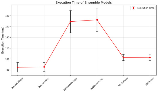
Figure 6. Average execution times (ms) of ensemble models, with error bars showing standard deviations.

Resnet18_FGSM had an execution time of $84.73\pm 8.81$ ms, while Resnet18_PGD had an execution time of $85.38\pm 8.41$ ms, indicating that both models have a low execution time and minimal variability. For Mobilenetv2_FGSM, the execution time was $169.19\pm 20.72$ ms, and Mobilenetv2_PGD had an execution time of $172.45\pm 21.61$ ms, suggesting that these models require longer execution times with moderate variability. VGG16_FGSM model achieved an execution time of $102.79\pm 5.73$ ms, and VGG16_PGD achieved an execution time of $103.19\pm 5.58$ ms, reflecting a balanced execution speed.

These results suggest that the Resnet18 ensemble model was the most efficient and stable in terms of execution time across both detection logics. Mobilenetv2, while effective, incurred the longest execution time, which may impact its real-world applications. VGG16 demonstrated a reasonable execution time, making it potentially suitable for real-world scenarios requiring a balance between speed and stability.

4.6. Discussion

UNICAD exhibited significant differences in its detection performance between original and adversarial samples. Specifically, for the original samples, the performance when using Mobilenetv2 was 0.8875, that using Resnet18 was 0.9275, and that when using VGG16 was 0.9704. However, for adversarial samples, the performance dropped to below 0.2. Additionally, the original-to-adversarial sample ratio used in the tests was not explicitly stated in the referenced paper. To address this, we evaluated the performance using the dataset employed in our study. The results showed an average F1-score of approximately 0.2 and an accuracy of around 0.55.

Our method demonstrated a consistent performance across both lightweight and heavyweight models, such as Resnet18, Mobilenetv2, and VGG16. This indicates that the proposed detection method effectively captures the characteristic differences between original and adversarial examples through clustering analysis using Grad-CAM and silhouette coefficients. Additionally, through an ablation study, we demonstrated that our method can effectively detect adversarial attacks in real-world scenarios.

The results of this study, combined with the explainability, derived based on Grad-CAM, offer users an intuitive understanding of the impact of adversarial attacks during the detection process. This demonstrates the potential to enhance both the transparency and reliability of AI security systems. Furthermore, comparison with existing methods, such as Feature Squeezing and Zero-Mean and RGB2BGR, shows that the proposed approach offers higher versatility and reliability against certain types of attacks.

This contributes significantly to the current research, complementing traditional methods that rely on a single attack type and providing a solution that can be used in various attack scenarios. The results confirm that the proposed method offers a robust solution for adversarial attack detection while maintaining compatibility with the diverse deep learning models.

These findings have significant implications for improving the security and reliability of AI systems across a variety of applications, such as autonomous vehicles, IoT networks, and critical infrastructure protection.

5. Conclusions

This study introduced a new adversarial attack detection and prevention framework, leveraging Grad-CAM and silhouette coefficient-based clustering, and demonstrating its effectiveness through various experiments. Through comprehensive experiments, we verified that the proposed method achieved an F1-score of over 0.90 and high accuracy when tested against various adversarial attacks (FGSM, PGD, BIM, DeepFool, and C&W) on three distinct network architectures (Resnet18, Mobilenetv2, and VGG16). As shown in Table 5, its performance consistently remained high (precision, recall, and accuracy almost exceeded 90% in most scenarios), underscoring the robustness and practical viability of our framework. From these results, the primary findings are summarized as follows:

• The proposed method achieved a high detection performance across a range of deep learning models, including Resnet18, Mobilenetv2, and VGG16, and effectively handled prominent attack types, such as FGSM, PGD, BIM, DeepFool, and C&W.
• Compared to existing approaches like Feature Squeezing and Zero-Mean and RGB2BGR, the framework exhibited higher accuracy and an improved F1-score, showcasing its robustness against diverse attack scenarios.
• Through the ablation study, we showed that the proposed method is effective in real-world scenarios.
• The explainability provided by Grad-CAM enhances the user understanding of adversarial attack effects, contributing to more transparent and reliable AI security systems.

For instance, against PGD—a widely recognized white-box attack—our Resnet18_FGSM ensemble model recorded an F1-score above 0.94, indicating strong detection stability and generalization under stringent attack conditions (see Table 5). Similarly, Mobilenetv2_PGD consistently maintained an accuracy of above 0.92, reinforcing the framework’s adaptability across lightweight and heavyweight architectures.

Despite its contributions, the study has certain limitations. Its computational complexity primarily stems from the use of an ensemble model, which involves simultaneous label restoration and reconstruction processes. This can hinder its real-time application in resource-constrained environments. Furthermore, since our ensemble model focuses on label restoration, the label restoration process may result in image quality degradation, particularly when handling complex adversarial perturbations. This degradation may affect downstream tasks that rely on high-fidelity image reconstruction. Therefore, in future work, the following research directions are suggested:

• Optimization of Ensemble Model Complexity: Simplify the ensemble model architecture to reduce computational overhead while maintaining detection accuracy.
• Improvement in Image Quality: Develop advanced label restoration techniques that preserve image fidelity, ensuring minimal impact on image-dependent downstream tasks.
• Broader Validation: Extend the evaluation to include more datasets, an adaptive threshold configuration, another xAI tool, neural network architectures, and adversarial attack types.
• Integration with Other Defenses: Explore the combination of the proposed framework with existing adversarial defenses to create a more comprehensive and scalable solution.

Through addressing these challenges, the proposed framework has the potential to significantly advance AI security, ensuring its reliability and robustness in real-world environments. Notably, even under severe attack scenarios like BIM and PGD, the detection accuracy remained above 0.93 (Table 5). These findings suggest that the proposed method could offer reliable security safeguards for real-time, mission-critical applications—such as autonomous driving, IoT environments, or critical infrastructure protection—where adversarial robustness is paramount.

References

- Asgari Taghanaki, S.; Das, A.; Hamarneh, G. Vulnerability analysis of chest x-ray image classification against adversarial attacks. In Proceedings of the Understanding and Interpreting Machine Learning in Medical Image Computing Applications: First International Workshops, MLCN 2018, DLF 2018, and iMIMIC 2018, Held in Conjunction with MICCAI 2018, Granada, Spain, 16–20 September 2018; Proceedings 1. Springer: Berlin/Heidelberg, Germany, 2018; pp. 87–94. [Google Scholar]
- Alparslan, Y.; Alparslan, K.; Keim-Shenk, J.; Khade, S.; Greenstadt, R. Adversarial attacks on convolutional neural networks in facial recognition domain. arXiv 2020, arXiv:2001.11137. [Google Scholar]
- Zhang, H.; Wang, J. Towards adversarially robust object detection. In Proceedings of the IEEE/CVF International Conference on Computer Vision, Seoul, Republic of Korea, 27–28 October 2019; pp. 421–430. [Google Scholar]
- Chernikova, A.; Oprea, A.; Nita-Rotaru, C.; Kim, B. Are self-driving cars secure? evasion attacks against deep neural networks for steering angle prediction. In Proceedings of the 2019 IEEE Security and Privacy Workshops (SPW), San Francisco, CA, USA, 20–22 May 2019; IEEE: New York, NY, USA, 2019; pp. 132–137. [Google Scholar]
- Goodfellow, I.J.; Shlens, J.; Szegedy, C. Explaining and harnessing adversarial examples. arXiv 2014, arXiv:1412.6572. [Google Scholar]
- Madry, A.; Makelov, A.; Schmidt, L.; Tsipras, D.; Vladu, A. Towards deep learning models resistant to adversarial attacks. arXiv 2017, arXiv:1706.06083. [Google Scholar]
- Carlini, N.; Wagner, D. Towards evaluating the robustness of neural networks. In Proceedings of the 2017 IEEE Symposium on Security and Privacy (sp), San Jose, CA, USA, 22–26 May 2017; IEEE: New York, NY, USA, 2017; pp. 39–57. [Google Scholar]
- Moosavi-Dezfooli, S.M.; Fawzi, A.; Frossard, P. Deepfool: A simple and accurate method to fool deep neural networks. In Proceedings of the IEEE Conference on Computer Vision and Pattern Recognition, Las Vegas, NV, USA, 27–30 June 2016; pp. 2574–2582. [Google Scholar]
- Kurakin, A.; Goodfellow, I.J.; Bengio, S. Adversarial examples in the physical world. In Artificial intelligence Safety and Security; Chapman and Hall/CRC: Boca Raton, FL, USA, 2018; pp. 99–112. [Google Scholar]
- Su, J.; Vargas, D.V.; Sakurai, K. One pixel attack for fooling deep neural networks. IEEE Trans. Evol. Comput. 2019, 23, 828–841. [Google Scholar] [CrossRef]
- Xu, W. Feature squeezing: Detecting adversarial exa mples in deep neural networks. arXiv 2017, arXiv:1704.01155. [Google Scholar]
- Ye, D.; Chen, C.; Liu, C.; Wang, H.; Jiang, S. Detection defense against adversarial attacks with saliency map. Int. J. Intell. Syst. 2022, 37, 10193–10210. [Google Scholar] [CrossRef]
- Pellcier, A.L.; Giatgong, K.; Li, Y.; Suri, N.; Angelov, P. UNICAD: A unified approach for attack detection, noise reduction and novel class identification. In Proceedings of the International Joint Conference on Neural Networks (IJCNN), Yokohama, Japan, 30 June–5 July 2024. [Google Scholar]
- Akhtar, N.; Mian, A. Threat of adversarial attacks on deep learning in computer vision: A survey. IEEE Access 2018, 6, 14410–14430. [Google Scholar] [CrossRef]
- Zheng, Z.; Hong, P. Robust detection of adversarial attacks by modeling the intrinsic properties of deep neural networks. Adv. Neural Inf. Process. Syst. 2018, 31, 7924–7933. [Google Scholar] [CrossRef]
- Carrara, F.; Falchi, F.; Caldelli, R.; Amato, G.; Becarelli, R. Adversarial image detection in deep neural networks. Multimed. Tools Appl. 2019, 78, 2815–2835. [Google Scholar] [CrossRef]
- Li, Y.; Angelov, P.; Suri, N. Adversarial attack detection via fuzzy predictions. IEEE Trans. Fuzzy Syst. 2024, 32, 7015–7024. [Google Scholar] [CrossRef]
- Szegedy, C.; Zaremba, W.; Sutskever, I.; Bruna, J.; Erhan, D.; Goodfellow, I.; Fergus, R. Intriguing properties of neural networks. arXiv 2013, arXiv:1312.6199. [Google Scholar]
- Papernot, N.; McDaniel, P.; Jha, S.; Fredrikson, M.; Celik, Z.B.; Swami, A. The limitations of deep learning in adversarial settings. In Proceedings of the 2016 IEEE European Symposium on Security and Privacy (EuroS&P), Saarbrücken, Germany, 21–24 March 2016; IEEE: New York, NY, USA, 2016; pp. 372–387. [Google Scholar]
- Moosavi-Dezfooli, S.M.; Fawzi, A.; Fawzi, O.; Frossard, P. Universal adversarial perturbations. In Proceedings of the IEEE Conference on Computer Vision and Pattern Recognition, Honolulu, HI, USA, 21–26 July 2017; pp. 1765–1773. [Google Scholar]
- Baluja, S.; Fischer, I. Adversarial transformation networks: Learning to generate adversarial examples. arXiv 2017, arXiv:1703.09387. [Google Scholar]
- Selvaraju, R.R.; Cogswell, M.; Das, A.; Vedantam, R.; Parikh, D.; Batra, D. Grad-cam: Visual explanations from deep networks via gradient-based localization. In Proceedings of the IEEE International Conference on Computer Vision, Venice, Italy, 22–29 October 2017; pp. 618–626. [Google Scholar]
- Sandler, M.; Howard, A.; Zhu, M.; Zhmoginov, A.; Chen, L.C. Mobilenetv2: Inverted residuals and linear bottlenecks. In Proceedings of the IEEE Conference on Computer Vision and Pattern Recognition, Salt Lake City, UT, USA, 18–23 June 2018; pp. 4510–4520. [Google Scholar]
- He, K.; Zhang, X.; Ren, S.; Sun, J. Deep residual learning for image recognition. In Proceedings of the IEEE Conference on Computer Vision and Pattern Recognition, Las Vegas, NV, USA, 27–30 June 2016; pp. 770–778. [Google Scholar]
- Simonyan, K.; Zisserman, A. Very deep convolutional networks for large-scale image recognition. arXiv 2014, arXiv:1409.1556. [Google Scholar]
- Wang, Z.; Bovik, A.; Sheikh, H.; Simoncelli, E. Image quality assessment: From error visibility to structural similarity. IEEE Trans. Image Process. 2004, 13, 600–612. [Google Scholar] [CrossRef] [PubMed]
- Croce, F.; Hein, M. Reliable evaluation of adversarial robustness with an ensemble of diverse parameter-free attacks. In Proceedings of the International Conference on Machine Learning, PMLR, Virtual, 13–18 July 2020; pp. 2206–2216. [Google Scholar]
Disclaimer/Publisher’s Note: The statements, opinions and data contained in all publications are solely those of the individual author(s) and contributor(s) and not of MDPI and/or the editor(s). MDPI and/or the editor(s) disclaim responsibility for any injury to people or property resulting from any ideas, methods, instructions or products referred to in the content. |
© 2025 by the authors. Licensee MDPI, Basel, Switzerland. This article is an open access article distributed under the terms and conditions of the Creative Commons Attribution (CC BY) license (https://creativecommons.org/licenses/by/4.0/).