Article

Wastewater Infrastructure as a Public Health Tool: Agent-Based Modeling of Surveillance Strategies in a COVID-19 Context

1
Department of STEM Education, College of Education, University of Kentucky, Lexington, KY 40506, USA
2
WWAMI School of Medical Education, College of Health, University of Alaska Anchorage, Anchorage, AK 99504, USA
3
Department of Mechanical and Aerospace Engineering, Pigman College of Engineering, University of Kentucky, Lexington, KY 40506, USA
*
Author to whom correspondence should be addressed.
Systems 2025, 13(12), 1093; https://doi.org/10.3390/systems13121093
Submission received: 9 September 2025 / Revised: 10 November 2025 / Accepted: 25 November 2025 / Published: 3 December 2025
(This article belongs to the Special Issue System Dynamics Modeling and Simulation for Public Health)

Abstract

Wastewater-based epidemiology (WBE) played a vital role during the COVID-19 pandemic by providing early warnings of outbreaks through SARS-CoV-2 RNA detection in sewage. Many rural communities did not benefit from WBE because limited centralized sewer infrastructure challenged conventional WBE surveillance strategies. We present a multi-agent computer model simulating COVID-19 spread in a U.S. county with both sewered and non-sewered zones to assess the performance of WBE in this setting. We evaluate how the sewage service status of the first SARS-CoV-2 carrier, cross-zone community mobility, and WBE detection thresholds influence outbreak detection timing at the county’s wastewater treatment plant under basic reproduction numbers (R0) of 4 and 8. Our key findings include that (1) a detection threshold of 10 gc/mL can identify outbreaks up to six days earlier than a threshold of 50 gc/mL; (2) outbreaks originating in non-sewered zones are detected 1–2 days later, compared with outbreaks in sewered zones; and (3) cross-zone community mobility impacts detection timing only when outbreaks begin in non-sewered zones. Furthermore, once detected, disease prevalence can increase by five- to eleven-fold within the following week. These results underscore the importance of WBE sensitivity and tailored surveillance strategies in both sewered and non-sewered zones of a community. Strengthening WBE capabilities at local treatment facilities can improve early outbreak detection, thereby supporting timely public health interventions.

1. Introduction

Wastewater-based epidemiology (WBE) tracks pathogens in sewage and wastewater, especially those transmitted through the waterborne or fecal-oral routes [1,2]. Complementary to the clinical surveillance that may identify symptomatic clinical cases, hospitalizations, or deaths, WBE may detect the presence and transmission of pathogens at the community level, even in the absence of symptoms, access to healthcare, or health-seeking behaviors [1,2,3].
The use of WBE can be traced back to the mid-1800s [4]. Since the 1970s, this approach has been widely implemented to help eradicate poliovirus globally [5,6]. Along with the extensive use of the Polymerase Chain Reaction (PCR) and its associated techniques, such as reverse transcription PCR (RT-PCR) and quantitative PCR (qPCR), researchers have detected pathogens from at least 24 viral families in wastewater [1]. Therefore, it is unsurprising that WBE detection was deployed to surveil the spread of COVID-19 from the beginning of the pandemic. The findings on the fecal shedding of SARS-CoV-2 among patients [7] and the persistence of SARS-CoV-2 RNA in wastewater [8] further support the applicability of WBE in this context.
Studies have demonstrated that WBE detection may provide early warnings to public health officials regarding the presence and transmission of COVID-19 in sewered communities, allowing critical lead time for action, particularly since COVID-19 vaccines were unavailable until the end of 2020 [2]. For example, by comparing the concentrations of SARS-CoV-2 RNA in primary sewage sludge in the New Haven, Connecticut, USA, with the clinic testing results and the local COVID-19 hospital admissions, Peccia et al. [9] found the changes in SARS-CoV-2 RNA concentrations appeared 0–2 days ahead of the percentage of positive tests by date of specimen collection, 1–4 days ahead of local hospital admissions, and 6–8 days ahead of the publicly reported positive test results for SARS-CoV-2. A more extensive systematic review of 92 studies on wastewater surveillance for COVID-19, conducted from January 2020 to May 2021, summarized that 13 studies reported positive detections in wastewater before the first community cases were detected, and at least 50 studies reported an association between viral load and community cases [3].
Despite its ability to provide authorities with critical lead time during outbreaks like COVID-19, WBE indicators are only valuable when testing is not delayed [10]. However, many rural areas that lack testing capacity face challenges in receiving timely results, as samples must be transported to testing labs. WBE’s effectiveness also depends on regional infrastructure. In areas with both sewered (i.e., homes connected to public sewer systems) and non-sewered zones (decentralized wastewater systems not connected to public sewer systems, such as septic tanks, pit latrines, etc.), outbreaks in non-sewered regions may go undetected, increasing the risk of transmission. This risk is especially high in communities where frequent interactions occur between populations across different wastewater service systems [11,12]. Therefore, understanding the infection spread patterns in these areas will help elucidate the extent to which WBE processes, both performed through centralized labs and local mobile laboratories, may improve the public health responses in such rural settings.
In recent decades, agent-based models (ABMs) have emerged as a powerful tool for exploring system outcomes by capturing the extensive interactions among numerous elements, in both epidemiology and water science [13,14,15,16]. By defining interactions among individual agents and incorporating variables relevant to the scenarios of interest, ABMs have helped guide targeted public health interventions by simulating different situations and shedding light on the dynamics of disease transmission, including COVID-19 [13,15]. In water science, ABMs have been applied to facilitate the understanding of water system dynamics, inform water management decision-making, and inspire interdisciplinary studies at both the micro- and macroscale [16]. Specifically, the application of ABMs in the field of wastewater treatment has enabled researchers to measure the heterogeneous bacterial reactions and interspecies reactions in wastewater to enhance the systems, such as the biological phosphorus removal system, and physical structures in wastewater treatment plants [17].
Since the COVID-19 pandemic, several research groups have developed ABMs that link models of infectious disease transmission, community population characteristics, viral load data, and wastewater data to enhance the application of WBE in facilitating successful public health initiatives, strategies, and action plans. Fazli et al. [18] developed three stochastic models that integrate a susceptible-exposed-infected-recovered (SEIR) model, viral load in wastewater, and the COVID-19 case count, and compared the forecasting quality of these models. Their results suggest that the SEIR model based on viral load data can reliably predict the number of infections in outbreaks. DelaPaz-Ruíz et al. [19] developed an ABM integrating three submodels—disease spread, population mobility, and wastewater production—to simulate COVID-19 outbreaks and wastewater infection levels within a sewered community, which provided a comprehensive means to track outbreak dynamics and visualize spatiotemporal maps of infected wastewater flow in a wastewater system. Recent work from a research team in Germany [20,21] developed an ABM that further integrated infection dynamics, viral shedding curves, and a hydrologic model of sewage flow to investigate the effect of sampling protocols, precipitation infiltration, viral decay, normalization strategies, and intervention timing on infection dynamics. Their modeling results suggest that wastewater-based surveillance data can serve as an early epidemiological indicator to facilitate outbreak prediction. Overall, these studies expand our understanding of the potential of using wastewater data to surveil the spread of infectious diseases by integrating increasingly comprehensive information into ABMs at both temporal and spatial scales. However, all of them focus on the areas with full sewage service. In the USA, approximately 20% of the population is not connected to a centralized sewage system [22]. In many regions, such as the one simulated in this study, these people may live adjacent to those connected to a centralized sewage system and interact socially. Therefore, it is important to understand the performance of WBE in such regions to design effective WBE strategies.
In this study, we developed a multi-agent wastewater-based epidemiology model (hereinafter referred to as the WBE model) to explore the possible transmission patterns of COVID-19 within Boyd County, Kentucky, a U.S. county of 48,447 inhabitants, which comprises a mixture of sewered and non-sewered zones. The WBE model focuses on simulating the dynamics of the COVID-19 epidemic originating from either the sewered or non-sewered zones in this county. At the county level, it integrates an SEIR epidemic model with GIS data of county sewage systems, county population demographics, social networks (such as households, schools, workplaces, and communities), population mobility, and clinic viral loads to simulate the daily and cumulative prevalence of COVID-19 during the early stage of outbreaks (i.e., the first 60 days), with a low quarantine rate and no vaccination. Using the model, we evaluated how the rates of community travel between sewered and non-sewered zones (hereinafter referred to as the cross-zone travel) and the sewage service status of the first SARS-CoV-2 carrier (i.e., non-sewered vs. sewered) influence the spread of COVID-19 under varying transmission levels and how different WBE detection thresholds may impact the detection timing. Specifically, we selected R0 values of 4 and 8 to represent moderate and high transmission scenarios and used detection thresholds of 10 gc/mL and 50 gc/mL as the lower and upper bounds of SARS-CoV-2 WBE assay sensitivity [23]. Additionally, we examined the cumulative prevalence progress if detection is delayed by transporting the wastewater sample to a centralized lab, which may take multiple days, especially when shipping from rural/remote regions. In this article, we present the development of the WBE model and the modeling results that answer the following questions:
(1)
At the basic reproduction numbers (R0) of 4 and 8, how do the WBE detection sensitivity, sewage service status of the first SARS-CoV-2 carrier, and the cross-zone travel rate affect the number of days required for the viral concentration in the aggregated wastewater at the local wastewater treatment plant to reach the predefined WBE detection threshold?
(2)
At the basic R0 of 4 and 8, how do the WBE detection sensitivity, sewage service status of the first SARS-CoV-2 carrier, and the cross-zone travel rate affect the cumulative COVID-19 prevalence when the predefined WBE threshold is reached?
(3)
At the basic R0 of 4 and 8, how do the respective cumulative prevalences progress in the seven days after the WBE threshold is reached in the simulated county?

2. Materials and Methods

2.1. WBE Model Development

The WBE model (Figure 1) was developed using NetLogo 6.4 [24], a multi-agent modeling environment designed for agent-based models. Building on a susceptible-exposed-infectious-recovered (SEIR) epidemic model that simulates the transmission and progression of infectious diseases [25], we integrated GIS information, population mobility, social networks, and wastewater surveillance components to simulate COVID-19 transmission dynamics driven by interpersonal interactions in Boyd County, Kentucky, USA. We selected this county due to its diverse wastewater infrastructure, combination of rural and semi-urban environments, and availability of detailed GIS data. Within the county, two wastewater treatment plants handle the pooled wastewater from most of the cities that provide sewage services within their respective limits, with a minority portion of the sewage (the blue region in Figure 1) transferred to a treatment plant in an adjacent county. However, many areas of the county still rely on septic tanks for wastewater management. The spatial proximity and social connections between the sewered and non-sewered regions allow frequent interactions among residents in these areas.
Below, a detailed model summary is provided following the Overview, Design concepts and Details (ODD) protocol [26] to describe the model development and the key components.

2.1.1. Purpose

The WBE model simulates the transmission patterns of COVID-19 in a U.S. county that encompasses both sewered and non-sewered zones. Specifically, this WBE model aimed to represent the spread of SARS-CoV-2 within the county during the early stage of an outbreak to gain insights into how community mobility, sewage service status (non-sewered vs. sewered), and WBE detection sensitivity affect outbreak detection timing and the associated disease prevalence at different basic reproduction numbers (R0).

2.1.2. Entities, State Variables, and Scales

The model used three types of agents: land patches, houses, and humans. Land patches mapped the county and defined key properties of the population, such as population density and geographic distribution, in the simulated county. A total of 16,105 patches represent 15 county census tracts in the model based on the GIS census tract boundary data. Each patch represents an area of 163 by 163 square meters. We overlaid county sewage system GIS data on the census tracts [27] to accurately locate the sewage system in the model. All the GIS data were measured in QGIS 3.30 [28].
Household and population data from the 2021 American Community Survey [29] were used to create and distribute household and human agents within the census tracts in the model, resulting in a total of 18,251 household agents and 48,447 human agents. The sewage service status and number of household members were defined for each house agent based on their geographic locations. The state variables of human agents fell into three categories: geographic location, disease transmission, and social network (Table 1), allowing us to observe disease spread patterns in the human population through four different networks: family, school, workplace, and community. Each time step of the WBE model represented one day.

2.1.3. Initialization and Input

Figure 2 illustrates the initiation process of the WBE model. The GIS data of census tracts [27] and the county’s sewage system defined county tract boundaries and sewage system configuration. We considered tracts within city limits as fully sewered and applied a sewage coverage of 80% [22] to the tracts where not all households were sewered, resulting in 90–91% sewage coverage in the county. Next, the household and population data from the 2021 American Community Survey [29] informed the distribution of the human agents and established their social networks within the county. An exposed agent, i.e., a carrier, was then introduced into the model to initiate an outbreak.

2.1.4. Process Overview and Scheduling

At each time step (i.e., one day), the model procedure followed people’s typical daily activities, determined by their age, mobility, employment, social network, and disease status. These activities happened in a predefined order, as specified below.
  • Wastewater surveillance: The aggregated wastewater from the previous day was sampled and tested at the county’s wastewater treatment plant to measure the concentration of SARS-CoV-2 RNA copies.
  • Quarantine: The model examined the status of infectious agents and updated their quarantine status according to a defined quarantine rate.
  • Travel: Based on the defined community traveling rate, a portion of human agents aged 18–74 traveled across the sewered and non-sewered zones or within the sewered or non-sewered zones for reasons such as shopping, visiting friends, entertainment, etc. These travels are distinct from school and work activities. Cross-zone travel rates were varied as a part of our analysis to examine the effect of this variable.
  • Disease transmission through social networks: An SEIR compartmental model simulated SARS-CoV-2 viral transmission and disease progression. During this process, human agents contacted others through four social networks. Specifically, agents contacted family members, community members (i.e., other human agents on the same patch but excluded from family), classmates, and human agents in their workplace networks. During weekdays (Monday through Friday), PreK-college students (aged 0–17 and aged 18–64 enrolled in college) and workers (aged 18–64 and employed) also interacted with their classmates or colleagues. Exposed and unquarantined infectious individuals may transmit SARS-CoV-2 viruses to their susceptible contacts, based on a transmission rate defined for each network. The disease states of individual agents were updated after each interaction.
  • Travel: Human agents who traveled in step 2 returned home.
  • Iterating the model: The overall population disease status and simulated dates were updated.

2.1.5. Design Concepts

Emergence: Three emergent properties were elucidated by this model: the population prevalence, epidemic duration, and SARS-CoV-2 RNA concentration at the county’s primary wastewater treatment plant (i.e., the green region in Figure 1). The population prevalence and epidemic duration emerged from the interactions among human agents in the simulated population, and the viral RNA concentrations in the wastewater treatment plant resulted from the disease spread and virus fecal shedding within the population.
Interaction: The SEIR compartmental model defined the interactions related to disease spreading and progress (see Section 2.1.6 for details). These interactions occurred through four social networks: family, school, workplace, and community. For each agent, the members of the first three networks remained relatively stable in each test, while the members of their community network could vary daily due to population mobility.
Stochasticity: The WBE model comprised four submodels: social networks, disease transmission, population mobility, and wastewater surveillance (see Section 2.1.6 for details). All four submodels encompassed stochastic elements. To establish family and community networks, human agents were first assigned to households semi-randomly due to the lack of detailed family census data. Then, school-age agents and adult employed agents were assigned to school or workplace networks, also in a semi-random manner. While the total number of contacts in these networks remained the same, the composition of the family, community, school, or workplace network for each human agent varied in each test.
For disease transmission, network-specific probabilities were defined based on the tested R0 value. Both the incubation period and disease period varied among human agents, with the standard deviation of 1 day and 2 days, respectively. The quarantine status was randomly assigned to the infectious agents based on a defined quarantine rate. Population mobility was also influenced by defined probabilities and randomness. Based on the changing rates of mobility in the population mobility data [30], people who were traveling were randomly selected from the unquarantined adult agents and moved to a random county patch that contained at least one other person. In the wastewater surveillance submodel, exposed and infectious agents were randomly designated to shed virus in their stool for 21 days based on a defined shedding probability.
Observation: The model generated various system outputs, including daily new cases, COVID-19 cumulative prevalence, epidemic duration, and SARS-CoV-2 RNA concentration in wastewater. We were specifically interested in observing these outputs when the epidemic was initiated in a sewered zone vs. a non-sewered zone. We also examined the changes in cumulative prevalence over the week following the day when the viral RNA concentrations reached the predefined threshold in the wastewater treatment plant. These outputs provided insight into the impact of surveillance testing time lags on the spread of COVID-19 in the early stage of an outbreak.

2.1.6. Submodels

Social networks: The present model incorporated four types of social networks—family, school, workplace, and community—following the processes and categories established in existing studies on social networks [31,32,33]. Using household and population data, we distributed 48,447 people into 18,251 households to establish the family network based on age. Each household was assigned 1–7 members, with at least one adult member. The school networks included individuals aged 0–17 years (i.e., PreK-12 students) and those aged 18–64 who were enrolled in college (i.e., college students). The toddlers (aged 0–4) were placed in daycare or preschool networks, with up to 10 daily contacts. The primary/secondary school-aged children (aged 5–17) were assigned to K-12 school networks with up to 25 daily contacts. College students (aged 18–64 and enrolled in college) were assigned to college networks with up to 25 daily contacts. Employed adults (aged 18–64) were assigned to workplace networks with up to 13 contacts per day. Adults working across networks, such as teachers, were assigned to workplace networks due to a lack of detailed data. In addition to these three structured networks, people on the same patch on a given day formed a community network with up to 13 daily contacts, as established in existing studies [31,33].
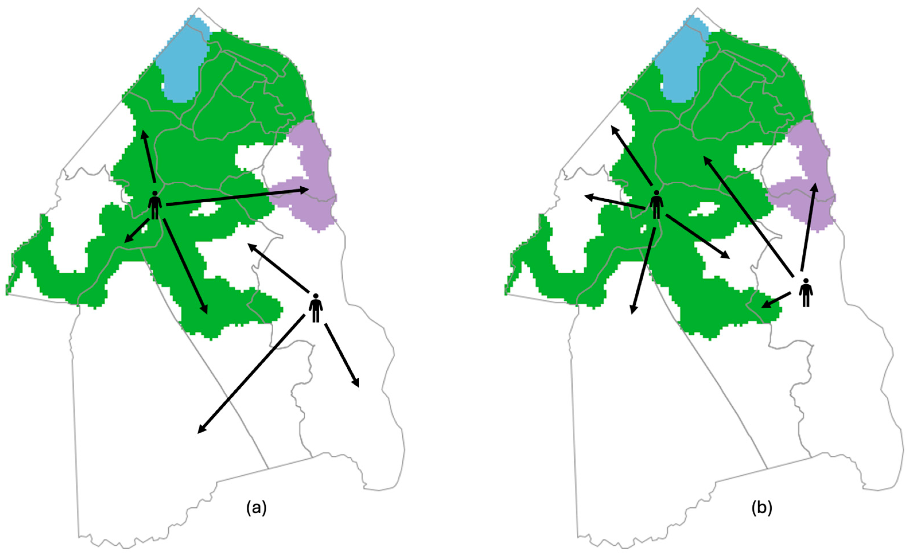
Population Mobility: People’s daily traveling activities can be complex. In this model, we primarily focused on travel related to community networks, as interactions within family, school, and workplace networks were assumed to be relatively stable over short periods, such as 6 to 12 months. To explore the impact of disease initiated from sewered versus non-sewered zones on epidemic development, we differentiated the travel occurring within the same zone type (within-zone travel) and travel across two different zone types (cross-zone travel) (Figure 3). The Google Community Mobility Reports [30] suggested population mobility could change up to 25% between weekdays and holidays. Therefore, we use 25% as the maximum percentage of adults who travel within the sewered or non-sewered zone. Considering that about 90% of the population was sewered in the model, we capped the cross-zone traveling at 10%.
During within-zone travel and cross-zone travel, selected agents physically moved from one patch to another patch with at least one other human agent. This travel enabled agents to contact agents outside their immediate community (e.g., neighborhoods), resulting in broader social mixing. A travel rate of 0% means that no agents physically move in the model. Agent contacts related to workplace and school interactions are embedded within the corresponding social networks and do not require the agent to physically travel in the model. Therefore, when travel parameters are disabled in the WBE model, disease can still spread through social networks. Disease spread can only be completely stopped by adjusting the transmission rate parameters to zero.
Disease transmission: The SEIR framework (Figure 4) has been used in multiple studies for modeling WBE, including both equation-based compartmental models [34,35,36] and agent-based models [18,20]. In this study, we employed the SEIR framework, following a similar structure to that of existing agent-based epidemic models, to simulate disease transmission. Namely, a susceptible agent becomes an exposed agent if it is infected in a social interaction (S->E); an exposed agent progresses to the infectious stage after an incubation period (E->I); and an infectious agent either recovers or dies after experiencing a disease period (I->R). In the present model, parameters specific to the original strain of SARS-CoV-2, including the incubation period, the disease period, the infectious period, and mortality, were utilized to simulate the spread patterns of this disease (Table 2). Quarantine and vaccination parameters were also incorporated into the model with the assumption that quarantined agents do not infect others and vaccinated agents are not susceptible to COVID-19. In this WBE model, the infectious period starts from the last 2 days of the incubation period and lasts through the disease period [37].
The basic reproduction number (R0) of SARS-CoV-2 was used to determine the transmission probabilities in this model because R0 can be derived from the transmissibility of the pathogen, contact rate, and the duration of infectiousness [38]. The relationship can be represented using Equation (1).
R0 = c × p × d
where c is the contact rate, p is the transmissibility of the pathogen, and d is the duration of infectiousness.
In the current WBE model, Equation (1) was converted into Equation (2).
p = R0/(c × d)
Using the contacts defined in the social networks and the infectious period, we determined the transmission rate to set up a theoretical R0 for each social network. The R0 of SARS-CoV-2 differed by virus variant. The estimated R0 value of the original strain was 3.38 ± 1.40 [39], the Delta variant had an estimated R0 of 5.08 [40], and the Omicron variant had an estimated R0 of 8.2 [41]. Based on this range, we selected R0 values of 4 and 8 to represent moderate to severe transmission situations.
Wastewater Surveillance: Equation (3) was used to estimate the daily concentration of viral copies in aggregated wastewater at the county’s wastewater treatment plant.
Concv = (Mf × Vf × Nsv)/(Df × Qw)
where Concv is the daily concentration of viral copies per individual shedding viruses in wastewater; Mf is the daily feces mass (g/person*day); Vf is the fecal virus load (gene copies/mL); Nsv is number of virus-shedding people; Df is the fecal density (g/mL); Qw is the daily wastewater production in the sewered region (mL/day).

2.1.7. Model Verification and Validation

Multiple steps and strategies were used to verify and validate the WBE model. Although we specify verification and validation separately below, they were conducted iteratively and in an interwoven manner. The developed model was verified by (1) communicating the conceptual model with experts in public health and WBE to ensure the model principles, assumptions, elements, and procedures were appropriate; (2) carefully examining the model procedures and structures to ensure the agent properties and interaction rules were properly translated into the programming codes; (3) conducting unit testing to verify each submodel separately and collectively, and; (4) reviewing and discussing the model results with experts in public health and WBE to discuss expected and unexpected results.
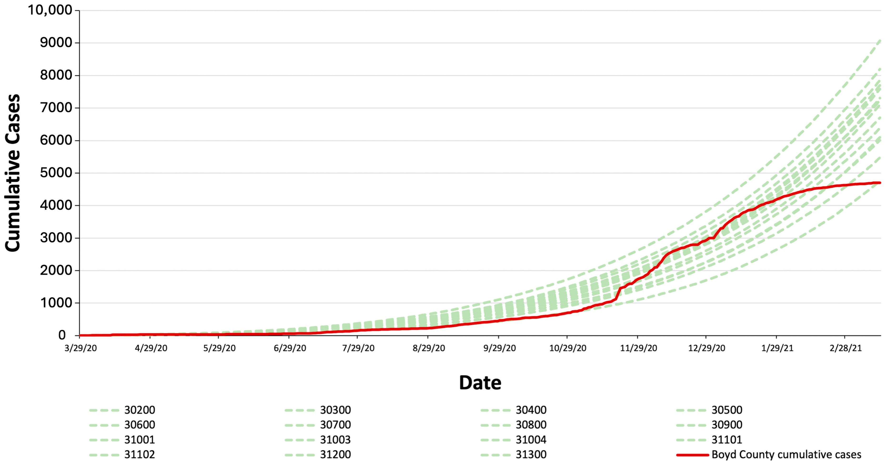
We conducted face validation and empirical validation at both micro- and macro-levels of the WBE model, as suggested by Wilensky and Rand [42] for ABM development. The face validation at the microlevel of the model involved examining whether the human agents behaved as intended, such as traveling and contacting others. The empirical validation at the microlevel involved examining the accuracy of the spatial distributions of sewered and non-sewered populations, the distributions of incubation periods for human agents, and values of relevant environmental parameters, to ensure they aligned with real-life scenarios. The face validation at the macro-level included two comparisons. First, we compared the emergent epidemic patterns in our model against the infection curve of an SEIR compartmental model to confirm that our model produced a typical epidemic pattern, i.e., a single-peaked infection curve followed by a decline as the susceptible population decreases. Second, since we relaxed two assumptions in the standard SEIR model by allowing for increased heterogeneity within populations in different geographical areas, we compared the emergent epidemic patterns in our model against the results from the previous studies with similar model settings [43] and confirmed that our model generated a similar epidemic pattern that showed a later and lower peak of the outbreak when the two assumptions were relaxed by integrating migration, social networks, and agent types and interactions into an agent-based epidemic model. We also calibrated the model, which is an empirical validation at the microlevel, based on the real-world epidemic data from the simulated county from 29 March 2020, to 15 March 2021, and SARS-CoV-2 seroprevalence. Table 2 gives the values of the variables used in the calibration. As shown in Figure 5, the simulated epidemic pattern closely matches the real-world data pattern from March 2020 to November 2020. Although the cumulative case numbers estimated by the model were higher than the actual data, we consider that they fell within an acceptable range because the real-world data came from clinical surveillance, which did not include undetected and asymptomatic cases. Estimates of the ratio of SARS-CoV-2 seroprevalence to COVID-19 case prevalence range from 2.6 to 3.5 [44], indicating an underreporting of actual clinical cases, further aligning our model predictions with clinical data from the early stage of the outbreak.
Table 2. Data Sets, Parameters, and variables used in the WBE model and the sources. The values of parameters are drawn from literature, and the values of variables are determined by the model calibration.
TypeNameValue for Model ValidationSource
DatasetCensus tract boundary data setversion 2021-22[27]
DatasetPopulation datareleased 2021[29]
DatasetCounty sewage infrastructure GIS data
ParameterSewage service coverage in the partially sewered tracts80%[22]
ParameterIncubation period6 days ±1 day[45]
ParameterDisease Period10 days ± 2 days[46]
ParameterInfectious period2 days + disease period[37]
ParameterQuarantine rate33%[44,47]
ParameterMortality0.9% (as of 29 April 2023)[48]
ParameterFamily contacts1–6 contactsCalculated based on population data
ParameterSchool contacts10–25 contactsCalculated based on population data
ParameterWorkplace contactsup to 13 contacts[31,33]
ParameterCommunity contactsup to 13 contacts[31,33]
Parameter% travelers within sewered or non-sewered zones25%[30]
ParameterVirus-shedding period21 days[49]
ParameterVirus load107.6 copies/mL[50]
ParameterFeces318 mL/day[51,52]
ParameterPercentage of infectious individuals shedding viruses43%[53]
ParameterWastewater Production19,043,452,054 mL/dayMeasured at the target wastewater treatment plant
VariableFamily transmission rate4%Calibrated against the county data
VariableSchool transmission rate0% School closure
VariableWorkplace transmission rate2% (weekdays); 0% (weekends)Calibrated against the county data
VariableCommunity transmission rate1.1% (weekdays); 1.2% (weekends)Calibrated against the county data
Variable%-travelers-across (between sewered and non-sewered zones)5% (weekdays); 10% (weekends)Calibrated against the county data
VariableVaccination rate 0%No vaccine available during the simulated time range
Figure 5. Comparison of simulated epidemic patterns when COVID-19 initiated in different census tracts (30 repetitions for each tract) and the real-world county epidemic pattern from 29 March 2020–15 March 2021.
Systems 13 01093 g005
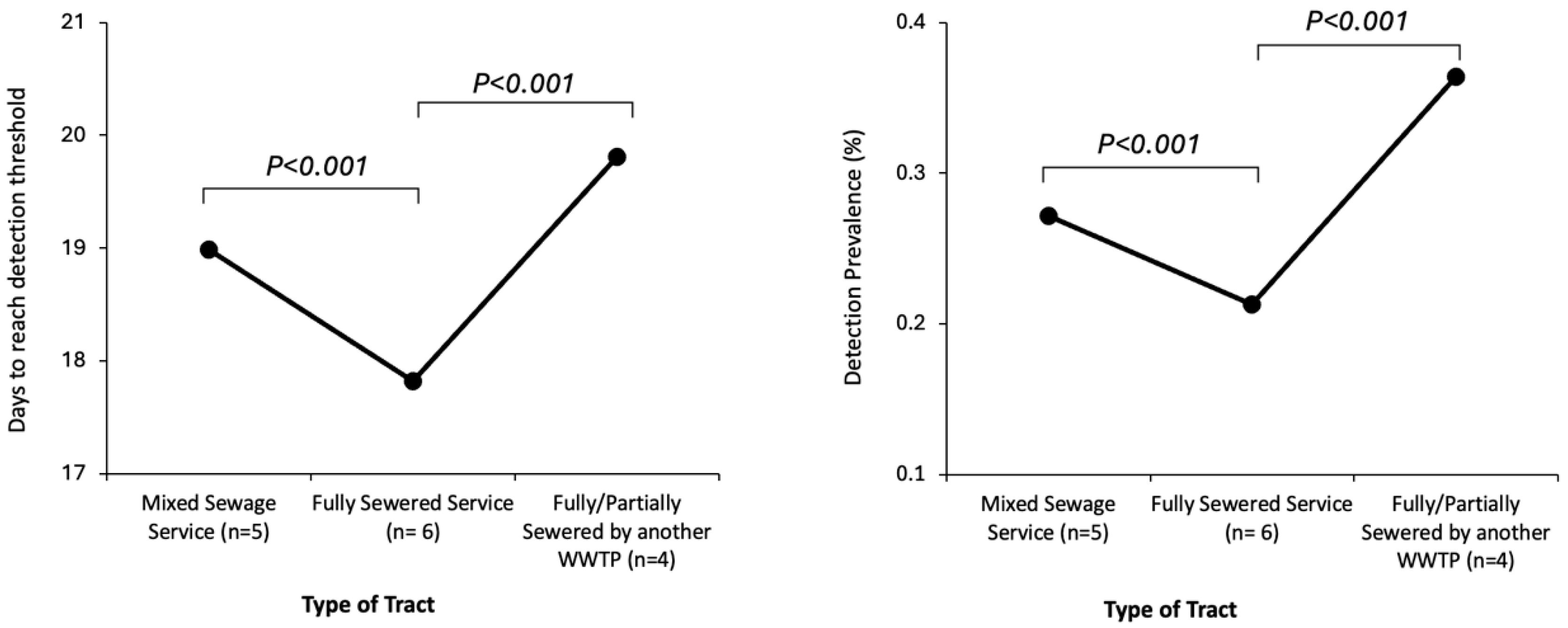
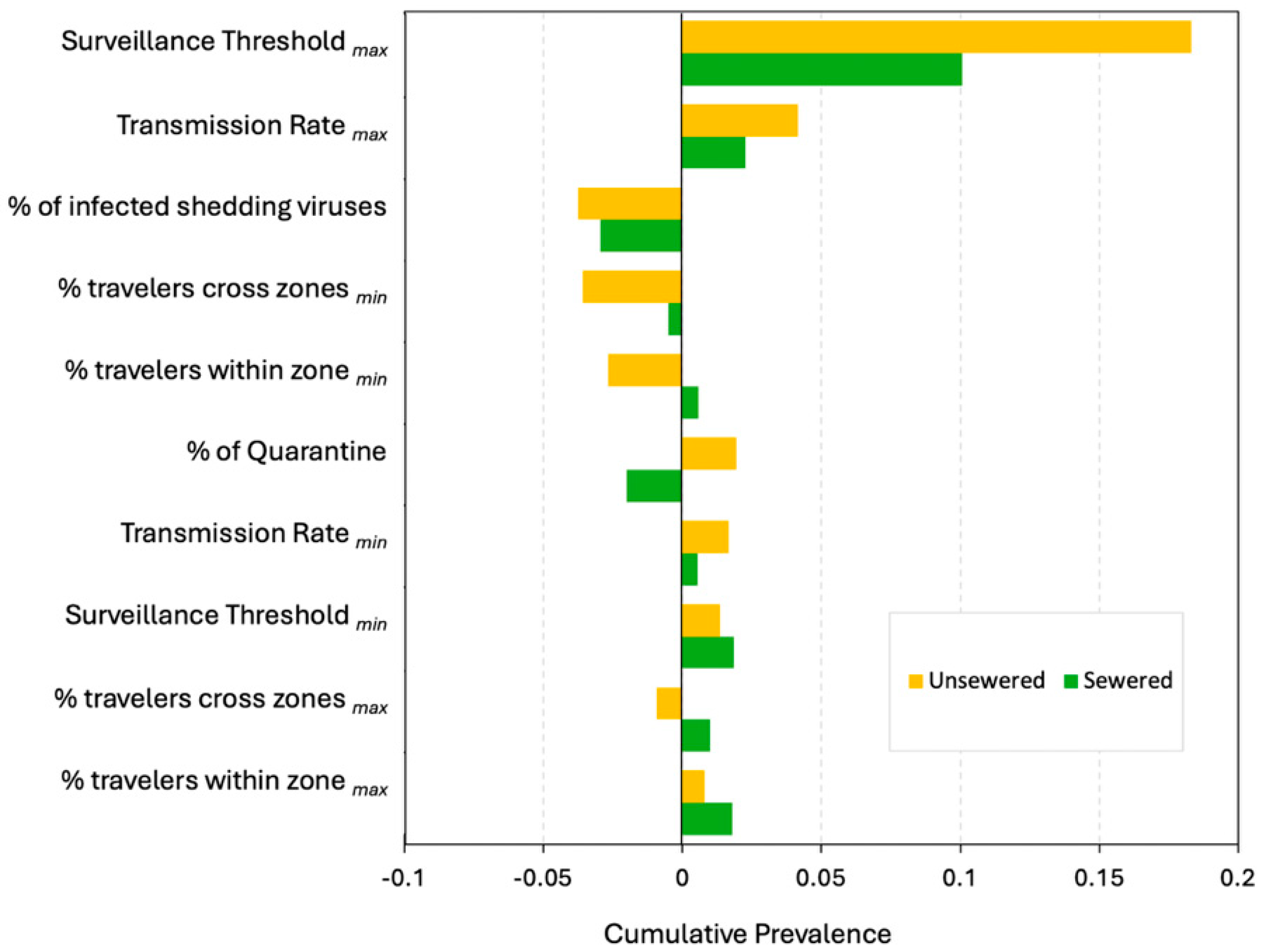
Both local and global sensitivity analyses were conducted during model verification (Appendix A). We conducted local sensitivity analysis using one-factor-at-a-time (OFAT) tests [54,55], a widely used local sensitivity analysis approach for agent-based modeling, and gained two insights. First, the analysis suggested that the detection timing and cumulative COVID-19 prevalence at the predefined WBE threshold significantly varied by tract type (i.e., mix of sewered and non-sewered, fully sewered, and fully or partially serviced by another wastewater treatment plant; Figure A1 in Appendix B). Second, the larger surveillance threshold, the higher disease transmission rate, the higher cross-zone travel rate, and the percentage of infectious individuals shedding viruses showed stronger influence on the cumulative COVID-19 prevalence for outbreaks originating in non-sewered zones (Figure A2 in Appendix C).
Next, based on these results and our research questions, we performed a global sensitivity analysis using a fractional factorial design [55,56] to examine the impacts and potential interactions of the transmission rate, surveillance threshold, disease transmission rate, and cross-zone travel rate on detection timing and cumulative COVID-19 prevalence for the five tracts with a mix of sewered and non-sewered areas. The global sensitivity analysis results are provided in Appendix D.

2.2. Scenarios Settings and Testing Procedure

After model validation and calibration, the WBE model was used to explore SARS-CoV-2 spread in the early epidemic stage within the simulated county in a series of 240 scenarios by combining the following four factors (1) theoretical basic reproduction numbers (R0), (2) epidemic initiated from sewered vs. non-sewered zones in five census tracts, (3) population mobility, and (4) WBE detection sensitivity.
Basic reproduction numbers (R0): As mentioned above, we selected the R0 of 4 and 8, because they were consistent with the R0 values of the Delta variant and the Omicron variant, as well as represent moderate to severe transmission situations. We calculated the transmission rate (TR) for the community network based on selected R0 (Equation (2)), as the network included the largest portion of the population. Once the TR of the community network was determined, the TRs for family, school, and workplace networks were adjusted based on the estimated daily contact duration. Specifically, we assumed 3 h of contact duration per day in the community, 6 h at school and work, and 12 h within households. Therefore, the TRs for the school and workplace networks were set at twice the community rate, while the TR for the family network was set at four times the community rate. In addition, the TRs for the school and workplace networks were set to zero on weekends, assuming no school or work occurred during those days (Table 3).
Initiation region of outbreaks: The sewage service status varied from fully sewered to partially sewered among the 15 census tracts in the county. Six tracts were fully sewered, and four tracts were not served by the wastewater treatment plant where the wastewater production data were collected. Therefore, the remaining five tracts were selected for our testing because they include both sewered and non-sewered populations, and their wastewater was processed by the target wastewater treatment plant. These five tracts comprised a total of 2363 unsewered adults, representing 70% of the county’s unsewered adult population.
Population mobility: In this study, we were interested in the epidemic patterns associated with the rates of cross-zone travel and tested the cross-zone travel rates at 0%, 2%, 4%, 6%, 8%, and 10%. The within-zone travel rate was held constant at 25%.
Wastewater surveillance detection sensitivity: In this study, we test two thresholds of wastewater SARS-CoV-2 detection, 10 gc/mL and 50 gc/mL, to closely match the lower and upper bounds of typical assay sensitivity [23].
A total of 240 simulation scenarios were established based on the above factors. Table 3 summarizes the variable value settings applied in these tests. Each scenario was run 30 times. In each trial, one exposed agent was introduced into the target census tract at the beginning. The model ran until seven days after the viral concentration in wastewater reached the predefined threshold, either 10 gc/mL or 50 gc/mL. To answer our research questions, we examined the number of days required to reach the WBE threshold, the corresponding disease prevalence, and the progression of disease prevalence over the subsequent week.

2.3. Data Analysis

We analyzed the data collected from a total of 7182 trials, after excluding 18 trials in which the outbreak failed to develop. The Kolmogorov–Smirnov tests [57] on the number of days required to reach the WBE threshold and the resulting disease prevalence were significant (p < 0.001), suggesting that these outputs were not normally distributed. Therefore, we performed Mann–Whitney U tests [58], a nonparametric statistical test, to compare results across different scenarios and used rank-biserial correlation (r) [59] and Eta squared (η2) to estimate the effect size of the tests [60].

3. Results

3.1. Impacts of WBE Detection Sensitivity, Sewage Service Status of the First SARS-CoV-2 Carrier, and Cross-Zone Travel Rate on the Number of Days Required for the Viral Concentration in the Aggregated Wastewater to Reach the WBE Detection Threshold

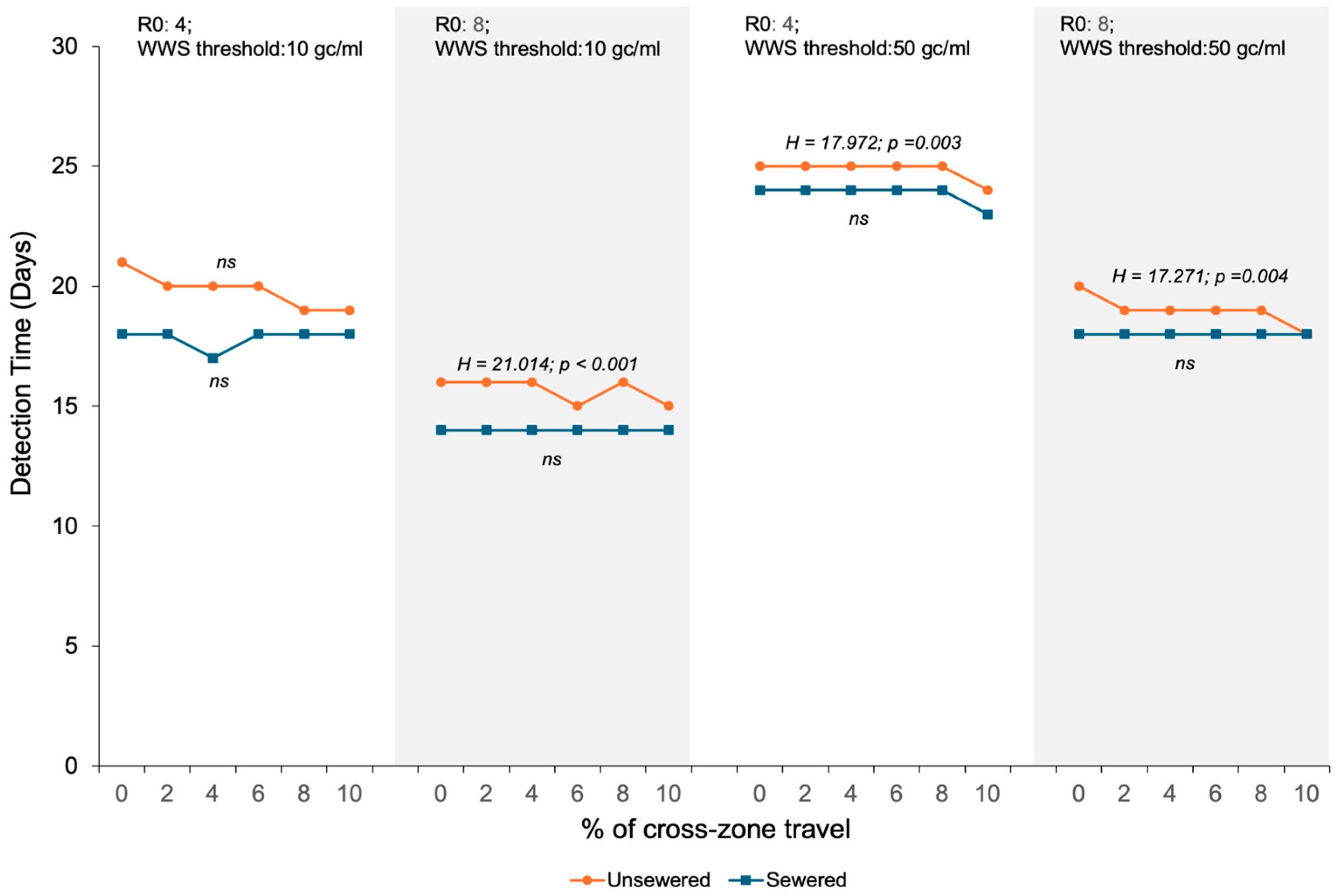
The WBE detection sensitivity threshold value significantly impacted the detection time with a large effect size (r: 0.58–0.72). With an R0 of 4, a detection threshold of 10 gc/mL resulted in SARS-CoV-2 RNA detection five days earlier for outbreaks originating in a non-sewered zone and six days earlier for outbreaks originating in a sewered zone than a threshold of 50 gc/mL; with an R0 of 8, a threshold of 10 gc/mL resulted in SARS-CoV-2 RNA detection three days earlier for outbreaks originating in a non-sewered zone and four days earlier for outbreaks originating in a sewered zone than the threshold of 50 gc/mL (Table 4).
The sewer service status of the first SARS-CoV-2 carrier also had a significant impact on the number of days required to reach the WBE detection threshold, with effect sizes ranging from small (r: 0.22–0.23) to medium (r: 0.32). With a WBE detection threshold of 10 gc/mL, it took 2 days longer for virus detection when an outbreak was initiated in non-sewered zones than in the sewered zones for R0 of 4 and 8. With a WBE detection threshold of 50 gc/mL, it took 1 day longer for virus detection when an outbreak initiated in non-sewered zones than in the sewered zones for both R0 of 4 and 8 (Table 4).
The detection time also decreased with increases in population cross-zone travel when the outbreak was initiated from the non-sewered zone. Significant changes were identified in three scenarios with a small effect size (η2: 0.014–0.018) (Figure 6). Pairwise comparisons revealed significant differences between the 0% and 10% cross-zone travel rates for an R0 of 4 (reduction of 1 day to detection), and between the 0% and 10% travel rates for an R0 of 8 (reduction of two days). There was no significant difference in detection time when the first SARS-CoV-2 carrier lived in a sewered zone (Figure 6).

3.2. Impacts of the WBE Detection Sensitivity, Sewage Service Status of the First SARS-CoV-2 Carrier, and Cross-Zone Travel Rate on the COVID-19 Prevalence When the Viral Concentration in the Pooled Wastewater Reaches the WBE Threshold

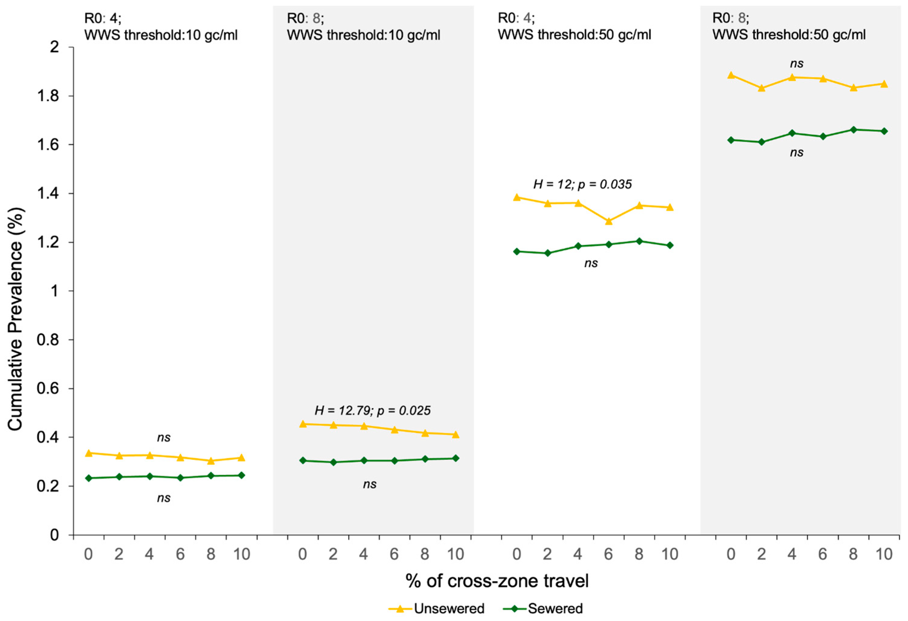
The WBE detection sensitivity significantly impacted COVID-19 prevalence when the WBE threshold was reached (hereafter referred to as threshold prevalence), with a large effect size (r: 0.87). With an R0 of 4, the 10 gc/mL threshold resulted in a 1.03% lower threshold prevalence for outbreaks originating in non-sewered zones than the 50 gc/mL threshold, equivalent to 498 fewer infections, given the total population of 48,447. Similarly, the threshold prevalence was 0.94% lower for outbreaks originating in sewered zones, equivalent to 457 fewer infections. With an R0 of 8, the 10 gc/mL threshold resulted in a 1.42% lower threshold prevalence for outbreaks originating in non-sewered zones and 1.33% lower threshold prevalence for outbreaks originating in sewered zones, corresponding to 689 and 646 fewer infections (Table 5).
The sewer service status of the first SARS-CoV-2 carrier had a significant impact on the threshold prevalence, with effect sizes ranging from medium (r: 0.29–0.34) to large (r: 0.52–0.53). Under the WBE threshold of 10 gc/mL, the threshold prevalence of the outbreaks initiated in non-sewered zones was 0.08% higher than that for the outbreaks initiated in sewered zones for the R0 of 4 and 0.13% higher for the R0 of 8, equivalent to 40 and 63 more infections. Under the WBE threshold of 50 gc/mL and with an R0 of 4, the threshold prevalence of the outbreaks initiated in non-sewered zones was 0.17% higher than that for the outbreaks initiated in sewered zones for the R0 of 4 and 0.22% higher for the R0 of 8, equivalent to 81 and 106 more infections (Table 5).
The threshold prevalence showed different trends along with the cross-zone travel rate in different zones (Figure 7). For the outbreaks originating in non-sewered zones, the threshold prevalence slightly decreased with increased cross-zone travel in all four scenarios. The decrease in threshold prevalence ranged from 0.019% to 0.043%. Significant changes were identified in two scenarios but with negligible effect sizes (η2: 0.008–0.009). Pairwise comparisons revealed that significant differences arose when the travel rate differed by 6% or more. For the outbreaks originating in sewered zones, the threshold prevalence slightly increased from 0.01% to 0.036%, with increased cross-zone travel in all four scenarios although the changes were not statistically significant.

3.3. COVID-19 Prevalence Trend over the Seven Days After the Wastewater Surveillance Threshold Is Reached in the Simulated County

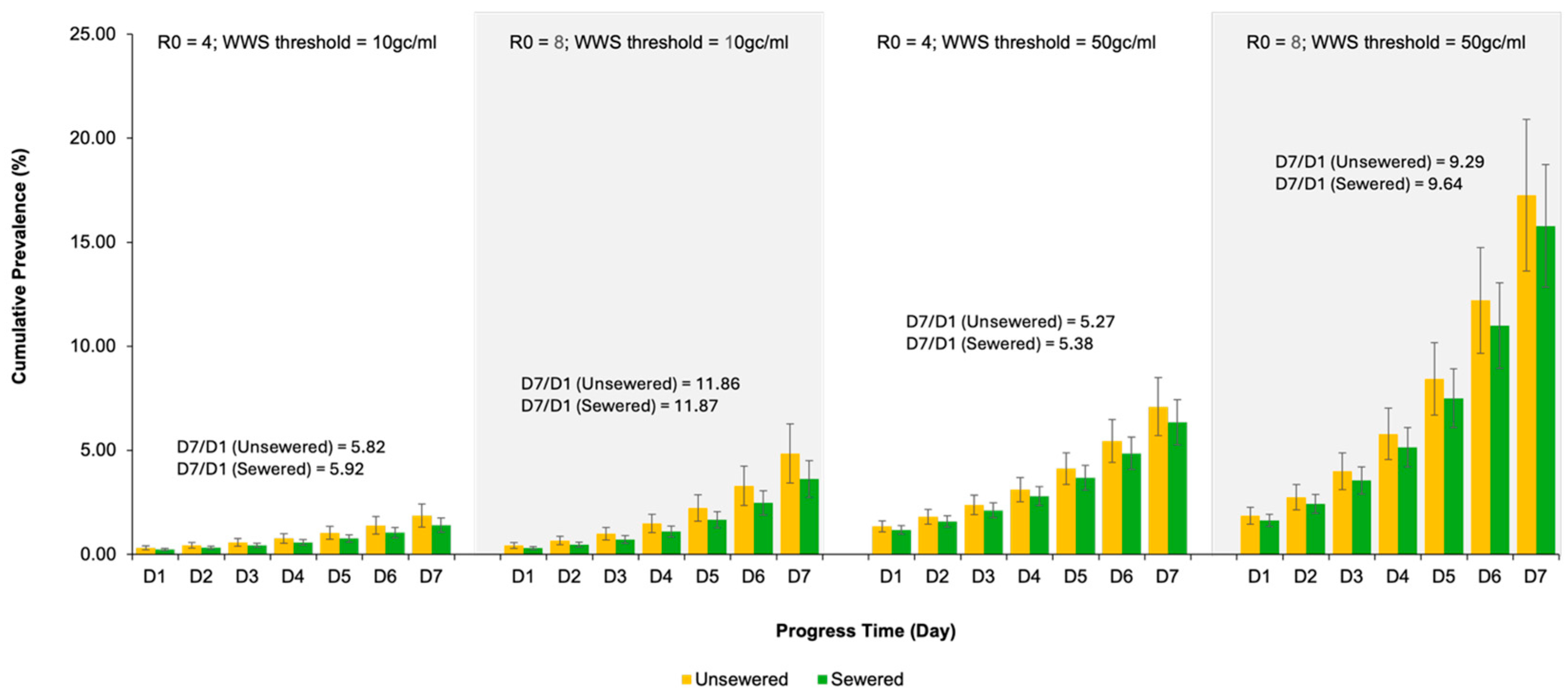
The WBE model indicates that the cumulative prevalence of COVID-19 drastically increased a week after the WBE threshold was reached. Taking the day when the WBE threshold was reached as Day 1, with an R0 of 4, the cumulative prevalence on Day 7 (hereafter referred to as Day-7 prevalence) in the simulated county was approximately 5.3–5.9 times higher than the threshold prevalence. With an R0 of 8, the Day-7 prevalence was about 9.3–11.9 times higher than the threshold prevalence (Figure 8).

4. Discussion

This study presents the development of a sophisticated agent-based WBE model that simulates COVID-19 transmission patterns in a region with a mixed wastewater infrastructure. Using the model, we evaluated the effectiveness of WBE in detecting a COVID-19 outbreak in the region when people are still mostly engaging in normal daily activities, with a low quarantine rate and no vaccination. This work is significant as (1) no similar model has been developed to explore the WBE of COVID-19 in an area with mixed WBE infrastructures, and (2) the modeling results provide comprehensive insights into how WBE detection sensitivity, sewage service status, and cross-zone community travel influence the effectiveness of WBE.
We found that the SARS-CoV-2 wastewater detection threshold strongly influences the timing of outbreak detection. Although it is intuitive that a more sensitive threshold leads to an earlier detection, our WBE model provides quantitative estimates of the performance of different detection thresholds. In our model, a threshold of 10 gc/mL results in substantially earlier detection (i.e., 5 to 6 days earlier for R0 of 4 and 3 to 4 days earlier for R0 of 8), more importantly, it identifies the outbreak while the cumulative number of infections is still relatively low (i.e., 0.24% to 0.32% for R0 of 4 and 0.31% to 0.44% for R0 of 8). These results are consistent with the work from Hart et al. [61] who reported that, assuming a threshold of 10 gc/mL, successful detection of SARS-CoV-2 by qRT PCR in fully homogenized wastewater requires a prevalence range from 0.00005% to 0.88%. In contrast, we observed that a threshold of 50 gc/mL not only detects an outbreak later but also captures it when the prevalence has reached 1.18% to 1.86% (i.e., 572 to 900 infections). This finding highlights the importance of selecting assay technologies with superior limits of detection.
The WBE model demonstrates that the sewer service status of the first SARS-CoV-2 carrier has a moderate influence on the outbreak detection timing in the tested settings. Before running the model, we hypothesized that there would be a delay in detecting the outbreaks initiated in the non-sewered zones because disease spread is likely to first occur through the networks of the carrier’s family and their neighboring community. This early local transmission will not be detected as the infected fecal waste does not enter the sewage systems. The model results supported our hypotheses and provided quantitative estimates of the delay. However, unlike the substantial changes in time and prevalence caused by different WBE detection thresholds, we observed only 1 to 2 days delay in detecting the outbreaks originating in the non-sewer zones and a moderately higher cumulative prevalence, ranging from 0.08% to 0.22% depending on the R0 and detection threshold. These increases are equivalent to 39 to 107 additional infections. This result suggests the need for tailored strategies for wastewater surveillance in non-sewered zones. Strategies that may lead to timely outbreak detection in non-sewered communities include: (1) facility-level wastewater surveillance at locations where unsewered community members spend time, such as local schools or regional employers/factories [62]; (2) testing of surface waters in communities where human waste enters the environment [63]; (3) use of emerging technologies to detect respiratory pathogens in the environment (e.g., air surveillance technologies) [64].
Cross-zone travel had a small effect on the time to detection and threshold prevalence as compared to changes in R0 or the wastewater testing sensitivity threshold because changes in detection time and threshold prevalence associated with the increases in cross-zone travel are small and often insignificant. However, we notice that the trends of the changes in threshold prevalence persist across all four scenarios, i.e., the threshold prevalence decreased with the increase in cross-zone travel for outbreaks initiated in non-sewered zone and it increased with the increase in cross-zone travel for outbreaks initiated in sewered zone (Figure 7). We may explain these trends using the WBE model rules. When the outbreak is initiated in the sewered zone, the infected fecal waste entered the sewage at the beginning of the outbreak. With the same R0, it takes a similar time to yield sufficient cases who shed viruses. When the cross-zone travel rate increases, more cases are likely to yield in non-sewered zones during the time, resulting in an increase in threshold prevalence. In contrast, when the outbreak is initiated in the non-sewered zone, without cross-zone travel or with only a low level of cross-zone travel, the chance of selecting the carrier on the first day is low, resulting in a longer detection time and higher threshold prevalence. When the cross-zone travel rate increases sufficiently, such as 8% or 10%, the unsewered carrier has a greater chance of traveling to the sewered zone and infecting the sewered population, resulting in earlier detection of the disease by WBE and a lower threshold prevalence. These trends are consistent with both the empirical observations and computer-simulated results that high population mobility and high R0 are associated with fast COVID-19 diffusion in a population [40,65,66]. The insignificant results could be because we only test the cross-zone travel rate up to 10% or the low non-sewered population. Given that only about 10% of the population is unsewered in the county, we kept the upper bound of the cross-zone travel rate at 10% to avoid an unrealistically high mobility level for community activities. In fact, the global sensitivity results indicated that the level of cross-zone travel rates tested in this study did not substantially affect the cumulative prevalence when the detection threshold was reached. However, the sewage service status and cross-zone travel exhibited a combined effect on cumulative prevalence. The workplace and school social networks’ contributions to disease transmission outweigh this level of cross-zone travel. In the future, we will test the setting with more trials, test higher cross-zone travel rates, or increase non-sewered population to gain more conclusive results.
This WBE model enables us to study disease transmission patterns based on the SARS-CoV-2 RNA detection threshold in the county’s wastewater treatment plant. Most wastewater treatment plants lack the capacity to test wastewater on-site and must rely on receiving test results from a centralized lab in a few days. We found that in an unvaccinated population similar to the modeled county, with a low quarantine rate (33%), the disease prevalence may increase by approximately 5- to 11-fold over a week. Notably, with an R0 of 8, which is consistent with the R0 of the Omicron variant, the disease prevalence may surge from 1.86% to 17.26% if the WBE threshold is 50 gc/mL and the outbreak is initiated in the non-sewered zones. Therefore, improving detection sensitivity and reducing sample-to-result turnaround time for local wastewater treatment plants and the non-sewered zone is critical and will contribute to early disease detection, thereby enhancing public health responses to COVID-19 and other similar infectious diseases.
Our WBE model has strengths and limitations. The main strengths lie in the integration of an SEIR epidemic model, detailed GIS sewage information of the county and sewage systems, and authentic data (i.e., county population demographics, population mobility, wastewater production, and clinic viral loads in feces) from an actual county to describe COVID-19 transmission patterns among a population of 48,447 inhabitants. We were able to validate and calibrate the model using the real-life epidemic data from the county. However, it is impossible to include all parameters or simulate all details of an outbreak. Simplifications and assumptions inevitably used in the model lead to several limitations. First, we do not include the virus degradation rate in wastewater or consider prolonged virus presence caused by biofilms in this model, which could either overestimate or underestimate the viral RNA concentration in wastewater. Second, we use feces as the only shedding source. Recent studies show other shedding routes, such as saliva, sputum, and urine, may also introduce SARS-CoV-2 RNA into wastewater [67,68]. Third, we use a single value for a few parameters in our tests, such as the values of virus shedding rate and quarantine rate. These simplifications were made due to limited real-world data and computational efficiency. In the future, a Monte Carlo approach could be used. Fourth, we assumed that agents only contributed sewage when at home; in reality, people living in unsewered houses likely use toilets at schools, workplaces, and other sewered sites. Thus, our model likely underestimated the viral concentration in the sewer system. Finally, our estimates of cross-zone travel would benefit from empirical data.
Our findings highlight the importance of basic reproduction numbers, sewer service status, community mobility patterns, and detection sensitivity when implementing WBE detection. By leveraging these insights, public health authorities can enhance preparedness and response strategies, ultimately improving community health outcomes. The model’s application to mixed infrastructural settings emphasizes the challenges and opportunities for WBE in such regions and suggests that tailored environmental surveillance strategies, such as those mentioned above, may better meet the specific needs of sewered and non-sewered areas, ensuring that early detection and intervention efforts are maximized. With this WBE model, we can estimate the effects of tailored interventions, such as mask-wearing, lockdowns, quarantines, or vaccinations. It can also be applied to investigate the epidemic patterns of other pathogens transmitted through the waterborne or fecal-oral routes by incorporating the relevant pathogenic matrices.

Author Contributions

Conceptualization, L.X., J.W.K., S.M.B. and A.S.; methodology, L.X. and J.G.; software, L.X.; validation, L.X., J.W.K., S.M.B. and J.G.; formal analysis, L.X.; GIS resources, J.G.; data curation, L.X.; writing—original draft preparation, L.X. and A.S.; writing—review and editing, J.W.K., S.M.B., A.S., E.L. and J.G.; visualization, L.X.; project administration, J.G. All authors have read and agreed to the published version of the manuscript.

Funding

This work was supported by the National Science Foundation (grants 2154934 and 2412446) and the NIH (U01 DA053903).

Data Availability Statement

Acknowledgments

We thank Alexus Rockward at the University of Kentucky for her assistance in identifying literature for model development.

Conflicts of Interest

The authors declare no conflicts of interest.

Appendix A

Table A1. Variable Settings for Sensitivity Analysis.
VariableFixedLocal SAGlobal SA
Transmission Rate (Community)2.5% (weekdays & weekend) 2.4%, 2.5%, 2.6% (weekdays & weekend)2.5%; 5%
4.8%, 5%, 5.3% (weekdays & weekend)
Transmission Rate (Family)10% (weekdays & weekend) 9.6%, 10%, 10.4% (weekdays & weekend) 5%; 20%
19.2%, 20%, 21.2% (weekdays & weekend)
Transmission Rate (School)5% (weekdays),
0% (weekend)
4.8%, 5%, 5.2% (weekdays),
0% (weekend)
5%;10%
9.6%, 10%, 10.4% (weekdays & weekend)
Transmission Rate (workplace)5% (weekdays),
0% (weekend)
4.8%, 5%, 5.2% (weekdays),
0% (weekend)
5%, 10%
9.6%, 10%, 10.4% (weekdays & weekend)
% travelers across zone10%Min: 0%, 0.5%, 1%0%, 2%, 4%, 6%, 8%, 10%
Max: 9.5%, 10%, 10.5%
% travelers within zone25%Min: 0%, 0.5%, 1%25%
Max: 23.75%, 25%, 26.25%
Quarantine rate33%31.35%, 33%, 34.65%33%
% of infected shedding virus43%40.85%, 43%, 45.15%43%
Viral RNA wastewater detection threshold≥10 gc/mLLower bound: ≥9.5 gc/mL, 10 gc/mL, 10.5 gc/mL≥10 gc/mL; ≥50 gc/mL
Upper bound: ≥47.5 gc/mL, 50 gc/mL, 52.5 gc/mL

Appendix B

Figure A1. Local sensitivity analysis on 15 tracts based on sewage service status. The detection time and cumulative prevalence differ significantly among tracts with three different types of sewage service status.
Systems 13 01093 g0a1

Appendix C

Figure A2. Results of the local sensitivity analysis performed on ten parameters of the wastewater-based epidemiological (WBE) model. The analysis quantifies the relative influence of each parameter on cumulative prevalence across both sewered and non-sewered regions. Findings indicate that the maximum surveillance threshold and the high transmission rate exert the greatest impact on cumulative prevalence.
Systems 13 01093 g0a2

Appendix D

Table A2. Summary of the statistical effects of four factors and their interactions on detection timing and corresponding cumulative prevalence. A check mark (✓) indicates a statistically significant effect, whereas a dash (–) denotes the absence of a statistically significant effect.
Days to Reach the Detection ThresholdCumulative Prevalence When Threshold Is Reached
Transmission Rate (TR)
Sewage service status (SSS)
% travelers across zone (T-across)
Surveillance Threshold (ST)
TR × SSS
TR × % T-across
TR × ST
SSS × T-across
SSS × ST
T-across × ST
TR × SSS × T-across
TR × SSS × ST
SSS × T-across × ST
TR × ST × T-across
TR × SSS × T-across × ST
R squared 0.5720.885

References

  1. Kilaru, P.; Hill, D.; Anderson, K.; Collins, M.B.; Green, H.; Kmush, B.L.; Larsen, D.A. Wastewater surveillance for infectious disease: A systematic review. Am. J. Epidemiol. 2023, 192, 305–322. [Google Scholar] [CrossRef]
  2. Larsen, D.A.; Green, H.; Collins, M.B.; Kmush, B.L. Wastewater monitoring, surveillance and epidemiology: A review of terminology for a common understanding. FEMS Microbes 2021, 2, xtab011. [Google Scholar] [CrossRef]
  3. Shah, S.; Gwee, S.X.W.; Ng, J.Q.X.; Lau, N.; Koh, J.; Pang, J. Wastewater surveillance to infer COVID-19 transmission: A systematic review. Sci. Total Environ. 2022, 804, 150060. [Google Scholar] [CrossRef]
  4. Johnson, S. The Ghost Map: The Story of London’s Most Terrifying Epidemic—And How It Changed Science, Cities, and the Modern World; Riverhead Books: New York, NY, USA, 2006. [Google Scholar]
  5. Sinclair, R.G.; Choi, C.Y.; Riley, M.R.; Gerba, C.P. Pathogen surveillance through monitoring of sewer systems. Adv. Appl. Microbiol. 2008, 65, 249. [Google Scholar]
  6. Asghar, H.; Diop, O.M.; Weldegebriel, G.; Malik, F.; Shetty, S.; El Bassioni, L.; Akande, A.O.; Al Maamoun, E.; Zaidi, S.; Adeniji, A.J.; et al. Environmental surveillance for polioviruses in the Global Polio Eradication Initiative. J. Infect. Dis. 2014, 210, S294–S303. [Google Scholar] [CrossRef]
  7. Wang, X.; Zheng, J.; Guo, L.; Yao, H.; Wang, L.; Xia, X.; Zhang, W. Fecal viral shedding in COVID-19 patients: Clinical significance, viral load dynamics and survival analysis. Virus Res. 2020, 289, 198147. [Google Scholar] [CrossRef] [PubMed]
  8. Ahmed, W.; Bertsch, P.M.; Bibby, K.; Haramoto, E.; Hewitt, J.; Huygens, F.; Gyawali, P.; Korajkic, A.; Riddell, S.; Sherchan, S.P.; et al. Decay of SARS-CoV-2 and surrogate murine hepatitis virus RNA in untreated wastewater to inform application in wastewater-based epidemiology. Environ. Res. 2020, 191, 110092. [Google Scholar] [CrossRef] [PubMed]
  9. Peccia, J.; Zulli, A.; Brackney, D.E.; Grubaugh, N.D.; Kaplan, E.H.; Casanovas-Massana, A.; Ko, A.I.; Malik, A.A.; Wang, D.; Wang, M.; et al. Measurement of SARS-CoV-2 RNA in wastewater tracks community infection dynamics. Nat. Biotechnol. 2020, 38, 1164–1167. [Google Scholar] [CrossRef] [PubMed]
  10. Larsen, D.A.; Wigginton, K.R. Tracking COVID-19 with wastewater. Nat. Biotechnol. 2020, 38, 1151–1153. [Google Scholar] [CrossRef]
  11. Cohen, A.; Vikesland, P.; Pruden, A.; Krometis, L.-A.; Lee, L.M.; Darling, A.; Yancey, M.; Helmick, M.; Singh, R.; Gonzalez, R.; et al. Making waves: The benefits and challenges of responsibly implementing wastewater-based surveillance for rural communities. Water Res. 2024, 250, 121095. [Google Scholar] [CrossRef]
  12. Jakariya, M.; Ahmed, F.; Islam, M.A.; Al Marzan, A.; Hasan, M.N.; Hossain, M.; Ahmed, T.; Hossain, A.; Reza, H.M.; Hossen, F.; et al. Wastewater-based epidemiological surveillance to monitor the prevalence of SARS-CoV-2 in developing countries with onsite sanitation facilities. Environ. Pollut. 2022, 311, 119679. [Google Scholar] [CrossRef]
  13. Ibrahim, S. A review of agent-based model simulation for COVID–19 spread. In Proceedings of the International Conference on Emerging Technologies and Intelligent Systems; Springer: Berlin/Heidelberg, Germany, 2022; pp. 585–602. [Google Scholar]
  14. Hunter, E.; Kelleher, J.D. Validating and Testing an Agent-Based Model for the Spread of COVID-19 in Ireland. Algorithms 2022, 15, 270. [Google Scholar] [CrossRef]
  15. Lorig, F.; Johansson, E.; Davidsson, P. Agent-based social simulation of the COVID-19 pandemic: A systematic review. JASSS J. Artif. Soc. Soc. Simul. 2021, 24, 5. [Google Scholar] [CrossRef]
  16. Xu, S.; Hsu, S.-C.; Du, E.; Song, L.; Lam, C.M.; Liu, X.; Zheng, C. Agent-Based Modeling in Water Science: From Macroscale to Microscale. ACS EST Water 2024, 4, 1206–1219. [Google Scholar] [CrossRef]
  17. Schuler, A.; Majed, N.; Bucci, V.; Hellweger, F.; Tu, Y.; Gu, A. Is the whole the sum of its parts? Agent-based modelling of wastewater treatment systems. Water Sci. Technol. 2011, 63, 1590–1598. [Google Scholar] [CrossRef]
  18. Fazli, M.; Sklar, S.; Porter, M.D.; French, B.A.; Shakeri, H. Wastewater-based epidemiological modeling for continuous surveillance of COVID–19 outbreak. In Proceedings of the 2021 IEEE International Conference on Big Data (Big Data), Orlando, FL, USA, 15–18 December 2021; pp. 4342–4349. [Google Scholar]
  19. DelaPaz-Ruíz, N.; Augustijn, P.; Farnaghi, M.; Abdulkareem, S.A.; Zurita-Milla, R. Integrating agent-based disease, mobility and wastewater models for the study of the spread of communicable diseases. Geospat. Health 2025, 20, 1326. [Google Scholar] [CrossRef]
  20. Bicker, J.; Tomza, N.; Wallrafen-Sam, K.; Schmid, N.; Hofmann, A.F.; Korf, S.; Schengen, A.; Javanmardi, J.; Wieser, A.; Kühn, M.J. Coupled Epidemiological and Wastewater Modeling at the Urban Scale: A Case Study for Munich. medRxiv 2025. [Google Scholar] [CrossRef]
  21. Schmid, N.; Bicker, J.; Hofmann, A.F.; Wallrafen-Sam, K.; Kerkmann, D.; Wieser, A.; Kühn, M.J.; Hasenauer, J. Integrative modeling of the spread of serious infectious diseases and corresponding wastewater dynamics. Epidemics 2025, 51, 100836. [Google Scholar] [CrossRef] [PubMed]
  22. United States Environmental Protection Agency. About Septic Systems. Available online: https://www.epa.gov/septic/about-septic-systems (accessed on 10 May 2023).
  23. Hewitt, J.; Trowsdale, S.; Armstrong, B.A.; Chapman, J.R.; Carter, K.M.; Croucher, D.M.; Trent, C.R.; Sim, R.E.; Gilpin, B.J. Sensitivity of wastewater-based epidemiology for detection of SARS-CoV-2 RNA in a low prevalence setting. Water Res. 2022, 211, 118032. [Google Scholar] [CrossRef]
  24. Wilensky, U. Center for connected learning and computer-based modeling. In NetLogo; Northwestern University: Evanston, IL, USA, 1999. [Google Scholar]
  25. Pilny, A.; Xiang, L.; Huber, C.; Silberman, W.; Goatley-Soan, S. The impact of contact tracing on the spread of COVID-19: An egocentric agent-based model. Connections 2021, 41, 25–46. [Google Scholar] [CrossRef]
  26. Grimm, V.; Railsback, S.F.; Vincenot, C.E.; Berger, U.; Gallagher, C.; DeAngelis, D.L.; Edmonds, B.; Ge, J.; Giske, J.; Groeneveld, J.; et al. The ODD protocol for describing agent-based and other simulation models: A second update to improve clarity, replication, and structural realism. J. Artif. Soc. Soc. Simul. 2020, 23, 7. [Google Scholar] [CrossRef]
  27. United States Census Bureau. Cartographic Boundary Files. Available online: https://catalog.data.gov/dataset/2024-cartographic-boundary-file-shp-census-tract-for-united-states-1-5000000 (accessed on 10 May 2023).
  28. QGIS.org. QGIS Geographic Information System; QGIS.org: Grüt, Switzerland, 2022. [Google Scholar]
  29. United States Census Bureau. Explore Census Data. Available online: https://www.usa.gov/agencies/u-s-census-bureau (accessed on 10 May 2023).
  30. Google. Community Mobility Reports; Google: Mountain View, CA, USA, 2022. [Google Scholar]
  31. Del Valle, S.Y.; Hyman, J.M.; Hethcote, H.W.; Eubank, S.G. Mixing patterns between age groups in social networks. Soc. Netw. 2007, 29, 539–554. [Google Scholar] [CrossRef]
  32. Mossong, J.; Hens, N.; Jit, M.; Beutels, P.; Auranen, K.; Mikolajczyk, R.; Massari, M.; Salmaso, S.; Tomba, G.S.; Wallinga, J.; et al. Social contacts and mixing patterns relevant to the spread of infectious diseases. PLoS Med. 2008, 5, e74. [Google Scholar] [CrossRef] [PubMed]
  33. Rothwell, J. Americans’ Social Contacts During the COVID-19 Pandemic. Available online: https://news.gallup.com/opinion/gallup/308444/americans-social-contacts-during-covid-pandemic.aspx (accessed on 15 June 2023).
  34. Phan, T.; Brozak, S.; Pell, B.; Gitter, A.; Xiao, A.; Mena, K.D.; Kuang, Y.; Wu, F. A simple SEIR-V model to estimate COVID-19 prevalence and predict SARS-CoV-2 transmission using wastewater-based surveillance data. Sci. Total Environ. 2023, 857, 159326. [Google Scholar] [CrossRef]
  35. McMahan, C.S.; Self, S.; Rennert, L.; Kalbaugh, C.; Kriebel, D.; Graves, D.; Colby, C.; Deaver, J.A.; Popat, S.C.; Karanfil, T.; et al. COVID-19 wastewater epidemiology: A model to estimate infected populations. Lancet Planet. Health 2021, 5, e874–e881. [Google Scholar] [CrossRef]
  36. Proverbio, D.; Kemp, F.; Magni, S.; Ogorzaly, L.; Cauchie, H.-M.; Gonçalves, J.; Skupin, A.; Aalto, A. Model-based assessment of COVID-19 epidemic dynamics by wastewater analysis. Sci. Total Environ. 2022, 827, 154235. [Google Scholar] [CrossRef] [PubMed]
  37. World Health Organization. Coronavirus Disease (COVID-19): How Is It Transmitted? Available online: https://www.who.int/news-room/questions-and-answers/item/coronavirus-disease-covid-19-how-is-it-transmitted (accessed on 10 May 2023).
  38. Jones, J.H. Notes on R0; Department of Anthropological Sciences, Stanford University: Stanford, CA, USA, 2007; Volume 323, pp. 1–19. [Google Scholar]
  39. Alimohamadi, Y.; Taghdir, M.; Sepandi, M. Estimate of the basic reproduction number for COVID-19: A systematic review and meta-analysis. J. Prev. Med. Public Health 2020, 53, 151–157. [Google Scholar] [CrossRef]
  40. Liu, Y.; Rocklöv, J. The reproductive number of the Delta variant of SARS-CoV-2 is far higher compared to the ancestral SARS-CoV-2 virus. J. Travel Med. 2021, 28, taab124. [Google Scholar] [CrossRef]
  41. Liu, Y.; Rocklöv, J. The effective reproductive number of the Omicron variant of SARS-CoV-2 is several times relative to Delta. J. Travel Med. 2022, 29, taac037. [Google Scholar] [CrossRef]
  42. Wilensky, U.; Rand, W. An Introduction to Agent-Based Modeling: Modeling Natural, Social, and Engineered Complex Systems with NetLogo; MIT Press: Cambridge, MA, USA, 2015. [Google Scholar]
  43. Hunter, E.; Kelleher, J.D. Understanding the assumptions of an SEIR compartmental model using agentization and a complexity hierarchy. J. Comput. Math. Data Sci. 2022, 4, 100056. [Google Scholar] [CrossRef]
  44. Wiegand, R.E.; Deng, Y.; Deng, X.; Lee, A.; Meyer, W.A.; Letovsky, S.; Charles, M.D.; Gundlapalli, A.V.; MacNeil, A.; Hall, A.J. Estimated SARS-CoV-2 antibody seroprevalence trends and relationship to reported case prevalence from a repeated, cross-sectional study in the 50 states and the District of Columbia, United States—October 25, 2020–February 26, 2022. Lancet Reg. Health–Am. 2023, 18, 100403. [Google Scholar] [CrossRef]
  45. Elias, C.; Sekri, A.; Leblanc, P.; Cucherat, M.; Vanhems, P. The incubation period of COVID-19: A meta-analysis. Int. J. Infect. Dis. 2021, 104, 708–710. [Google Scholar] [CrossRef]
  46. World Health Organization. Coronavirus Disease (COVID-19). Available online: https://www.who.int/health-topics/coronavirus#tab=tab_1 (accessed on 10 May 2023).
  47. Bergeri, I.; Whelan, M.G.; Ware, H.; Subissi, L.; Nardone, A.; Lewis, H.C.; Li, Z.; Ma, X.; Valenciano, M.; Cheng, B. Global SARS-CoV-2 seroprevalence from January 2020 to April 2022: A systematic review and meta-analysis of standardized population-based studies. PLoS Med. 2022, 19, e1004107. [Google Scholar] [CrossRef] [PubMed]
  48. Johns Hopkins University. Coronavirus Resource Center. Available online: https://coronavirus.jhu.edu/map.html (accessed on 10 May 2023).
  49. Jones, D.L.; Baluja, M.Q.; Graham, D.W.; Corbishley, A.; McDonald, J.E.; Malham, S.K.; Hillary, L.S.; Connor, T.R.; Gaze, W.H.; Moura, I.B. Shedding of SARS-CoV-2 in feces and urine and its potential role in person-to-person transmission and the environment-based spread of COVID-19. Sci. Total Environ. 2020, 749, 141364. [Google Scholar] [CrossRef]
  50. Foladori, P.; Cutrupi, F.; Segata, N.; Manara, S.; Pinto, F.; Malpei, F.; Bruni, L.; La Rosa, G. SARS-CoV-2 from faeces to wastewater treatment: What do we know? A review. Sci. Total Environ. 2020, 743, 140444. [Google Scholar] [CrossRef]
  51. NASA. NASA-STD-3001 Technical Brief: Body Waster Management: NASA Office of the Chief Health & Medical Officer (OCHMO). Available online: https://www.nasa.gov/ochmo/hsa-standards/ochmo-technical-briefs/ (accessed on 10 May 2023).
  52. Penn, R.; Ward, B.J.; Strande, L.; Maurer, M. Review of synthetic human faeces and faecal sludge for sanitation and wastewater research. Water Res. 2018, 132, 222–240. [Google Scholar] [CrossRef]
  53. Natarajan, A.; Zlitni, S.; Brooks, E.F.; Vance, S.E.; Dahlen, A.; Hedlin, H.; Park, R.M.; Han, A.; Schmidtke, D.T.; Verma, R. Gastrointestinal symptoms and fecal shedding of SARS-CoV-2 RNA suggest prolonged gastrointestinal infection. Med 2022, 3, 371–387.e9. [Google Scholar] [CrossRef]
  54. Ten Broeke, G.; Van Voorn, G.; Ligtenberg, A. Which sensitivity analysis method should I use for my agent-based model? J. Artif. Soc. Soc. Simul. 2016, 19, 5. [Google Scholar] [CrossRef]
  55. Railsback, S.F.; Grimm, V. Agent-Based and Individual-Based Modeling: A Practical Introduction; Princeton University Press: Princeton, NJ, USA, 2019. [Google Scholar]
  56. Borgonovo, E.; Pangallo, M.; Rivkin, J.; Rizzo, L.; Siggelkow, N. Sensitivity analysis of agent-based models: A new protocol. Comput. Math. Organ. Theory 2022, 28, 52–94. [Google Scholar] [CrossRef]
  57. Berger, V.W.; Zhou, Y. Kolmogorov–smirnov test: Overview. In Wiley Statsref: Statistics Reference Online; Wiley: Hoboken, NJ, USA, 2014. [Google Scholar]
  58. Mann, H.B.; Whitney, D.R. On a test of whether one of two random variables is stochastically larger than the other. Ann. Math. Stat. 1947, 18, 50–60. [Google Scholar] [CrossRef]
  59. Cureton, E.E. Rank-biserial correlation. Psychometrika 1956, 21, 287–290. [Google Scholar] [CrossRef]
  60. Levine, T.R.; Hullett, C.R. Eta squared, partial eta squared, and misreporting of effect size in communication research. Hum. Commun. Res. 2002, 28, 612–625. [Google Scholar] [CrossRef]
  61. Hart, O.E.; Halden, R.U. Computational analysis of SARS-CoV-2/COVID-19 surveillance by wastewater-based epidemiology locally and globally: Feasibility, economy, opportunities and challenges. Sci. Total Environ. 2020, 730, 138875. [Google Scholar] [CrossRef] [PubMed]
  62. Wannigama, D.L.; Amarasiri, M.; Hongsing, P.; Hurst, C.; Modchang, C.; Chadsuthi, S.; Anupong, S.; Phattharapornjaroen, P.; SM, A.H.R.; Fernandez, S.; et al. COVID-19 monitoring with sparse sampling of sewered and non-sewered wastewater in urban and rural communities. iScience 2023, 26, 107019. [Google Scholar] [CrossRef] [PubMed]
  63. Pocock, G. Application of wastewater-based surveillance to monitor SARS-CoV-2 prevalence in South African communities. Water Res. Comm. Pretoria. WRC Rep. No. TT 2020, 832, 20. [Google Scholar]
  64. Puthussery, J.V.; Ghumra, D.P.; McBrearty, K.R.; Doherty, B.M.; Sumlin, B.J.; Sarabandi, A.; Mandal, A.G.; Shetty, N.J.; Gardiner, W.D.; Magrecki, J.P.; et al. Real-time environmental surveillance of SARS-CoV-2 aerosols. Nat. Commun. 2023, 14, 3692. [Google Scholar] [CrossRef]
  65. Pullano, G.; Valdano, E.; Scarpa, N.; Rubrichi, S.; Colizza, V. Evaluating the effect of demographic factors, socioeconomic factors, and risk aversion on mobility during the COVID-19 epidemic in France under lockdown: A population-based study. Lancet Digit. Health 2020, 2, e638–e649. [Google Scholar] [CrossRef]
  66. Chagas, E.T.; Barros, P.H.; Cardoso-Pereira, I.; Ponte, I.V.; Ximenes, P.; Figueiredo, F.; Murai, F.; Couto da Silva, A.P.; Almeida, J.M.; Loureiro, A.A.; et al. Effects of population mobility on the COVID-19 spread in Brazil. PLoS ONE 2021, 16, e0260610. [Google Scholar] [CrossRef]
  67. Crank, K.; Chen, W.; Bivins, A.; Lowry, S.; Bibby, K. Contribution of SARS-CoV-2 RNA shedding routes to RNA loads in wastewater. Sci. Total Environ. 2022, 806, 150376. [Google Scholar] [CrossRef]
  68. Li, X.; Kulandaivelu, J.; Guo, Y.; Zhang, S.; Shi, J.; O’Brien, J.; Arora, S.; Kumar, M.; Sherchan, S.P.; Honda, R.; et al. SARS-CoV-2 shedding sources in wastewater and implications for wastewater-based epidemiology. J. Hazard. Mater. 2022, 432, 128667. [Google Scholar] [CrossRef]
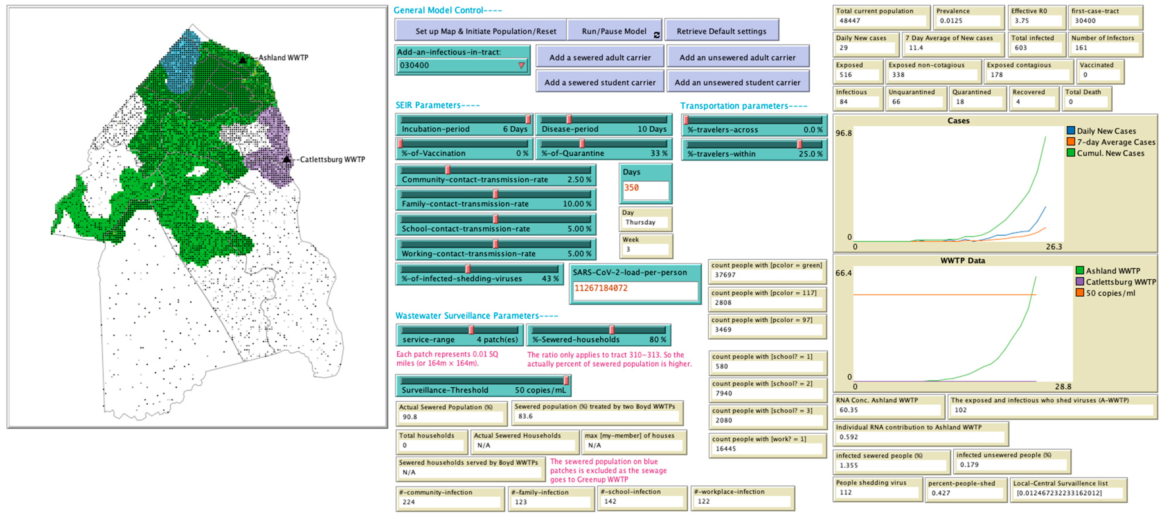
Figure 1. The WBE model interface. The left panel displays a spatial representation of the simulated county, divided into sewered (green, blue, purple) and non-sewered (white) zones. Human agents move and interact in these regions. The central panel presents the model control buttons and user-adjustable parameters. The right panel provides the real-time outputs, including case trajectories and wastewater detection results.
Systems 13 01093 g001
Figure 2. WBE model initiation.
Systems 13 01093 g002
Figure 3. People may travel within the sewered (green, blue, purple) or non-sewered (white) zone (a) and across sewered and non-sewered zones (b) for social community activities. This travel only affects the community network.
Systems 13 01093 g003
Figure 4. SEIR Compartmental Model.
Systems 13 01093 g004
Figure 6. Time to wastewater SARS-CoV-2 detection with varying levels of cross-zone travel, virus detection threshold, and sewer service status of the initial case. For outbreaks originating in non-sewered zones, the detection time slightly decreases along with the increase in the population cross-zone travel rate. Significant changes are identified in three scenarios with a small effect size (η2: 0.014–0.018). For outbreaks originating in sewered zones, no significant (ns) changes are observed in detection time.
Systems 13 01093 g006
Figure 7. For the outbreaks originating in non-sewered zones, the threshold prevalence slightly decreases along with the increase in population cross-zone travel rate. Significant changes are identified in two scenarios, but with a negligible size (η2: 0.008–0.009). For the outbreaks originating in sewered zones, the threshold prevalence slightly increases along with the increase in population cross-zone travel rate, although no significant (ns) difference is identified.
Systems 13 01093 g007
Figure 8. COVID-19 prevalence (M ± SD) upon reaching the WBE threshold and its progression over the subsequent week for outbreaks initiated in sewered and non-sewered zones under two WBE thresholds and basic reproduction numbers (R0) of 4 and 8. The relative fold increases in cumulative prevalence from Day 1 to Day 7 (i.e., D7/D1) are also shown.
Systems 13 01093 g008
Table 1. State variables for each human agent.
CategoryVariableVariable Specification
Geographic Locationtt-tract-IDHuman tract ID
home-x, home-yHuman home coordinates
Sewered?Human home sewage service status (True/False)
Disease TransmissionStates of diseasesusceptible, exposed (presymptomatic), infectious (symptomatic),
recovered
Measuresvaccinated, quarantine
Shed-pathogens?Does the person shed viruses?
Infected-by-meThe number of people the agent has infected
Infect-any?Has the agent infected any people? (True/False)
Social NetworkHousehold-idHousehold ID used to set up the family network
AgeAge in years
School?Does the person attend a school? (True/False)
class-IDA school attendee’s class ID
Work?Does the person work? (True/False)
Family-contactA person’s contacts at home
School-contactA school attendee’s contacts at school
Work-contactA worker’s contacts at the workplace
Non-community-contactA person’s combined contacts at home, school, and workplace.
Table 3. Variable Settings in the Early Detection Scenarios.
VariableR0 = 4R0 = 8
Transmission Rate (Community)2.5% (weekdays & weekend) 5% (weekdays & weekend)
Transmission Rate (Family)10% (weekdays & weekend) 20% (weekdays & weekend)
Transmission Rate (School)5% (weekdays),
0% (weekend)
10% (weekdays),
0% (weekend)
Transmission Rate (workplace)5% (weekdays),
0% (weekend)
10% (weekdays),
0% (weekend)
Effective contacts (Community)up to 13up to 13
Effective contacts (Family)1~61~6
Effective contacts (School)10~2410~24
Effective contacts (workplace)up to 13up to 13
% travelers across zone0%, 2%, 4%, 6%, 8%, 10% 0%, 2%, 4%, 6%, 8%, 10%
% travelers within zone25% 25%
Vaccination rate0%0%
Quarantine rate33%33%
Mean of Incubation period6 days ±16 days ± 1
Mean of disease period10 days±210 days ± 2
% of infected shedding virus43%43%
SARS-CoV-2 viral load per person per day11,267,184,072 copies/day11,267,184,072 copies/day
Viral RNA wastewater detection threshold≥10 gc/mL, ≥50 gc/mL≥10 gc/mL, ≥50 gc/mL
Table 4. Days needed to reach the WBE threshold for outbreaks originating in sewered and non-sewered zones under two detection thresholds and R0 of 4 and 8.
R0Sewer
Service
DaysMann–Whitney UEffect Size
WBE Threshold = 10 gc/mLWBE Threshold = 50 gc/mL
Median (IQR)Median (IQR)Zpr
4Non-sewered20 (18–22)25 (23–27)25.499<0.0010.60
Sewered18 (16–20)24 (22–25)29.942<0.0010.71
8Non-sewered16 (14–18)19 (18–21)24.676<0.0010.58
Sewered14 (13–16)18 (17–19)30.432<0.0010.72
Table 5. Cumulative disease prevalence upon the WBE threshold was reached for outbreaks originating in sewered and non-sewered zones under two surveillance thresholds and R0 of 4 and 8.
R0Sewer ServiceCumulative PrevalenceMann–Whitney UEffect Size
WBE Threshold = 10 gc/mLWBE Threshold = 50 gc/mL
M ± SD# of InfectionM ± SD# of InfectionsZpr
4Non-sewered0.32% ± 0.10%155 ± 481.35% ± 0.27%653 ± 12936.59<0.0010.87
Sewered0.24% ± 0.05%115 ± 271.18% ± 0.21%572 ± 10036.712<0.0010.87
8Non-sewered0.44% ± 0.14%211 ± 691.86% ± 0.41%900 ± 19736.697<0.0010.87
Sewered0.31% ± 0.07%148 ± 361.64% ± 0.30%794 ± 14436.732<0.0010.87
Disclaimer/Publisher’s Note: The statements, opinions and data contained in all publications are solely those of the individual author(s) and contributor(s) and not of MDPI and/or the editor(s). MDPI and/or the editor(s) disclaim responsibility for any injury to people or property resulting from any ideas, methods, instructions or products referred to in the content.