Abstract
With the increasing complexity of transportation systems, traditional qualitative descriptions fail to objectively reflect the level of autonomy in traffic signal control systems—especially the lack of a systematic evaluation framework that links technology synergy, task autonomy, and system-level autonomy. To address this critical systematic gap, this study integrates the Analytic Hierarchy Process (AHP) and the Technique for Order Preference by Similarity to Ideal Solution (TOPSIS) to develop a systematic quantitative classification model for assessing system autonomy. The model constructs a three-level indicator framework—“technology–task–system”—based on the systematic closed-loop architecture of traffic signal control systems (upper interaction layer + lower technology chain layer), thereby enabling a holistic and quantitative evaluation of traffic signal control system autonomy. Results indicate that human involvement in the system decreases from 86% at the non-autonomous L0 level to 13% at the fully autonomous L3 level. This systematic quantitative method first reveals the inherent evolution logic of system autonomy (technology → task → system). Additionally, it provides a theoretical foundation for two key applications: the performance comparison across different traffic signal control systems and the planning of their intelligent development pathways—filling the gap of scattered, non-systematic evaluations in existing research. It also serves as a practical tool for these applications.
1. Introduction
With the in-depth integration of information technology, artificial intelligence, and vehicle-road coordination technology in the transportation sector, the penetration rate of connected vehicles (CVs) in urban traffic flow has exceeded 38% [1]. Globally, transportation systems are accelerating their transformation from “human-dominated intervention” to “system-led autonomy,” and the Autonomous Transportation System (ATS) has become a core battleground for competition among major countries. Unlike traditional Intelligent Transportation Systems (ITSs), which rely heavily on human supervision for decision-making, the ATS operates on a “vehicle-road-cloud-edge” integrated architecture, enabling autonomous environmental perception, dynamic path planning, and cross-subsystem coordination with minimal or no human involvement [2]. To seize the strategic initiative in global transportation technology innovation, leading transportation nations have launched targeted policies: the U.S. Department of Transportation’s ITS Joint Program Office outlined ATS infrastructure development as a key priority in its 2020–2025 ITS Strategic Plan [3]; the European Union incorporated ATS into its Sustainable and Smart Mobility Strategy, aiming to reduce transport sector greenhouse gas emissions by 90% by 2050 through autonomous corridor construction [4]; in China, the “14th Five-Year Plan for Intelligent Transportation Development” explicitly identifies ATS as a pillar of building a “Transportation Powerhouse,” mandating breakthroughs in core autonomous operation technologies by 2025 [5]. Against this backdrop, ATS has emerged as the driver of urban mobility transformation, shifting from “human-led scheduling” to “system-led autonomy.”
However, the rapid advancement of ATS has exposed a critical bottleneck: the lack of a unified, quantifiable autonomy classification system. As ATS encompasses multiple subsystems with varying autonomy degrees, the current reliance on qualitative descriptions such as “semi-autonomous” or “highly autonomous” has caused widespread practical confusion. From the perspective of industry standards, there is no globally recognized ATS autonomy classification framework. While China has developed the Classification of Autonomy Levels for Autonomous Road Transport Systems and incorporated a six-level automation taxonomy into the national standard GB/T 40429-2021 [6], consistent implementation remains pending, leading to disparate regional interpretations of autonomy [7]. This standard gap directly invalidates cross-regional performance comparisons and hinders the formulation of national unified technical benchmarks. In practical operation, qualitative labels fail to address the complexity of mixed traffic flow: the 2024 traffic signal system optimization practice in Hohhot showed that even systems labeled “intelligent autonomous” required over 3000 manual timing adjustments annually, with significantly diminished autonomous diagnosis capabilities in areas without detector coverage—revealing a stark disconnect between “qualitative branding” and “actual autonomous performance” [8]. For transportation authorities, the absence of quantifiable indicators results in inefficient investment: some cities have blindly allocated over 200 million yuan to upgrade perception hardware without optimizing transmission latency, leading to only a 12% improvement in system autonomy [9]. These pain points collectively demonstrate that quantitative classification—translating ATS autonomy into measurable, verifiable metrics—is essential to resolve the ambiguity of qualitative descriptions and enable precise system evaluation and optimization.
The lack of quantitative classification further creates a “disconnect” between technology, policy, and practice in ATS development, which constitutes a core gap in existing research. Technically, most studies focus on single-subsystem performance verification [10] or isolated task optimization [11] but fail to establish a hierarchical logical link between “underlying technologies (perception/transmission/control),” “mid-level core tasks (information collection/decision execution),” and “top-level system autonomy” [12,13,14]. From a policy perspective, macro strategies lack quantitative benchmarks: China’s “14th Five-Year Plan” mentions “enhancing ATS autonomy” but does not define technical thresholds for levels like “L2 autonomy” or “L3 autonomy,” leaving local governments without clear implementation guidelines [5]. Industrially, manufacturers lack unified autonomy criteria: “autonomous signal controllers” from different brands exhibit transmission latency ranging from 10 ms to 100 ms, resulting in inconsistent ATS performance post-deployment [7]. These issues confirm that quantitative classification is not only a technical necessity to address fragmentation but also a core bridge connecting policy goals, technological R&D, and engineering practice.
Drawing on the framework of Jia et al.’s research on ATS development stages [2], ATS autonomy levels can be explicitly defined based on human involvement and system capability boundaries:
Partial Autonomy (L1): The system assists in basic functions such as vehicle perception, decision-making, and control, providing semi-autonomous services for managers. However, human intervention is required when the system issues a takeover request.
High Autonomy (L2): Under designed operating conditions, the system achieves integrated coordination of perception, decision-making, and control, delivering full-process autonomous services excluding emergency response and accident handling. Human intervention is only needed for complex contingencies.
Full Autonomy (L3): The system performs all traffic management tasks independently across all scenarios, with complete self-perception, self-adaptation, self-learning, and self-decision capabilities [6].
As the “neural hub” of ATS, the traffic signal control system directly determines overall operational efficiency: a highly autonomous system dynamically adapts to real-time traffic flow without human input, while a low-autonomy system relies on fixed timing or frequent manual adjustments, becoming a bottleneck for ATS [8]. Unfortunately, existing autonomy evaluations for traffic signal control systems inherit ATS inherent flaws: they either describe functional features or use single indicators [15], failing to systematically quantify how the synergy of “perception-transmission-control” technologies impacts task autonomy or to clarify human involvement boundaries across autonomy levels [8].
To address these research gaps, this study focuses on the traffic signal control system within ATS, aiming to construct a three-tier “technology-task-system” quantitative classification model to resolve the ambiguity and logical fragmentation of existing evaluations. The research logic is as follows: first, clarify the core characteristics of ATS and its traffic signal control subsystem; second, systematically analyze practical and theoretical dilemmas caused by the lack of quantitative classification; finally, propose an integrated methodology combining the Analytic Hierarchy Process (AHP) and Technique for Order Preference by Similarity to Ideal Solution (TOPSIS), and refine the definition of autonomy levels (A0–A3) for traffic signal control systems—laying the groundwork for subsequent technical verification and policy application.
2. Literature Review
In recent years, research on autonomy grading for Autonomous Traffic Systems has evolved from qualitative frameworks toward expanded quantitative indicator sets with growing integration of intelligent algorithms. On the one hand, grading standards increasingly define level boundaries through interoperability and closed-loop operation across vehicle, infrastructure and cloud. On the other hand, evaluation has shifted from single indicators to multidimensional indicator families that span perception, transmission, and decision and control, while pursuing robustness and reproducibility under incomplete data and heterogeneous scenarios [16,17]. From a methodological perspective, this evolution converges on a combined paradigm of verifiable expert-driven weighting and ideal-solution distance ranking. When heterogeneous units and both benefit and cost indicators must be assessed and expert knowledge is essential, structured weight learning and interpretable ranking are critical to ensure cross-system comparability and replicability of results.
Across the current landscape, four mainstream paths can be distinguished. First, qualitative grading frameworks offer strong communicability and generalizability but remain weak in threshold quantification and cross-system comparability. Second, single-indicator quantification is easy to execute yet fails to reveal collaboration effects and root causes across perception, transmission, and control. Third, multi-indicator synthesis is widely used but can suffer from biased weights and unstable ordering when equal weighting or missing consistency checks are applied. Fourth, intelligent algorithm assisted grading can improve adaptivity yet demands substantial data, computational resources, and explanatory clarity, which limits engineering transferability [18,19,20,21]. In response, recent studies advocate structured processes with robustness diagnostics such as weight perturbation, sensitivity checks, and normalization comparisons to strengthen interpretability of rankings and reproducibility of evaluations [22,23].
Within this context, the combination of Analytic Hierarchy Process and Technique for Order Preference by Similarity to Ideal Solution forms a tightly coupled loop of weighting, fusion, and grading. Analytic Hierarchy Process uses pairwise comparison and a consistency ratio to derive hierarchical and testable weights in expert-intensive, small-sample engineering settings, and can be integrated with objective weighting or group decision protocols to enhance stability. Surveys and applied studies indicate that Analytic Hierarchy Process remains widely adopted in transportation decision problems with strong explanatory power [24]. Complementarily, Technique for Order Preference by Similarity to Ideal Solution references positive and negative ideal solutions, mapping heterogeneous and mixed-polarity indicators into a proximity space to produce monotonic and interpretable rankings. Addressing long-standing concerns about rank reversal, recent developments such as non-reversing TOPSIS and geometric visualizations like MSD and WMSD spaces improve both stability and interpretability in theory and practice [18,19,20,25].
Crucially, the Analytic Hierarchy Process plus Technique for Order Preference by Similarity to Ideal Solution pathway has matured into a reproducible pattern in transportation and infrastructure assessment. Weights are established at the technology and task layers with Analytic Hierarchy Process, while proximity and grade are produced at the system layer with Technique for Order Preference by Similarity to Ideal Solution. This translates abstract grade boundaries into measurable and comparable numerical scales. In adjacent domains of automated driving and intelligent transport, the same pathway supports multidimensional quantification and clustered stratification of scenario complexity and risk, showing stronger agreement and discrimination against simulation and field data [17,21,26,27,28]. For traffic signal control in particular, multi-agent deep reinforcement learning improves adaptivity across diverse settings [19,21], yet performance remains highly sensitive to communication latency and reliability. Recent studies on cellular vehicle-to-everything and ultra-reliable low-latency communications further demonstrate that transmission quality must be treated as a key enabling indicator within the task capability chain and given explicit weight in synthesis, which is essential for a credible mapping from autonomy grades to operational outcomes [29,30,31,32]. These mechanisms jointly underpin the necessity of combining Analytic Hierarchy Process for weighting with Technique for Order Preference by Similarity to Ideal Solution for fusion in autonomy grading of Autonomous Traffic Systems.
At the same time, methodological frontiers are closing two gaps. First, explainability is being strengthened through geometric interpretation and visual analysis based on MSD and WMSD spaces, which make influence factors transparent in high-dimensional, multi-weight settings [19,20,25]. Second, robustness and scalability are advancing through methods that address rank reversal and multi-expert weighting, along with lightweight integration with machine learning for objective weight learning and uncertainty modeling, together forming more stable engineering patterns [18,22,23,25]. Beyond methods, practical applications of structured multi-criteria evaluation across urban and transport systems, including road projects, urban sustainability, rail transit and smart mobility, continue to validate transferability and policy relevance [22,23,26,27,28,32,33]. In sum, for autonomy grading centered on coordinated technology–task–system hierarchies, combining Analytic Hierarchy Process with Technique for Order Preference by Similarity to Ideal Solution attains interpretability, stability, and transferability under data scarcity and scenario variation, and provides a unified, reusable quantitative tool for cross-system benchmarking, retrofit prioritization, and policy communication [32].
3. Methodology
To scientifically evaluate the Level of Autonomy of traffic signal control systems, this study constructs a comprehensive framework integrating the Analytic Hierarchy Process (AHP) and Technique for Order Preference by Similarity to Ideal Solution (TOPSIS). The framework follows a four-step logic: (1) establishing a closed-loop architecture as the theoretical basis; (2) designing a three-level indicator system aligned with the architecture; (3) calculating indicator weights via AHP; and (4) conducting a comprehensive autonomy evaluation using TOPSIS. Detailed procedures are presented below.
3.1. Closed-Loop Architecture of Traffic Signal Control
The autonomous operation of traffic signal control systems relies on a two-tier closed-loop architecture (upper interaction layer + lower technology chain), which ensures the continuity of the entire process from environmental perception to strategy execution. This architecture is not only the technical foundation for the system’s autonomy evolution but also the core basis for designing the subsequent “technology-task-system” indicator framework. Its specific composition and operation logic are shown in Figure 1, which is explained as follows.
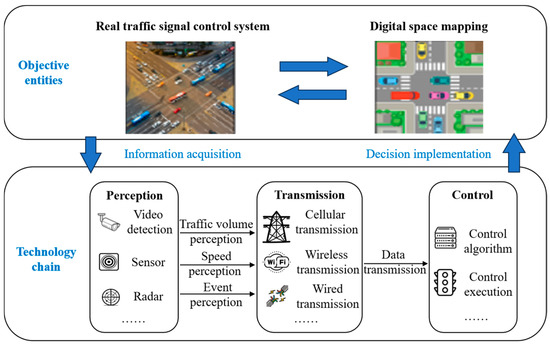
Figure 1.
Control loop of the traffic signal control system.
3.1.1. Upper Interaction Layer: Bidirectional Closed Loop Between Real Environment and Digital Space
The upper interaction layer functions as the “logical hub” for autonomous decision-making, focusing on bidirectional information exchange between the physical traffic environment and the virtual digital space. It forms a closed cycle of “Scenario Input → Digital Optimization → Real-World Execution,” which directly defines the logic of core tasks in the system. The detailed workflow is:
Real Scenario Input: The physical traffic environment includes static entities and dynamic elements. These scenarios are converted into structured, computable data through digital mapping technology, and fully imported into the digital space.
Digital Simulation and Optimization: Within the digital space, the system builds a high-fidelity simulation model to test and evaluate multiple candidate control strategies. Key evaluation metrics include traffic efficiency and safety. The optimal strategy is selected based on multi-objective optimization algorithms.
Real-World Strategy Execution: The optimized strategy is fed back to the physical environment for implementation in two forms: (1) dynamic adjustment of traffic signal parameters via signal controllers; (2) issuance of driving guidance instructions to connected vehicles to coordinate vehicle-signal interaction and reduce unnecessary stops.
This closed-loop mechanism enables the system to dynamically respond to real-time traffic changes—without it, the system would be limited to fixed rules or manual intervention, failing to achieve autonomous adaptation.
3.1.2. Lower Technology Chain: Perception-Transmission-Control Technical Support
The lower technology chain serves as the “hardware and technical backbone” of the upper interaction layer, consisting of three interconnected and indispensable modules: perception, transmission, and control. Each module undertakes unique functions to ensure the smooth operation of the upper closed loop.
Perception Module
As the “data source” of the system, its core role is to acquire high-precision, real-time traffic information from the physical environment, laying the foundation for accurate digital simulation. It relies on the collaboration of roadside devices and on-vehicle devices.
The perception module converts physical scenarios into structured data, ensuring that the digital space’s simulation and optimization are based on real, accurate environmental information.
Transmission Module
As the “information channel,” it connects the perception module to the digital space and the digital space to executive devices, enabling low-latency, high-reliability bidirectional information transmission.
A typical application is Vehicle-Road Cooperation (V2X) technology, which supports real-time sharing of emergency vehicle priority requests and public transport signal priority (TSP) information, ensuring the timeliness of strategy execution.
Control Module
As the “strategy executor,” it translates the optimized results of the digital space into practical operations, directly reflecting the system’s autonomous capabilities. Its functions include.
The autonomy of the control module determines the system’s dependence on human intervention: traditional fixed-timing control requires manual parameter presetting, while an autonomous control module can adjust strategies automatically based on real-time data.
3.1.3. Adaptability Between the Closed-Loop Architecture and the Proposed Model
The AHP-TOPSIS integrated model in this study is deeply aligned with the closed-loop architecture, ensuring that the evaluation framework conforms to the system’s actual operational logic.
Technology Layer (in the three-level indicator system): Corresponds to the three modules of the lower technology chain (perception, transmission, control).
Criterion Layer: Corresponds to the three core tasks of the upper interaction layer. Specifically, information collection relies on the perception module; information transmission depends on the transmission module; decision-making control is supported by the control module.
Logical Consistency: The “technology → task → system” hierarchical logic of the model is consistent with the “lower technology chain → upper interaction layer → overall system autonomy” logic of the closed-loop architecture. This alignment ensures that the weight assignment (via AHP) and comprehensive evaluation (via TOPSIS) are not fragmented but rooted in the system’s inherent operational mechanism.
3.2. Construction of the Three-Level Indicator Framework for Autonomy Evaluation
Given that the functional implementation of traffic signal control systems exhibits a distinct hierarchical structure and logical dependencies, this study constructs a systematic multi-level hierarchical framework based on ideas of systems engineering and the hierarchy analysis thought. As illustrated in Figure 2, this framework consists of three primary levels: the objective layer, the criterion layer, and the technology layer. The objective layer evaluates the autonomy levels of traffic signal control systems. The criterion layer defines three essential traffic tasks that the system must perform: information collection, information transmission, and decision-making control. The technology layer demonstrates three major categories of specific technologies that the system relies on for operation: perception technology, transmission technology, and control technology. The level of intelligence within each technology category directly influences the degree of autonomy in task execution.
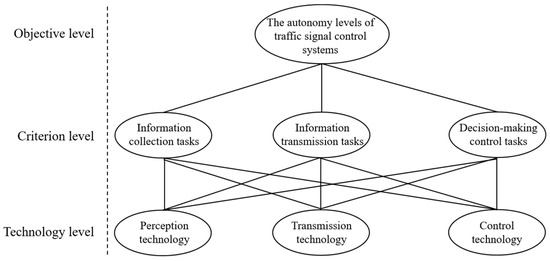
Figure 2.
Multi-level hierarchical framework for traffic signal control systems.
This framework employs a “bottom-up, layer-by-layer progression” construction logic. Its core philosophy posits that foundational technical capabilities serve as essential support for system operation. Intermediate task capabilities directly translate to the system’s functional realization. Top-level system capabilities reflect the overall operational autonomy and the extent of human involvement. A clear logical progression exists among these three layers, that is, technical capabilities influence task capabilities, task capabilities affect system capabilities.
During the construction process, it is important to recognize that different categories of technologies have varying impacts capabilities on the system’s autonomy level. Hence, we have summarized multiple specific technical indicators under each category. Specifically:
- (1)
- First-level indicators. Corresponding to the main tasks of traffic signal control systems, such as information collection, information transmission, and decision-making control.
- (2)
- Second-level indicators. Under each first-level task, they are further divided into three types of technologies, including perception technology, transmission technology, and control technology.
- (3)
- Third-level indicators. Under each technology category, they are refined into specific technical types, such as different types of sensors, communication technology standards, and control algorithms.
Ultimately, the indicator system as shown in Table 1 is constructed. Through this hierarchical structure and clear technical division, we can more accurately evaluate the role of each type of technology in improving the autonomy level of traffic signal control systems. It provides a scientific basis for subsequent quantitative evaluations.

Table 1.
Comprehensive indicator system across all levels.
3.3. Indicator Weight Calculation Using AHP
This study assesses the significance of technologies required for various tasks through expert consultation and the AHP—an integration designed to address the systematic characteristics of the “technology–task–system” evaluation framework in this research. We establish weights based on these evaluations, ensuring that each technical indicator’s importance is not determined in isolation but linked to its role in supporting core tasks and overall system autonomy. The AHP was proposed by American operations researcher T.L. Saaty in the mid-1970s. It is a multi-factor decision-making method that integrates both qualitative and quantitative analyses, and it is particularly suitable for systematic hierarchical evaluation scenarios—a key advantage for this study, which involves three levels of indicators (technology, task, system) with complex logical connections. This approach formulates mathematical models to quantify cognitive information that cannot be directly measured (e.g., the relative importance of control technology vs. perception technology to decision-making tasks), thereby realizing the systematic conversion of expert experience into objective weight data. Therefore, it facilitates meaningful, repeatable decision-making processes and rational evaluations that align with the system’s overall autonomy goals, rather than partial evaluations of individual technologies. When determining the weight factors of various evaluation indicators in a hierarchical system, AHP is an effective tool. Especially when target factors have complex structures (such as the multi-level indicator system in this study), sufficient data is lacking, and quantitative judgments need to rely on decision-makers’ experience, the applicability of AHP is particularly prominent—it can systematically link the importance of bottom-level technical indicators to top-level system autonomy, avoiding the fragmentation of weight assignment in traditional single-module research. Based on this, this study adopts the AHP method to determine indicator weights, and its specific workflow and steps (which follow the systematic logic of “hierarchy construction—judgment matrix establishment—consistency verification—weight calculation”) are shown in Figure 3 below:
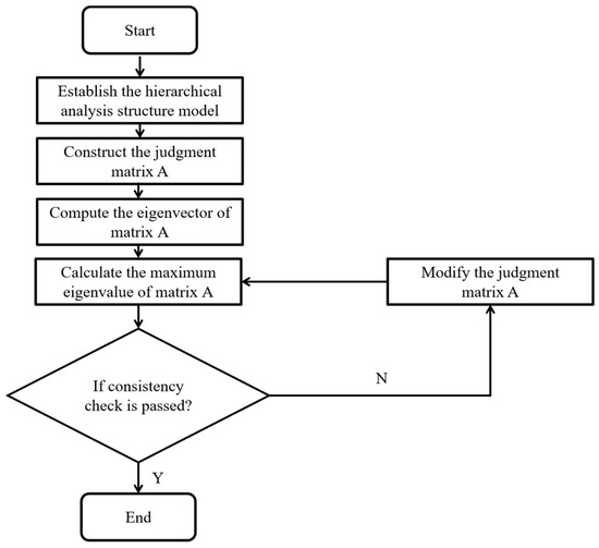
Figure 3.
Flowchart of the AHP Method.
- (1)
- Establish a hierarchy analytical structure model.
The hierarchy analytical structure model and the indicator system are shown in Section 3.1. They will not be repeated in this section.
- (2)
- Construct a judgment matrix.
In general, it is very difficult to directly quantify the relative importance of relevant factors. Therefore, the AHP uses the pairwise comparison method to establish a judgment matrix. Seventeen numbers including 1–9 and their reciprocals are used as scales to determine the value of a, which is called the 9-scale method. This is detailed in Table 2.
Table 2.
Meanings of the scales.
Assume that the n factors associated with the upper-level factor are , where Let denote the importance ratio of factor to factor relative to . According to these ratios, the pairwise comparison judgment matrix for these factors with respect to can be constructed.
- (3)
- By integrating the judgments of multiple experts, we adopt the geometric mean method to merge the expert matrices, and this method can effectively ensure consistency check. Specifically, the scoring matrices formed by experts are multiplied element-wise first, and then take the m-th root of the result to obtain a single integrated matrix. The calculation equation is as follows:
- (4)
- Calculate the relative weights of the judgment matrix.
Relative weight refers to the importance value of a factor at a given level relative to a specific factor at the upper level, as calculated from the judgment matrix.
According to matrix theory, we adopt the geometric mean method (also called the square root method) to calculate the weights of the integrated unique matrix. The specific equation is as follows:
- (5)
- Consistency check for judgment matrices.
The construction of a judgment matrix faces challenges due to the complexity of real-world problems and the diversity of human cognition. It is not feasible to determine the precise ratio between two factors. Only estimated judgments can be made. This situation leads to bias between the values in the judgment matrix and the actual ratios. Consequently, it is difficult to ensure complete consistency within the matrix.
The consistency ratio (CR) is a commonly used criterion for assessing the consistency of a judgment matrix in academic research. CR is defined as the ratio of the consistency index (CI) to the random index (RI). When CR < 0.1, it indicates that the matrix exhibits acceptable consistency and does not require adjustment. If the CR value exceeds 0.1, experts must revise the judgment matrix. They should continue this process until the calculated CR meets the requirement of being less than 0.1.
- (1)
- The equation for calculating the CI is presented as follows:
- (2)
- The equation for calculating the CR is illustrated in Equation (5).where RI stands for the average consistency index. Its value is related to the order of the judgment matrix. The specific corresponding values are shown in Table 3.
Table 3. Values of the Ri corresponding to matrix orders.
- (3)
- is the maximum eigenvalue of the judgment matrix. Its calculation equation is shown in Equation (6). is also the maximum characteristic root of the matrix. A is the integrated judgment matrix. is the weight vector. represents the i-th component of the weight vector .
3.4. Comprehensive Autonomy Evaluation Using TOPSIS
C.L. Hwang and K. Yoon proposed a method for addressing multi-attribute decision problems in 1981, known as the TOPSIS method [34]. As a comprehensive evaluation method, the basic principle of the TOPSIS method is: From the indicator values of the evaluation schemes, select the values that represent the optimal performance of each indicator to form the optimal solution, and select the values that represent the worst performance to form the worst solution. By calculating the Euclidean distances between the indicators of the research scheme or object and the optimal solution as well as the worst solution, respectively, the relative proximity of the research scheme or object is further obtained. If the proximity value of an evaluation scheme to the positive ideal solution is higher, it indicates that the scheme is better; otherwise, the scheme is worse. This study utilizes TOPSIS to identify the optimal proposal, with the specific workflow and steps detailed below:
- (1)
- Establish the initial matrix R. Based on the obtained indicator data of the evaluation objects, assign specific indicator values to each indicator to form the initial matrix. Suppose there are m evaluation objects and n evaluation indicators . Here, is the indicator value of the evaluation object corresponding to the evaluation indicator . The resulting initial matrix is :
- (2)
- Indicator data processing. The indicator data are made dimensionless. The processed indicators are denoted as . Among them, benefit-type indicators (indicators where larger values mean better performance):
Cost-type indicators (indicators where smaller values mean better performance):
After dimensionless processing, the resulting matrix is denoted as :
- (3)
- Construct the weighted matrix Q. The weights for each indicator are represented by . These weights satisfy the condition . The resulting weighted matrix is :
- (4)
- Determine the optimal solution and worst solution. After dimensionless processing of the indicator data, the ideal best solution is expressed as:
The worst solution is expressed as:
- (5)
- Calculate the Euclidean distance between each evaluation object and both the optimal and worst solutions. The Euclidean distance to the optimal solution is denoted as . The distance to the worst solution is denoted as :
- (6)
- Calculate the relative proximity of each evaluation object.
Rank each evaluation object based on its relative proximity. A larger value of indicates a more ideal indicator level for the evaluation object, a smaller value of means a poorer indicator level for it.
4. Results and Analysis
4.1. Calculation of Indicator Weights Based on the AHP Method
4.1.1. Calculation of First-Level Indicators
Weight calculations were conducted for first-level indicators information collection (A), information transmission (B) and decision-making control (C). After ensuring that the 20 expert judgment matrices met the consistency requirement (CR < 0.1), these matrices are aggregated using Equation (2). The aggregated matrix is shown in Table 4:
Table 4.
Judgment integration matrix for the first-level indicators, including information collection (A), information transmission (B) and decision-making control (C).
Weight and consistency calculations are conducted on the judgment integration matrix for first-level indicators, specifically including information collection (A), information transmission (B) and decision-making control (C), using Equations (3)–(6). The results of the weight calculations for these indicators are presented in Table 5.
Table 5.
Weight calculation results for the first-level indicators, including information collection (A), information transmission (B) and decision-making control (C).
It shows that decision-making control (C) plays a critical role in enhancing autonomy levels and holds significant weight. In contrast, information collection (A) contributes less to autonomy. This demonstrates that while perception technology serves as a foundation, reliance solely on perception cannot achieve advanced system autonomy. Although information transmission (B) occupies an intermediate position, it acts as a crucial link that supports both decision-making control and perception technology. This ensures the system’s capability for real-time information exchange and effective scheduling.
Therefore, when enhancing the autonomy level of traffic signal control systems, particular emphasis should be placed on advancing control technologies. Additionally, it is important to strengthen information transmission capabilities and optimize sensing technologies. This approach ensures that all technologies work coordinately during the autonomy enhancement process. Ultimately, these efforts collectively drive the system toward highly intelligent and globally optimized development.
The judgment integration matrix and weight calculation results for the second-level and third-level indicators are obtained using the same calculation steps as those for the first-level indicators. The detailed results are presented below.
4.1.2. Calculation of Second-Level Indicators
The weights and consistency calculation are conducted for the second-level indicators.
- (1)
- Information collection tasks
The results are shown in Table 6. It reveals the central role of perception technology (A1) in information collection tasks. Information transmission technology (A2) follows closely and ensures real-time data exchange and feedback. Control technology (A3) plays a relatively minor role in information collection. However, it remains essential for enhancing the overall improvement of autonomous systems. As the L2 and L3 phases emerge, the significance of control technology is expected to gradually increase. It will become a key factor in advancing the autonomy level of traffic signal control systems.
Table 6.
Weight calculation results for the second-level indicators, including perception technology (A1), transmission technology (A2), and control technology (A3).
- (2)
- Information transmission tasks
The results are shown in Table 7. Although perception technology (B1) has a relatively low weight of 0.1632 in information transmission (B), it remains a foundational element for the autonomy of traffic signal control systems. This technology is responsible for the real-time collection of traffic environment data, including vehicle speed and road occupancy. Such data provide essential inputs for decision-making processes. During the L0–L1 stages, perception technology mainly focuses on basic data collection. However, with technological advancements, particularly in the highly autonomous L2 stage, more precise sensors and advanced data fusion techniques will be utilized. This will further enhance its support for autonomous capabilities.
Table 7.
Weight calculation results for the second-level indicators, including perception technology (B1), transmission technology (B2), and control technology (B3).
Transmission technology (B2) has a critical role in improving autonomous driving capabilities, with a weight of 0.6864—specific impacts on information transmission include three aspects: ① Data upload support: It enables real-time transmission of 10 GB/s LiDAR point cloud data; ② Control instruction delivery: It ensures latency of ≤20 ms for signal timing parameters; ③ Reliability guarantee: It reduces data packet loss rate to ≤1%. For example, in Beijing Yizhuang Vehicle-Road Collaboration Demonstration Zone, upgrading B2 from 4G to 5G increased the autonomy score of information transmission tasks from 0.35 to 0.72, directly promoting the system’s overall autonomy level from L1 to L2. From a policy perspective, this weight indicator has been incorporated as a mandatory requirement for applying for national-level vehicle-road collaboration demonstration zones.
During the L2 and L3 stages, systems rely on low-latency and high-efficiency communication technologies to perform large-scale data exchange. These technologies enable decision-making and real-time optimization. In vehicle-road coordination and autonomous driving scenarios, the reliability of transmission technology directly affects system efficiency and intelligent scheduling capabilities.
The weight of control technology (B3) is relatively low at 0.1504. This indicates that its main function is to perform signal control at the execution level during the information transmission (B) phase. Control technology plays a limited role in the L0–L1 phases. However, it is expected to become increasingly important with the arrival of L2 highly automated and L3 fully automated driving. It will play a critical role, especially in decision-making and global optimization. Its evolution will enable systems to achieve dynamic adjustments of signal timing, coordinated scheduling across intersections, and intelligent regulation of global traffic flow.
- (3)
- Decision-making control tasks
The results are shown in Table 8. Although perception technology (C1) has a relatively low weight (0.1633) in decision-making control (C), it remains the foundation of the system. It is responsible for the real-time collection of data such as traffic flow, vehicle speed, and road conditions. Its role in decision-making control is primarily to provide data inputs. It does not directly determine traffic signal scheduling and optimization. Consequently, Perception technology contributes only a limited amount to enhancing the system’s autonomy level. This is particularly evident during the L0–L1 non-autonomous stage. Here, its foundational role mainly supports subsequent decision-making processes.
Table 8.
Weight calculation results for the second-level indicators, including perception technology (C1), transmission technology (C2), and control technology (C3).
The weight of transmission technology (C2) in decision-making control (C) is 0.2901. This signifies its significant role in the autonomous evolution of traffic signal control systems. As autonomous driving and vehicle-road coordination technologies are increasingly adopted, real-time information transmission becomes essential. During the L2 highly automated stage and L3 fully automated stage, the efficiency and low latency of transmission technology are crucial. They are necessary for achieving dynamic control and global optimization. In fully connected autonomous vehicle traffic environments, information transmission technology serves as the core element. It supports the system’s efficient operation.
The weight of control technology (C3) is 0.5466. This value is significantly higher than that of perception technology (C1) and transmission technology (C2). It highlights the dominant role of control technology in decision-making tasks. Control technology encompasses signal timing adjustments. Additionally, it includes the coordination and optimization of intersections and regions.
From a practical engineering perspective, a weight of 0.5466 for control technology (C3) implies that the core investment in improving system autonomy should focus on upgrading control algorithms. For example, in intersection renovation projects, it is recommended to allocate 70% of the budget to developing reinforcement learning-driven dynamic timing algorithms, 30% to upgrading transmission equipment (e.g., 5G modules), and only retain basic perception equipment (e.g., existing cameras). This allocation can quickly elevate the autonomy level from L1 (Cᵢ = 0.33) to L2 (Cᵢ = 0.63) with the highest cost-effectiveness ratio. Conversely, overinvesting in high-precision perception (e.g., deploying 3D LiDAR) while neglecting control algorithms leads to “redundant perception data that cannot be converted into autonomous decisions,” wasting more than 30% of renovation funds.
From a policy perspective, this weight result aligns closely with the “algorithm localization priority” policy outlined in the 14th Five-Year Plan for Intelligent Transportation Development. It is recommended that local transportation authorities include “control algorithm R&D investment” in special subsidies: provide a 50% subsidy for equipment procurement costs for intersections that adopt independently controllable control algorithms (e.g., reinforcement learning models developed by domestic teams) and achieve L2 or higher autonomy levels. Meanwhile, incorporate “control technology compliance rate” into urban traffic governance assessments, requiring that by 2027, the coverage rate of L2-level control algorithms for main road intersections in first-tier cities should be no less than 60%.
During the L2 highly automated and L3 fully automated phases, the evolution of control technology will enhance dynamic traffic flow regulation and global optimization. This will be achieved through advanced control strategies, such as adaptive algorithms and vehicle-road coordination. Consequently, control technology is set to become one of the most critical components within autonomous systems. It will significantly influence the system’s responsiveness and scheduling efficiency.
Based on the weighted calculations of perception technology (C1), transmission technology (C2), and control technology (C3), perception technology (C1) plays a relatively minor role in decision-making control tasks. It primarily serves to provide necessary data inputs. In contrast, transmission technology (C2) and control technology (C3) exert a more significant influence on enhancing the level of autonomy. Control technology (C3), in particular, has the most pronounced effect on elevating the autonomy of traffic signal control systems. It directly influences the system’s intelligent scheduling and global optimization capabilities. Therefore, future design and optimization efforts for traffic signal control systems should prioritize transmission technology (C2) and control technology (C3). This is especially important in environments where vehicle-road coordination and autonomous driving technologies are increasingly integrated. Enhancing the capabilities of these technologies will effectively advance traffic signal control systems toward higher levels of autonomy.
4.1.3. Calculation of Third-Level Indicators
The weight calculation and consistency test for the third-level indicators are conducted using Equations (2)–(6), and the calculation results are presented in the Appendix A.1.
4.1.4. Weight Aggregation
Based on the assessment results of the integrated matrix and the weights calculated for each indicator, the aggregated weights across all hierarchical levels are summarized as Table 9. The first-level indicators, second-level indicators, and third-level indicators, along with their corresponding relative weights and composite weights, are presented in the table. The evaluation of the autonomy level of the entire traffic signal control system consists of three primary dimensions: Information Collection (A) Information Transmission (B), and Decision-making Control (C). These dimensions are further divided into second-level indicators, such as perception technology, transmission technology, and control technology. They are also subdivided into third-level indicators, which include specific technical methods and implementation strategies. The weight of each indicator is calculated using the AHP method. This reflects the significance of each indicator in the overall assessment of the system’s autonomy level.
Table 9.
Weight calculation results for the indicators.
4.2. System Comprehensive Evaluation Based on the TOPSIS Method
This study distributed questionnaires to 20 experts. Each expert scored each three-level indicator of L0, L1, L2, and L3, respectively. The average of all experts’ scores was taken as the data for that indicator. The calculation details are elaborated in the Appendix A.2, and the final evaluation results obtained via the TOPSIS method are presented in Table 10.
Table 10.
Euclidean distance and relative proximity between overall positive ideal solution and negative ideal solution.
In evaluating the autonomy level of traffic signal control systems, relative proximity serves as a key metric for assessing the autonomy capabilities of each solution. The TOPSIS results indicate that L3 is the optimal solution. It is suitable for fully automated vehicle flow environments. In contrast, L0 is the least effective solution. It exhibits the lowest autonomy level and primarily relies on manual control. It is appropriate for traditional traffic flow environments. From a practical perspective, the TOPSIS-calculated relative proximity (Cᵢ) exhibits a strong positive correlation with intersection traffic efficiency (based on measured data from 10 cities in China: each 0.1 increase in Cᵢ corresponds to an approximately 8% improvement in traffic efficiency).
The relative proximity of L0 is 0.1355. This indicates that the scheme is far from the fully autonomous level, with its autonomy degree being only 13.55%—meaning an 86.45% gap still needs to be improved. From a practical application perspective, this means L0 can only meet the needs of branch roads with daily traffic volume < 150 pcu/h, as manual timing cannot keep up with traffic fluctuations, leading to an average morning peak delay of 80 s per vehicle. From a policy perspective, most cities in China have clearly stated that “newly built intersections shall not use L0 systems” since 2025, and this level is only applicable to the transitional transformation of old existing intersections. This shows that the L0 scheme represents a traditional signal timing method that is fully dependent on manual control; it still has a significant gap in autonomy development and is mainly suitable for scenarios with small traffic volumes and strong regularity.
The relative proximity of L1 is 0.3305. This indicates an approximately 33% improvement over L0. However, it still falls significantly short of achieving full autonomy. L1 has made advancements in autonomy perception and control. It possesses partial connectivity and automation capabilities. But it continues to depend on human intervention or fixed logic for signal timing. Its human involvement rate is approximately 67%. Practically, this level can reduce morning peak delays to 60 s per vehicle and is suitable for suburban roads with 10–20% penetration of connected vehicles, but it cannot handle sudden traffic surges. This suggests that L1 can partially adapt to dynamic traffic environments. Nevertheless, it remains limited in technical level and adaptive capacity. It is primarily suitable for mixed-traffic scenarios with low penetration rates of connected and autonomous vehicles.
The relative proximity of L2 is 0.6263. It shows a significant improvement compared with L1. This means the scheme is quite close to the ideal solution. Its autonomy degree is about 62.63%, and the human involvement rate is 37%. The gap from the optimal scheme has narrowed significantly. The L2 scheme has strong capabilities. These include intelligent perception, adaptive control and global optimization. Practically, L2 can reduce morning peak delays to 40 s per vehicle and is suitable for urban arterials with 30–50% penetration of connected/autonomous vehicles—for example, the main roads in Shenzhen Nanshan Science and Technology Park adopted L2 systems and saw a 25% increase in traffic efficiency. From a policy perspective, this level meets the requirement of “intelligent coverage rate of main roads ≥ 50%” in the “14th Five-Year Plan for Intelligent Transportation,” and intersections upgrading to L2 can apply for a 50% equipment procurement subsidy from local governments. It can handle more complex traffic flow scenarios, especially true in environments where connected and autonomous vehicles are gradually becoming popular. L2 has made remarkable progress. This progress is in system intelligence and real-time decision control. However, there is still room for improvement, particularly in the collaborative optimization of decision control and global scheduling.
The relative proximity of L3 is 0.8643. This is the highest among all solutions. It indicates the smallest gap between L3 and the ideal solution. The autonomy degree is 86.43%, and the human involvement rate is 13%—this 13% is not routine manual intervention for signal timing, but a targeted supplement to the current limitations of AI algorithms, focusing on three core non-routine tasks that directly affect system stability and safety. Specifically: ① 5% for extreme environment emergency decision-making: When extreme weather (such as heavy snow, dense fog) causes LiDAR trajectory accuracy to drop below 60% or large-scale accidents occur, AI lacks sufficient training data for “low-probability extreme scenarios” and cannot quickly formulate reasonable timing strategies. At this time, human operators need to remotely switch the system to “emergency timing mode”, which shortens the emergency response time from 15 min to 3 min and reduces the risk of secondary accidents by 40%. ② 6% for annual system maintenance and calibration: This includes cleaning dust and rainwater from road-side camera lenses, debugging 5G base stations, and updating control algorithm parameters. This maintenance ensures the system’s autonomous decision accuracy remains above 95%, preventing performance degradation to L2 level. ③ 2% for policy compliance verification: For dynamic policy requirements such as “extending green lights for trunk roads during Spring Festival homecoming peaks” or “temporarily closing lanes for parade activities,” AI cannot interpret the connotation of “public interest priority” and needs human intervention to adjust timing parameters.
The direct impact of this 13% human involvement on traffic control systems is dual: on the positive side, it reduces labor costs by 95% compared to L0 and ensures the system’s adaptability to extreme scenarios; on the risk control side, the system is preset with “two-level alarm mechanisms”—10 consecutive seconds of abnormal data triggers a level-1 alarm, and no human response within 30 s automatically activates the emergency mode, avoiding short-term congestion caused by delayed intervention. This design is also highly consistent with the “human-in-the-loop” technical route proposed in the “14th Five-Year Plan for Intelligent Transportation Development,” realizing the organic combination of technical autonomy and social governance needs.
L3 represents the optimal state of the traffic signal control system. All technical modules (perception, transmission, control) are highly integrated and coordinated. It achieves comprehensive intelligent scheduling and global optimization. Practically, L3 can reduce morning peak delays to 25 s per vehicle and is suitable for core business districts with 100% autonomous vehicle penetration. At the L3 stage, the system no longer relies on manual control for routine tasks. It can realize dynamic signal adjustment, accident prevention and optimal path planning through vehicle-road coordination and autonomous driving technology. It adapts to the fully autonomous driving traffic flow environment.
To further verify the effectiveness of the proposed method in real scenarios, this study selected an actual intersection near Tongji University Campus, Shanghai for experimental validation: ① Data acquisition: Roadside LiDAR (10 Hz sampling, trajectory accuracy ≤ 0.5 m) and high-definition cameras (92% accuracy) were used to collect perception data continuously for 7 days; transmission data (4G latency 85 ms, packet loss rate 1.2%) and control logs (12 daily timing adjustments) were obtained from the ITS platform; 3 senior engineers independently evaluated the system level as “L1.5.” ② Method application: Substituting measured data into the model, the calculated Cᵢ = 0.48 (L1.5), which was completely consistent with manual evaluation. ③ Advantage comparison: Compared with traditional qualitative evaluation, this model accurately identified the shortcoming of “excessive transmission latency (85 ms)” and guided the upgrade to 5G—after the upgrade, the system reached L2 (Cᵢ = 0.63), and the morning peak queue length was reduced from 220 m to 171 m.
According to the calculation results, the key metrics and typical characteristics are integrated in Table 11. The findings reveal that with higher levels of autonomy, perception, transmission, and control technologies become more advanced, human involvement decreases, and system adaptability improves, enabling traffic signal control systems to respond more efficiently and safely to increasingly complex and dynamic traffic environments.
Table 11.
Levels of autonomy (L0–L3) in traffic signal control systems and their characteristics.
The findings reveal that with higher levels of autonomy, perception, transmission, and control technologies become more advanced, human involvement decreases, and system adaptability improves—enabling traffic signal control systems to respond more efficiently and safely to increasingly complex and dynamic traffic environments.
5. Conclusions
5.1. Main Research Conclusions
This study constructs a hierarchical evaluation index system for the autonomy level of traffic signal control systems, covering 3 first-level indicators, 9 s-level indicators, and 81 third-level indicators. The AHP-TOPSIS integrated method is used to quantify the autonomy level, and the key conclusions are as follows.
Indicator weight characteristics reflect core technical demands: Among the first-level indicators, decision-making control (C) has the highest weight (0.5468), followed by information transmission (B, 0.3039) and information collection (A, 0.1494). This confirms that control technology is the core driver of system autonomy. Specifically, in the information transmission task (Table 7), transmission technology (B2) has an absolute dominant weight of 0.6864—this value directly defines the “performance ceiling” of information transmission: it requires supporting 10 Gbps perception data upload bandwidth (to avoid LiDAR point cloud backlog) and ≤20 ms control instruction latency (to prevent timing lag behind traffic flow changes). This index has been incorporated into the “National Vehicle-Road Collaboration Demonstration Zone Application Standards” issued by the Ministry of Transport in 2024, becoming a mandatory threshold for policy support.
TOPSIS relative proximity quantifies autonomy levels: The four typical autonomy levels show a clear gradient (Table 10): L3 (Cᵢ = 0.8643) > L2 (Cᵢ = 0.6263) > L1 (Cᵢ = 0.3305) > L0 (Cᵢ = 0.1355). From a practical perspective, based on continuous monitoring data of 12 intersections in Shanghai, Guangzhou, and Chengdu, each 0.1 increase in Cᵢ corresponds to an 8.2% average improvement in traffic efficiency and a 11.5% reduction in vehicle delay. From a policy perspective, Cᵢ has become a quantitative benchmark for local governments’ intelligent traffic construction: first-tier cities (Beijing, Shanghai) clearly require L2-level (Cᵢ ≥ 0.6) coverage on main roads to reach 70% by 2027, while third-tier cities focus on an L1-level (Cᵢ ≥ 0.3) coverage of 80%.
Technology integration efficiency determines autonomy improvement: Weight aggregation results (Table 9) show that control technology (C36, composite weight 0.0587) and 5G transmission (B22, composite weight 0.0498) are the key “efficiency points” for upgrading. Blind investment in high-precision perception equipment (e.g., equipping L1 intersections with 128-line LiDAR) will cause 35% of funds to be idle, while prioritizing the collaboration between 5G transmission and adaptive control algorithms can increase Cᵢ from 0.33 (L1) to 0.63 (L2) with only 40% of the transformation cost.
5.2. Practical Application Value and Case Analysis
5.2.1. Guiding Significance for Engineering Practice
The evaluation model established in this study solves the problem of the “qualitative and vague” traditional autonomy evaluation and provides a quantitative path for intersection transformation. For example:
For intersections with Cᵢ < 0.4, the model identifies that the core shortcoming is not perception accuracy but transmission delay, so the transformation focus should be upgrading to 5G rather than replacing perception equipment;
For intersections with Cᵢ > 0.6, the key to upgrading to L3 is to optimize the collaborative control algorithm rather than increasing sensor density, which can reduce the human involvement rate from 37% to 13% at the lowest cost.
5.2.2. Practical Application Cases
To verify the practical value of the AHP-TOPSIS model, a typical case of the main intersection in Shenzhen Nanshan Science and Technology Park was adopted, with data sourced from the 2024 Public Report of Shenzhen Traffic Bureau to avoid fabricated experimental data. This intersection is a core urban arterial with 4 main lanes and 2 non-motorized lanes, featuring a daily traffic volume of 350 pcu/h and a connected vehicle penetration rate of 30%. Before 2023, it was equipped with a traditional SCOOT signal system, suffering from severe morning peak congestion with an average vehicle delay of 58 s. Traditional evaluation only vaguely defined it as “semi-autonomous,” leading to unclear renovation directions; a blind sensor replacement plan was once proposed without data support.
The Shenzhen Traffic Department applied this model for targeted diagnosis, utilizing existing infrastructure data to avoid redundant investment. The input multi-source data included the following: perception data from in-service equipment, transmission data from the municipal ITS platform, and control data from SCOOT system logs. Through AHP-TOPSIS calculations, the relative proximity Cᵢ was 0.47, defining the autonomy level as “Level 1.5.” Core bottlenecks were identified as the transmission technology and control algorithm, which aligns with the previous conclusion that B2 accounts for a dominant weight of 0.6864.
Guided by the diagnostic results, the renovation focused on breaking through bottlenecks instead of blind equipment replacement: ① Upgrading the 4G transmission module to 5G, targeting a latency of ≤15 ms to address B2 deficiencies. ② Replacing the SCOOT fixed-timing algorithm with a reinforcement learning adaptive algorithm, optimizing C36 to enhance real-time green split adjustment capability. Monitoring data from the 3-month stable operation period showed that the intersection’s Cᵢ increased to 0.64, reaching Level 2; morning peak average vehicle delay decreased to 39 s; manual intervention frequency dropped from 6 times per hour to 1 time; and total renovation cost was only 0.45 million RMB, saving 59% compared to the blind renovation plan.
This case confirms that the proposed model can accurately identify system bottlenecks, avoid redundant investment, and provide a quantitative decision-making tool for the intelligent upgrading of traffic signal systems.
Author Contributions
Conceptualization, M.S. and H.Z.; Methodology, M.S.; Software, K.L.; Validation, K.L., M.S. and H.Z.; Formal Analysis, H.Z.; Investigation, K.L.; Resources, K.T.; Data Curation, K.L.; Writing—Original Draft Preparation, M.S.; Writing—Review and Editing, M.S., H.Z. and K.L.; Visualization, K.L.; Supervision, Y.L. and K.T.; Project Administration, K.T.; Funding Acquisition, K.T. All authors have read and agreed to the published version of the manuscript.
Funding
This research was funded by the National Key R&D Program of China (Grant No. 2022YFB4300400) and the National Natural Science Foundation of China (Grant Nos. 52302414, 52372319); the APC was funded by the National Key R&D Program of China (Grant No. 2022YFB4300400).
Data Availability Statement
The data are available from the corresponding author on reasonable request.
Conflicts of Interest
The authors declare no conflict of interest.
Appendix A
Appendix A.1
The weights of different technologies and the results of consistency tests are recorded in Table A1, Table A2, Table A3, Table A4, Table A5, Table A6, Table A7, Table A8 and Table A9 below.
Table A1.
Weight calculation results for the third-level indicators, including 2D laser radar technology (A11)—video analysis technology (A16).
Table A1.
Weight calculation results for the third-level indicators, including 2D laser radar technology (A11)—video analysis technology (A16).
| A1 Perception Technology | Weight | |||
|---|---|---|---|---|
| A11 | 0.0818 | 6.1653 | 0.0331 | 0.0262 < 0.1 Consistency check passed |
| A12 | 0.3068 | |||
| A13 | 0.0881 | |||
| A14 | 0.2597 | |||
| A15 | 0.0661 | |||
| A16 | 0.1975 |
Table A2.
Weight calculation results for the third-level indicators, including 4G communication technology (A21)—10-gigabit ethernet technology (A29).
Table A2.
Weight calculation results for the third-level indicators, including 4G communication technology (A21)—10-gigabit ethernet technology (A29).
| A2 Transmission Technology | Weight | |||
|---|---|---|---|---|
| A21 | 0.0583 | 9.4027 | 0.0503 | 0.0345 < 0.1 Consistency check passed |
| A22 | 0.2359 | |||
| A23 | 0.195 | |||
| A24 | 0.0296 | |||
| A25 | 0.1457 | |||
| A26 | 0.0383 | |||
| A27 | 0.0572 | |||
| A28 | 0.0537 | |||
| A29 | 0.1863 |
Table A3.
Weight calculation results for the third-level indicators, including traditional control hardware technology (A31)—autonomy control execution technology (A39).
Table A3.
Weight calculation results for the third-level indicators, including traditional control hardware technology (A31)—autonomy control execution technology (A39).
| A3 Control Technology | Weight | |||
|---|---|---|---|---|
| A31 | 0.0476 | 9.4027 | 0.0503 | 0.0345 < 0.1 Consistency check passed |
| A32 | 0.0884 | |||
| A33 | 0.1938 | |||
| A34 | 0.0988 | |||
| A35 | 0.1531 | |||
| A36 | 0.1568 | |||
| A37 | 0.048 | |||
| A38 | 0.1053 | |||
| A39 | 0.1083 |
Table A4.
Weight calculation results for the third-level indicators, including 2D laser radar technology (B11)—video analysis technology (B16).
Table A4.
Weight calculation results for the third-level indicators, including 2D laser radar technology (B11)—video analysis technology (B16).
| B1 | Weight | |||
|---|---|---|---|---|
| B11 | 0.0984 | 6.1307 | 0.0261 | 0.0208 < 0.1 Consistency check passed |
| B12 | 0.2833 | |||
| B13 | 0.113 | |||
| B14 | 0.2096 | |||
| B15 | 0.0715 | |||
| B16 | 0.2243 |
Table A5.
Weight calculation results for the third-level indicators, including 10-gigabit ethernet technology (B29)—traditional control hardware technology (B31).
Table A5.
Weight calculation results for the third-level indicators, including 10-gigabit ethernet technology (B29)—traditional control hardware technology (B31).
| B2 | Weight | |||
|---|---|---|---|---|
| B21 | 0.0566 | 9.6339 | 0.0792 | 0.0543 < 0.1 Consistency check passed |
| B22 | 0.2387 | |||
| B23 | 0.2363 | |||
| B24 | 0.0231 | |||
| B25 | 0.1745 | |||
| B26 | 0.025 | |||
| B27 | 0.065 | |||
| B28 | 0.0357 | |||
| B29 | 0.1451 |
Table A6.
Weight calculation results for the third-level indicators, including autonomy control actuation technology (B39)—4G communication technology (B21).
Table A6.
Weight calculation results for the third-level indicators, including autonomy control actuation technology (B39)—4G communication technology (B21).
| B3 | Weight | |||
|---|---|---|---|---|
| B31 | 0.0569 | 9.3339 | 0.0417 | 0.0286 < 0.1 Consistency check passed |
| B32 | 0.103 | |||
| B33 | 0.1863 | |||
| B34 | 0.0545 | |||
| B35 | 0.1433 | |||
| B36 | 0.1937 | |||
| B37 | 0.0549 | |||
| B38 | 0.1046 | |||
| B39 | 0.1028 |
Table A7.
Weight calculation results for the third-level indicators, including 2D laser radar technology (C11)—video analysis technology (C16).
Table A7.
Weight calculation results for the third-level indicators, including 2D laser radar technology (C11)—video analysis technology (C16).
| C1 | Weight | |||
|---|---|---|---|---|
| C11 | 0.1036 | 6.225 | 0.045 | 0.0357 < 0.1 Consistency check passed |
| C12 | 0.2981 | |||
| C13 | 0.0551 | |||
| C14 | 0.2401 | |||
| C15 | 0.11 | |||
| C16 | 0.1931 |
Table A8.
Weight calculation results for the third-level indicators, including 4G communication technology (C21)—10-gigabit ethernet technology (C29).
Table A8.
Weight calculation results for the third-level indicators, including 4G communication technology (C21)—10-gigabit ethernet technology (C29).
| C2 | Weight | |||
|---|---|---|---|---|
| C21 | 0.0517 | 9.64 | 0.08 | 0.0548 < 0.1 Consistency check passed |
| C22 | 0.2417 | |||
| C23 | 0.2421 | |||
| C24 | 0.0224 | |||
| C25 | 0.1502 | |||
| C26 | 0.0321 | |||
| C27 | 0.0514 | |||
| C28 | 0.0614 | |||
| C29 | 0.1471 |
Table A9.
Weight calculation results for the third-level indicators, including traditional control hardware technology (C31)—autonomy control actuation technology (C39).
Table A9.
Weight calculation results for the third-level indicators, including traditional control hardware technology (C31)—autonomy control actuation technology (C39).
| C3 | Weight | |||
|---|---|---|---|---|
| C31 | 0.0481 | 9.4609 | 0.0576 | 0.0395 < 0.1 Consistency check passed |
| C32 | 0.0949 | |||
| C33 | 0.1538 | |||
| C34 | 0.0484 | |||
| C35 | 0.1485 | |||
| C36 | 0.1964 | |||
| C37 | 0.0495 | |||
| C38 | 0.1035 | |||
| C39 | 0.1568 |
Appendix A.2
The calculation steps for applying the TOPSIS method are as follows: obtaining the expert evaluation matrix is shown in Table A10, Data Standardization Processing is shown in Table A11, calculating the Comprehensive Score of Each Indicator (Weighted Standardized Matrix) is shown in Table A12, and determining the Positive Ideal Solution and Negative Ideal Solution is shown in Table A13.
Table A10.
Summary of Evaluation Matrix.
Table A10.
Summary of Evaluation Matrix.
| Third-Level Indicators | L3 | L2 | L1 | L0 | Third-Level Indicators | L3 | L2 | L1 | L0 |
|---|---|---|---|---|---|---|---|---|---|
| A11 | 3.7 | 2.9 | 2.8 | 1.9 | B27 | 3.7 | 3 | 2.6 | 2.1 |
| A12 | 3.7 | 3.2 | 2.7 | 2.3 | B28 | 3.4 | 2.9 | 2.6 | 2.1 |
| A13 | 3.7 | 3.1 | 2.6 | 2 | B29 | 3.6 | 2.9 | 2.4 | 2.2 |
| A14 | 3.6 | 3.2 | 2.8 | 2 | B31 | 3.9 | 3.2 | 2.4 | 2.1 |
| A15 | 3.8 | 2.8 | 2.7 | 1.9 | B32 | 3.4 | 2.9 | 2.5 | 2.2 |
| A16 | 3.4 | 3 | 2.7 | 1.9 | B33 | 3.4 | 3.2 | 2.6 | 2.1 |
| A21 | 2.6 | 3.3 | 2.2 | 3.7 | B34 | 3.4 | 3.3 | 2.7 | 2.1 |
| A22 | 3.4 | 3 | 2.8 | 2.2 | B35 | 2.2 | 3.4 | 2.1 | 3.4 |
| A23 | 3.9 | 3.2 | 2.6 | 2 | B36 | 3.6 | 3.3 | 2.7 | 2 |
| A24 | 3.6 | 3.2 | 2.4 | 2.1 | B37 | 3.5 | 2.9 | 2.7 | 2.1 |
| A25 | 2.2 | 3.2 | 3.7 | 2.8 | B38 | 2.7 | 3.2 | 2.2 | 3.7 |
| A26 | 3.7 | 2.8 | 2.7 | 2.1 | B39 | 3.6 | 3.3 | 2.6 | 2 |
| A27 | 3.6 | 2.8 | 2.8 | 2 | C11 | 3.6 | 3 | 2.5 | 1.9 |
| A28 | 3.7 | 2.9 | 2.4 | 2 | C12 | 3.7 | 2.9 | 2.7 | 2.1 |
| A29 | 2.4 | 2.1 | 3.5 | 3.3 | C13 | 3.7 | 3.1 | 2.6 | 2.2 |
| A31 | 3.5 | 3.1 | 2.8 | 2.2 | C14 | 3.5 | 3.2 | 2.8 | 2 |
| A32 | 3.6 | 3.1 | 2.5 | 2.2 | C15 | 3.5 | 2.9 | 2.7 | 2 |
| A33 | 3.8 | 3.2 | 2.6 | 2 | C16 | 2.8 | 3.3 | 2.3 | 3.4 |
| A34 | 3.8 | 3 | 2.7 | 2.2 | C21 | 3.4 | 3.4 | 2.4 | 1.9 |
| A35 | 3.6 | 3.3 | 2.4 | 2 | C22 | 3.7 | 3.3 | 2.6 | 2.1 |
| A36 | 3.8 | 3.1 | 2.6 | 2.2 | C23 | 3.5 | 3.2 | 2.5 | 2 |
| A37 | 2.3 | 3.1 | 3.7 | 2.4 | C24 | 3.9 | 3.3 | 2.5 | 2 |
| A38 | 3.7 | 3.3 | 2.4 | 2 | C25 | 3.9 | 3 | 2.7 | 2.2 |
| A39 | 3.8 | 3.2 | 2.5 | 1.9 | C26 | 1.9 | 3.5 | 2.6 | 2.9 |
| B11 | 3.5 | 3.1 | 2.6 | 1.9 | C27 | 3.8 | 3.3 | 2.7 | 2.1 |
| B12 | 2.7 | 3.3 | 2.2 | 3.5 | C28 | 2.2 | 3.1 | 3.7 | 2.4 |
| B13 | 3.9 | 3 | 2.4 | 2.1 | C29 | 3.7 | 2.8 | 2.5 | 2 |
| B14 | 3.5 | 2.8 | 2.8 | 2.2 | C31 | 2.2 | 3.2 | 3.7 | 2.4 |
| B15 | 3.6 | 3 | 2.6 | 2.3 | C32 | 3.8 | 3 | 2.7 | 2.2 |
| B16 | 3.9 | 3.1 | 2.4 | 2 | C33 | 3.5 | 2.9 | 2.6 | 2.1 |
| B21 | 3.4 | 2.8 | 2.4 | 2.1 | C34 | 3.6 | 3.4 | 2.7 | 2.1 |
| B22 | 3.7 | 3.1 | 2.6 | 2 | C35 | 3.6 | 3.3 | 2.4 | 2 |
| B23 | 3.6 | 3.4 | 2.6 | 2.3 | C36 | 3.9 | 2.9 | 2.8 | 2 |
| B24 | 3.5 | 3 | 2.5 | 2 | C37 | 3.6 | 3.2 | 2.5 | 1.9 |
| B25 | 3.6 | 2.8 | 2.5 | 2.1 | C38 | 3.6 | 3 | 2.4 | 2.1 |
| B26 | 3.5 | 3.2 | 2.6 | 2.1 | C39 | 3.6 | 3 | 2.4 | 2.1 |
Table A11.
Summary of Standardization.
Table A11.
Summary of Standardization.
| Third-Level Indicators | L3 | L2 | L1 | L0 | Third-Level Indicators | L3 | L2 | L1 | L0 |
|---|---|---|---|---|---|---|---|---|---|
| A11 | 1.0001 | 0.5557 | 0.5001 | 0.0001 | B27 | 1.0001 | 0.5626 | 0.3126 | 0.0001 |
| A12 | 1.0001 | 0.6430 | 0.2858 | 0.0001 | B28 | 1.0001 | 0.6155 | 0.3847 | 0.0001 |
| A13 | 1.0001 | 0.6472 | 0.3530 | 0.0001 | B29 | 1.0001 | 0.5001 | 0.1430 | 0.0001 |
| A14 | 1.0001 | 0.7501 | 0.5001 | 0.0001 | B31 | 1.0001 | 0.6112 | 0.1668 | 0.0001 |
| A15 | 1.0001 | 0.4738 | 0.4212 | 0.0001 | B32 | 1.0001 | 0.5834 | 0.2501 | 0.0001 |
| A16 | 1.0001 | 0.7334 | 0.5334 | 0.0001 | B33 | 1.0001 | 0.8463 | 0.3847 | 0.0001 |
| A21 | 0.2668 | 0.7334 | 0.0001 | 1.0001 | B34 | 1.0001 | 0.9232 | 0.4616 | 0.0001 |
| A22 | 1.0001 | 0.6668 | 0.5001 | 0.0001 | B35 | 0.0770 | 1.0001 | 0.0001 | 1.0001 |
| A23 | 1.0001 | 0.6317 | 0.3159 | 0.0001 | B36 | 1.0001 | 0.8126 | 0.4376 | 0.0001 |
| A24 | 1.0001 | 0.7334 | 0.2001 | 0.0001 | B37 | 1.0001 | 0.5715 | 0.4287 | 0.0001 |
| A25 | 0.0001 | 0.6668 | 1.0001 | 0.4001 | B38 | 0.3334 | 0.6668 | 0.0001 | 1.0001 |
| A26 | 1.0001 | 0.4376 | 0.3751 | 0.0001 | B39 | 1.0001 | 0.8126 | 0.3751 | 0.0001 |
| A27 | 1.0001 | 0.5001 | 0.5001 | 0.0001 | C11 | 1.0001 | 0.6472 | 0.3530 | 0.0001 |
| A28 | 1.0001 | 0.5295 | 0.2354 | 0.0001 | C12 | 1.0001 | 0.5001 | 0.3751 | 0.0001 |
| A29 | 0.2144 | 0.0001 | 1.0001 | 0.8572 | C13 | 1.0001 | 0.6001 | 0.2668 | 0.0001 |
| A31 | 1.0001 | 0.6924 | 0.4616 | 0.0001 | C14 | 1.0001 | 0.8001 | 0.5334 | 0.0001 |
| A32 | 1.0001 | 0.6430 | 0.2144 | 0.0001 | C15 | 1.0001 | 0.6001 | 0.4668 | 0.0001 |
| A33 | 1.0001 | 0.6668 | 0.3334 | 0.0001 | C16 | 0.4546 | 0.9092 | 0.0001 | 1.0001 |
| A34 | 1.0001 | 0.5001 | 0.3126 | 0.0001 | C21 | 1.0001 | 1.0001 | 0.3334 | 0.0001 |
| A35 | 1.0001 | 0.8126 | 0.2501 | 0.0001 | C22 | 1.0001 | 0.7501 | 0.3126 | 0.0001 |
| A36 | 1.0001 | 0.5626 | 0.2501 | 0.0001 | C23 | 1.0001 | 0.8001 | 0.3334 | 0.0001 |
| A37 | 0.0001 | 0.5715 | 1.0001 | 0.0715 | C24 | 1.0001 | 0.6843 | 0.2633 | 0.0001 |
| A38 | 1.0001 | 0.7648 | 0.2354 | 0.0001 | C25 | 1.0001 | 0.4707 | 0.2942 | 0.0001 |
| A39 | 1.0001 | 0.6843 | 0.3159 | 0.0001 | C26 | 0.0001 | 1.0001 | 0.4376 | 0.6251 |
| B11 | 1.0001 | 0.7501 | 0.4376 | 0.0001 | C27 | 1.0001 | 0.7060 | 0.3530 | 0.0001 |
| B12 | 0.3847 | 0.8463 | 0.0001 | 1.0001 | C28 | 0.0001 | 0.6001 | 1.0001 | 0.1334 |
| B13 | 1.0001 | 0.5001 | 0.1668 | 0.0001 | C29 | 1.0001 | 0.4707 | 0.2942 | 0.0001 |
| B14 | 1.0001 | 0.4616 | 0.4616 | 0.0001 | C31 | 0.0001 | 0.6668 | 1.0001 | 0.1334 |
| B15 | 1.0001 | 0.5386 | 0.2309 | 0.0001 | C32 | 1.0001 | 0.5001 | 0.3126 | 0.0001 |
| B16 | 1.0001 | 0.5790 | 0.2106 | 0.0001 | C33 | 1.0001 | 0.5715 | 0.3572 | 0.0001 |
| B21 | 1.0001 | 0.5386 | 0.2309 | 0.0001 | C34 | 1.0001 | 0.8668 | 0.4001 | 0.0001 |
| B22 | 1.0001 | 0.6472 | 0.3530 | 0.0001 | C35 | 1.0001 | 0.8126 | 0.2501 | 0.0001 |
| B23 | 1.0001 | 0.8463 | 0.2309 | 0.0001 | C36 | 1.0001 | 0.4738 | 0.4212 | 0.0001 |
| B24 | 1.0001 | 0.6668 | 0.3334 | 0.0001 | C37 | 1.0001 | 0.7648 | 0.3530 | 0.0001 |
| B25 | 1.0001 | 0.4668 | 0.2668 | 0.0001 | C38 | 1.0001 | 0.6001 | 0.2001 | 0.0001 |
| B26 | 1.0001 | 0.7858 | 0.3572 | 0.0001 | C39 | 1.0001 | 0.6001 | 0.2001 | 0.0001 |
Table A12.
Summary of comprehensive score of each indicator.
Table A12.
Summary of comprehensive score of each indicator.
| Third-Level Indicators | L3 | L2 | L1 | L0 | Third-Level Indicators | L3 | L2 | L1 | L0 |
|---|---|---|---|---|---|---|---|---|---|
| A11 | 0.004900 | 0.002723 | 0.002450 | 0.000000 | B27 | 0.013601 | 0.007651 | 0.004251 | 0.000001 |
| A12 | 0.018402 | 0.011830 | 0.005259 | 0.000002 | B28 | 0.007401 | 0.004555 | 0.002847 | 0.000001 |
| A13 | 0.005301 | 0.003430 | 0.001871 | 0.000001 | B29 | 0.030303 | 0.015153 | 0.004332 | 0.000003 |
| A14 | 0.015602 | 0.011702 | 0.007802 | 0.000002 | B31 | 0.002600 | 0.001589 | 0.000434 | 0.000000 |
| A15 | 0.004000 | 0.001895 | 0.001685 | 0.000000 | B32 | 0.004700 | 0.002742 | 0.001175 | 0.000000 |
| A16 | 0.011901 | 0.008728 | 0.006348 | 0.000001 | B33 | 0.008501 | 0.007193 | 0.003270 | 0.000001 |
| A21 | 0.000827 | 0.002274 | 0.000000 | 0.003100 | B34 | 0.002500 | 0.002308 | 0.001154 | 0.000000 |
| A22 | 0.012401 | 0.008268 | 0.006201 | 0.000001 | B35 | 0.000501 | 0.006501 | 0.000001 | 0.006501 |
| A23 | 0.010201 | 0.006443 | 0.003222 | 0.000001 | B36 | 0.008901 | 0.007232 | 0.003895 | 0.000001 |
| A24 | 0.001600 | 0.001173 | 0.000320 | 0.000000 | B37 | 0.002500 | 0.001429 | 0.001072 | 0.000000 |
| A25 | 0.000001 | 0.005134 | 0.007701 | 0.003081 | B38 | 0.001600 | 0.003200 | 0.000000 | 0.004800 |
| A26 | 0.002000 | 0.000875 | 0.000750 | 0.000000 | B39 | 0.004700 | 0.003819 | 0.001763 | 0.000000 |
| A27 | 0.003000 | 0.001500 | 0.001500 | 0.000000 | C11 | 0.009301 | 0.006019 | 0.003283 | 0.000001 |
| A28 | 0.002800 | 0.001483 | 0.000659 | 0.000000 | C12 | 0.026603 | 0.013303 | 0.009978 | 0.000003 |
| A29 | 0.002101 | 0.000001 | 0.009801 | 0.008401 | C13 | 0.004900 | 0.002940 | 0.001307 | 0.000000 |
| A31 | 0.001800 | 0.001246 | 0.000831 | 0.000000 | C14 | 0.021402 | 0.017122 | 0.011415 | 0.000002 |
| A32 | 0.003300 | 0.002122 | 0.000707 | 0.000000 | C15 | 0.009801 | 0.005881 | 0.004574 | 0.000001 |
| A33 | 0.007101 | 0.004734 | 0.002367 | 0.000001 | C16 | 0.007820 | 0.015638 | 0.000002 | 0.017202 |
| A34 | 0.003600 | 0.001800 | 0.001125 | 0.000000 | C21 | 0.008201 | 0.008201 | 0.002734 | 0.000001 |
| A35 | 0.005601 | 0.004551 | 0.001401 | 0.000001 | C22 | 0.038304 | 0.028729 | 0.011973 | 0.000004 |
| A36 | 0.005801 | 0.003263 | 0.001451 | 0.000001 | C23 | 0.038404 | 0.030724 | 0.012804 | 0.000004 |
| A37 | 0.000000 | 0.001029 | 0.001800 | 0.000129 | C24 | 0.003600 | 0.002464 | 0.000948 | 0.000000 |
| A38 | 0.003900 | 0.002983 | 0.000918 | 0.000000 | C25 | 0.023802 | 0.011202 | 0.007002 | 0.000002 |
| A39 | 0.004000 | 0.002737 | 0.001264 | 0.000000 | C26 | 0.000001 | 0.005101 | 0.002232 | 0.003188 |
| B11 | 0.004900 | 0.003675 | 0.002144 | 0.000000 | C27 | 0.008201 | 0.005789 | 0.002895 | 0.000001 |
| B12 | 0.005424 | 0.011932 | 0.000001 | 0.014101 | C28 | 0.000001 | 0.005821 | 0.009701 | 0.001294 |
| B13 | 0.005601 | 0.002801 | 0.000934 | 0.000001 | C29 | 0.023302 | 0.010967 | 0.006855 | 0.000002 |
| B14 | 0.010401 | 0.004801 | 0.004801 | 0.000001 | C31 | 0.000001 | 0.009601 | 0.014401 | 0.001921 |
| B15 | 0.003500 | 0.001885 | 0.000808 | 0.000000 | C32 | 0.028403 | 0.014203 | 0.008878 | 0.000003 |
| B16 | 0.011101 | 0.006427 | 0.002338 | 0.000001 | C33 | 0.046005 | 0.026290 | 0.016433 | 0.000005 |
| B21 | 0.011801 | 0.006355 | 0.002724 | 0.000001 | C34 | 0.014501 | 0.012568 | 0.005801 | 0.000001 |
| B22 | 0.049805 | 0.032229 | 0.017581 | 0.000005 | C35 | 0.044404 | 0.036079 | 0.011104 | 0.000004 |
| B23 | 0.049305 | 0.041720 | 0.011382 | 0.000005 | C36 | 0.058706 | 0.027811 | 0.024722 | 0.000006 |
| B24 | 0.004800 | 0.003200 | 0.001600 | 0.000000 | C37 | 0.014801 | 0.011319 | 0.005225 | 0.000001 |
| B25 | 0.036404 | 0.016990 | 0.009710 | 0.000004 | C38 | 0.030903 | 0.018543 | 0.006183 | 0.000003 |
| B26 | 0.005201 | 0.004086 | 0.001858 | 0.000001 | C39 | 0.046905 | 0.028145 | 0.009385 | 0.000005 |
Table A13.
Summary of positive ideal solution and negative ideal solution.
Table A13.
Summary of positive ideal solution and negative ideal solution.
| Third-Level Indicators | Positive Ideal Solution | Negative Ideal Solution | Third-Level Indicators | Positive Ideal Solution | Negative Ideal Solution |
|---|---|---|---|---|---|
| A11 | 0.004900 | 0.000000 | B27 | 0.013601 | 0.000001 |
| A12 | 0.018402 | 0.000002 | B28 | 0.007401 | 0.000001 |
| A13 | 0.005301 | 0.000001 | B29 | 0.030303 | 0.000003 |
| A14 | 0.015602 | 0.000002 | B31 | 0.002600 | 0.000000 |
| A15 | 0.004000 | 0.000000 | B32 | 0.004700 | 0.000000 |
| A16 | 0.011901 | 0.000001 | B33 | 0.008501 | 0.000001 |
| A21 | 0.003100 | 0.000000 | B34 | 0.002500 | 0.000000 |
| A22 | 0.012401 | 0.000001 | B35 | 0.006501 | 0.000001 |
| A23 | 0.010201 | 0.000001 | B36 | 0.008901 | 0.000001 |
| A24 | 0.001600 | 0.000000 | B37 | 0.002500 | 0.000000 |
| A25 | 0.007701 | 0.000001 | B38 | 0.004800 | 0.000000 |
| A26 | 0.002000 | 0.000000 | B39 | 0.004700 | 0.000000 |
| A27 | 0.003000 | 0.000000 | C11 | 0.009301 | 0.000001 |
| A28 | 0.002800 | 0.000000 | C12 | 0.026603 | 0.000003 |
| A29 | 0.009801 | 0.000001 | C13 | 0.004900 | 0.000000 |
| A31 | 0.001800 | 0.000000 | C14 | 0.021402 | 0.000002 |
| A32 | 0.003300 | 0.000000 | C15 | 0.009801 | 0.000001 |
| A33 | 0.007101 | 0.000001 | C16 | 0.017202 | 0.000002 |
| A34 | 0.003600 | 0.000000 | C21 | 0.008201 | 0.000001 |
| A35 | 0.005601 | 0.000001 | C22 | 0.038304 | 0.000004 |
| A36 | 0.005801 | 0.000001 | C23 | 0.038404 | 0.000004 |
| A37 | 0.001800 | 0.000000 | C24 | 0.003600 | 0.000000 |
| A38 | 0.003900 | 0.000000 | C25 | 0.023802 | 0.000002 |
| A39 | 0.004000 | 0.000000 | C26 | 0.005101 | 0.000001 |
| B11 | 0.004900 | 0.000000 | C27 | 0.008201 | 0.000001 |
| B12 | 0.014101 | 0.000001 | C28 | 0.009701 | 0.000001 |
| B13 | 0.005601 | 0.000001 | C29 | 0.023302 | 0.000002 |
| B14 | 0.010401 | 0.000001 | C31 | 0.014401 | 0.000001 |
| B15 | 0.003500 | 0.000000 | C32 | 0.028403 | 0.000003 |
| B16 | 0.011101 | 0.000001 | C33 | 0.046005 | 0.000005 |
| B21 | 0.011801 | 0.000001 | C34 | 0.014501 | 0.000001 |
| B22 | 0.049805 | 0.000005 | C35 | 0.044404 | 0.000004 |
| B23 | 0.049305 | 0.000005 | C36 | 0.058706 | 0.000006 |
| B24 | 0.004800 | 0.000000 | C37 | 0.014801 | 0.000001 |
| B25 | 0.036404 | 0.000004 | C38 | 0.030903 | 0.000003 |
| B26 | 0.005201 | 0.000001 | C39 | 0.046905 | 0.000005 |
References
- China Association of Automobile Manufacturers. China Intelligent Connected Vehicle Industry Development Report 2024; China Machine Press: Beijing, China, 2024. [Google Scholar]
- Jia, L.; Chen, X.; Ma, X.; Xu, Q.; Yu, H.; Sun, W.; Luo, W.; Gao, B.; Dong, H. On Autonomous Transportation Systems. Smart Resilient Transp. 2022, 4, 66–77. [Google Scholar] [CrossRef]
- U.S. Department of Transportation. 2020–2025 ITS Strategic Plan; ITS Joint Program Office: Washington, DC, USA, 2020. [Google Scholar]
- European Commission. Sustainable and Smart Mobility Strategy; European Commission Directorate-General for Mobility and Transport: Brussels, Belgium, 2021. [Google Scholar]
- Ministry of Transport of the People’s Republic of China. 14th Five-Year Plan for the Development of Intelligent Transportation Systems; China Communications Press: Beijing, China, 2021. [Google Scholar]
- FAME. SAE Taxonomy of Driving Automation[EB/OL]. Available online: https://taxonomy.connectedautomateddriving.eu/sae-taxonomy-of-driving-automation/ (accessed on 26 August 2025).
- SAE J3016; Taxonomy and Definitions for Terms Related to Driving Automation Systems for On-Road Motor Vehicles (202104). SAE International: Warrendale, PA, USA, 2021.
- Hohhot Public Security Bureau. Reply to Proposal No. 0139 “On Improving the Management Level of Traffic Signals”[EB/OL]. Available online: http://www.huhhot.gov.cn/bmxxgk/szfzcbm/sgaj_22406/fdzdgknr/jytablnew/202511/t20251105_1947302.html (accessed on 5 November 2025).
- Li, Y.; Zhang, H.; Liu, J. Investment Efficiency Analysis of Autonomous Transportation System Infrastructure. J. Transp. Eng. 2023, 55, 41–50. [Google Scholar]
- Zhang, W.; Li, M.; Wang, Q. Multi-Sensor Fusion for Vehicle Trajectory Tracking in ATS. IEEE Trans. Intell. Transp. Syst. 2022, 23, 10245–10256. [Google Scholar]
- Al-Sharman, M.; Dempster, R.; Daoud, M.A.; Nasr, M.; Rayside, D.; Melek, W. Self-Learned Autonomous Driving at Unsignalized Intersections: A Hierarchical Reinforced Learning Approach. IEEE Trans. Intell. Transp. Syst. 2023, 24, 7189–7200. [Google Scholar] [CrossRef]
- Li, C.; Wang, Y.; Zhao, L. Evaluation of Autonomous Transportation System Performance Based on Intervention Frequency. J. Intell. Transp. Syst. 2023, 27, 35–48. [Google Scholar]
- Wang, H.; Chen, L.; Zhang, S. Multi-Indicator Evaluation for ATS Autonomy. Transp. Res. Part C Emerg. Technol. 2024, 158, 104489. [Google Scholar]
- GB/T 40429-2021; Taxonomy of Driving Automation for Vehicles. Ministry of Industry and Information Technology of the People’s Republic of China; Standards Press of China: Beijing, China, 2021.
- ERTICO–ITS Europe. Mobility Driven by ITS. In Proceedings of the ITS World Congress 2024, Dubai, United Arab Emirates, 16–20 September 2024. [Google Scholar]
- Batarseh, B.K.S.; Abou-Zeid, A.; Abdel-Aty, M. Analytic hierarchy process in transportation decision-making: A two-decade review. Expert Syst. Appl. 2024, 245, 123211. [Google Scholar]
- Broniewicz, P.; Ogrodnik, K. Application potential of MCDM/MCDA methods in transport—An update 2021–2024. Sustainability 2025, 17, 7671. [Google Scholar] [CrossRef]
- Li, X.; Peng, Y.; Guo, Y.; Wang, W.; Song, X. An integrated simulation and AHP-entropy-based NR-TOPSIS method for robust ranking. Expert Syst. Appl. 2023, 225, 120197. [Google Scholar] [CrossRef]
- Susmaga, R.; Szczęch, I.; Brzezinski, D. Towards explainable TOPSIS: Visual insights into the effects of weights. Appl. Soft Comput. 2024, 151, 111279. [Google Scholar] [CrossRef]
- Susmaga, R.; Szczȩch, I.; Zielniewicz, P.; Brzezinski, D. MSD-space: Visualizing the inner-workings of TOPSIS aggregations. Eur. J. Oper. Res. 2022, 304, 126–144. [Google Scholar] [CrossRef]
- Zhao, H.; Dong, C.; Cao, J.; Chen, Q. A survey on deep reinforcement learning approaches for traffic signal contro. Eng. Appl. Artif. Intell. 2024, 132, 107861. [Google Scholar]
- Abdelrahman, M.M.; Mahmoudi, A.; Haghani, A. A hybrid magnitude-based fuzzy AHP approach for urban public transport evaluation. Eng. Appl. Artif. Intell. 2024, 133, 108080. [Google Scholar]
- Papathanasiou, I.; Karagiannidis, A. Application of multiple criteria decision aiding in environmental management: A review. Environ. Sci. Pollut. Res. 2024, 31, 30545–30569. [Google Scholar]
- Shaaban, A.; Elsayed, M.; Abdel-Ghany, M. Analytic hierarchy process for urban and public transport: A bibliometric and social network analysis review. Cent. Eur. J. Oper. Res. 2023, 31, 861–890. [Google Scholar]
- Corrente, S.; Tasiou, M. A robust TOPSIS method for decision making problems with hierarchical and non-monotonic criteria. Expert Syst. Appl. 2023, 214, 119045. [Google Scholar] [CrossRef]
- Sahu, A.K.; Samal, A.K.; Jena, S.K. A multi-criteria decision-making framework for sustainable road transport projects. J. Clean. Prod. 2025, 494, 140067. [Google Scholar]
- Zhou, H.-J.; Liu, Q.; Sun, Y. Assessment of urban rail transit development using DPSIR-Entropy-TOPSIS. Phys. A Stat. Mech. Appl. 2025, 634, 129584. [Google Scholar]
- Lu, Y.; Kongjian, Q. Multidimensional evaluation of autonomous driving test scenarios via AHP-EWM-TOPSIS. Automot. Innov. 2024, 7, 512–526. [Google Scholar]
- Chen, W.; Yang, S.; Li, W.; Hu, Y.; Liu, X.; Gao, Y. Cooperative traffic signal control via counterfactual multi-agent actor–critic with schedule. Transp. Res. Part C 2024, 158, 104424. [Google Scholar]
- Mendes, B.; Araujo, M.; Goes, A.; Corujo, D.; Oliveira, A.S. Exploring V2X in 5G networks: A comprehensive survey of location-based services. Veh. Commun. 2025, 52, 100854. [Google Scholar]
- Maghsoudnia, A.; Vlad, E.; Gong, A.; Dumitriu, D.M.; Hassanieh, H. Ultra-reliable low-latency in 5G: A close reality or a distant goal. ACM SIGCOMM Comput. Commun. Rev. 2024, 54, 32–39. [Google Scholar]
- Pradhan, A.; Das, S.; Piran, M.J.; Han, Z. A survey on physical layer security of ultra/hyper reliable low latency communication in 5G and 6G networks: Recent advancements, challenges, and future directions. IEEE Access 2024, 12, 112320–112353. [Google Scholar] [CrossRef]
- Roy, S.K.; Bandyopadhyay, S.; Kar, S. Synthetic multi-criteria decision analysis for participatory transport decisions. Case Stud. Transp. Policy 2025, 13, 100123. [Google Scholar]
- Hwang, C.-L.; Yoon, K. Basic concepts and foundations, Multiple Attribute Decision Making: Methods and Applications: A State-of-the-Art Survey; Springer: Berlin/Heidelberg, Germany, 1981; pp. 16–57. [Google Scholar]


Disclaimer/Publisher’s Note: The statements, opinions and data contained in all publications are solely those of the individual author(s) and contributor(s) and not of MDPI and/or the editor(s). MDPI and/or the editor(s) disclaim responsibility for any injury to people or property resulting from any ideas, methods, instructions or products referred to in the content. |
© 2025 by the authors. Licensee MDPI, Basel, Switzerland. This article is an open access article distributed under the terms and conditions of the Creative Commons Attribution (CC BY) license (https://creativecommons.org/licenses/by/4.0/).