Article

Advancing Digital Project Management Through AI: An Interpretable POA-LightGBM Framework for Cost Overrun Prediction

by
Jalal Meftah Mohamed Lekraik
* and
Opeoluwa Seun Ojekemi
Business Administration Department, Institute of Graduate Research and Studies, University of Mediterranean Karpasia, Mersin 10, Northern Cyprus, Lefkosa 99010, Turkey
*
Author to whom correspondence should be addressed.
Systems 2025, 13(12), 1047; https://doi.org/10.3390/systems13121047
Submission received: 9 October 2025 / Revised: 14 November 2025 / Accepted: 14 November 2025 / Published: 21 November 2025
(This article belongs to the Special Issue Advancing Project Management Through Digital Transformation)

Abstract

Cost overruns remain one of the most persistent challenges in construction and infrastructure project management, often undermining efficiency, sustainability, and stakeholder trust. With the rise of digital transformation, artificial intelligence (AI) and machine learning (ML) provide new opportunities to enhance predictive decision-making and strengthen project control. This study introduces a digital project management framework that integrates the Pelican Optimization Algorithm (POA) with Light Gradient Boosting Machine (LGBM) to deliver reliable and interpretable cost overrun forecasting. The proposed POA-LightGBM model leverages metaheuristic-driven hyperparameter optimization to improve predictive performance and generalization. A comprehensive evaluation using multiple error metrics Coefficient of Determination (R2), Root Mean Squared Error (RMSE), Mean Absolute Error (MAE), and Mean Absolute Percentage Error (MAPE) demonstrates that POA-LGBM significantly outperformed baseline LGBM and alternative metaheuristic configurations, achieving an average R2 of 0.9786. To support transparency in digital project environments, SHapley Additive exPlanations (SHAPs) were employed to identify dominant drivers of cost overruns, including actual project cost, energy consumption, schedule deviation, and material usage. By embedding AI-enabled predictive analytics into digital project management practices, this study contributes to advancing digital transformation in project delivery, offering actionable insights for cost control, risk management, and sustainable infrastructure development.

1. Introduction

In construction and infrastructure project management, the central responsibilities of the project team toward the client are generally confined to the ‘iron triangle’, which highlights compliance with cost, time, and quality criteria [1]. Since the 1980s, the definition of project success has evolved beyond the traditional ‘iron triangle’ to incorporate dimensions such as stakeholder satisfaction, environmental sustainability, and social responsibility [2]. Despite this broader perspective, the cost component of these requirements still holds the greatest importance for most clients [3]. Budget excesses, referred to as cost overruns, have profound implications, including financial losses and potential reputational damage, limiting access to future projects [4]. For practitioners, these unplanned expenditures demonstrate a failure in defining and controlling factors of the specific project, which has a detrimental effect on the perception of the professional’s reputation and trust from the stakeholders [5]. Cost overruns remain a pervasive issue in global construction practice. Love et al. [6] reported that approximately 47% of construction projects, nearly five in ten, exceeded their budgets, revealing a substantial disparity between the initially approved estimates and final contract costs in Hong Kong between 1999 and 2017. Similarly, Melaku Belay et al. [7] observed that building projects in Ethiopia experienced cost increases ranging from 2% to 248%, with an average overrun of 35%. In the Australian context, Terrill et al. [8] documented AUD 34 billion in cost overruns across transportation infrastructure projects between 2001 and 2020, corresponding to nearly 20% above the original budget estimates. Kadiri and Onabanjo [9] showed that both public and private building projects delivered under traditional contract systems experienced varying levels of cost overruns. Furthermore, Andrić et al. [10] provided an overview of prior studies on cost overruns and showed persistent overruns across multiple sectors and regions. Similarly, Flyvbjerg et al. [11] observed that cost underestimation is a widespread issue, occurring across 20 countries and five continents, and affecting nine out of ten transportation infrastructure projects.
Given the scale and persistence of cost overruns, researchers have intensely focused on improving the methodology of cost estimation and forecasting. Earlier studies in the literature have focused on estimating project outcomes and predicting construction project cost using statistical techniques and mathematical modeling, which often assume linearity and struggle to capture interdependence and interaction among multiple variables [12,13,14]. This limitation has accelerated the adoption of machine learning (ML) techniques, as they offer many advantages over classical approaches [15]. They can process large, high-dimensional datasets, uncover hidden patterns, and update predictions dynamically as new project data become available [16]. This adaptability is especially valuable for cost overrun forecasting in complex infrastructure projects, where uncertainty is high and conditions evolve over time [17].
The LGBM is an advanced ensemble learning algorithm based on regularized boosted decision trees, where models are trained sequentially, with each successive model attempting to correct the errors of its predecessors [18]. It employs a ‘leaf-wise’ growth as opposed to ‘level-wise’ growth. Doing so results in fewer iterations to achieve deeper trees and faster convergence. Furthermore, LightGBM uses histogram-based algorithms, which lowers memory consumption and offers native support to categorical features, which greatly improves the speed and scalability of the algorithm [19]. These advantages have enabled LGBM’s application in a variety of domains, including chemical toxicity prediction [20], water level forecasting [21], low-temperature prediction [22], disease risk prediction in nursing homes [23], building design performance optimization in cold regions [24], as well as water quality pH estimation [25] and management efficiency evaluation in agriculture [26].
Despite its demonstrated predictive power, LGBM’s performance is highly sensitive to its numerous hyperparameters, which are difficult to tune manually. Conventional methods spend a lot of time on computational work and fail to adequately explore the high-dimensional, nonlinear parameter space, often resulting in suboptimal models [27]. To fully leverage LGBM’s potential, it is essential to adopt advanced strategies like metaheuristic algorithms that can improve its performance by optimally tuning its hyper-parameters [28,29]. Another recurring limitation of machine learning models lies in their interpretability. While they achieve high predictive accuracy, they often operate as “black boxes”, providing limited insight into how individual features influence predictions. To overcome this, SHAPs was introduced by Lundberg and Lee as a powerful interpretability framework [30]. Rooted in cooperative game theory, SHAPs provides both global and local explanations for model predictions. Global interpretation reveals the relative importance of each feature across the entire dataset, offering insights into which project factors most strongly drive cost overruns. Local interpretation, on the other hand, allows for case-by-case analysis by illustrating how specific feature values influence individual predictions, thereby improving the transparency, reliability, and practical applicability of the model for decision-makers [31].
While several studies have explored metaheuristic-optimized machine learning for cost prediction, most have focused on a limited set of algorithms or datasets, and often prioritize predictive accuracy without addressing model interpretability or stability. This study advances the literature by introducing a novel framework that integrates the POA with the LGBM, specifically designed to balance exploration and exploitation in the hyperparameter search space. Recent works have explored metaheuristic-based hyperparameter tuning for LGBM. For instance, the hybrid Arithmetic Optimization Algorithm with Simulated Annealing tuner achieved higher accuracy in industrial fault prediction [28]. A study in Arabic sentiment analysis employed metaheuristic feature selection, combined with Optuna hyperparameter tuning using LGBM, and reported improved accuracy [32]. Another investigation applied three novel nature-inspired optimizers with LGBM to wildfire-susceptibility prediction, outperforming standard LGBM configurations [31]. The proposed POA-LGBM framework distinguishes itself from prior hybrid optimization models. The POA algorithm is specifically designed to achieve a proportional balance between global exploration and local exploitation, as evidenced by its original design and benchmarking, which makes it especially suitable for complex hyperparameter tuning tasks [33]. POA-LGBM systematically enhances both model accuracy and generalization while simultaneously providing interpretable insights through SHAPs analysis. By capturing multidimensional project features, including financial, temporal, environmental, and resource-related variables, this framework delivers a more comprehensive and actionable understanding of cost overrun drivers, bridging the gap between high-performance predictive modeling and practical decision-making in infrastructure project management.
The remainder of this paper is structured as follows. Section 2 presents a review of similar works, and Section 3 describes the methodology, including the POA, the LGBM, the proposed framework, the dataset, and the evaluation metrics. Section 4 presents the experimental evaluation of the proposed model. Finally, Section 5 summarizes the conclusions of this study and outlines directions for future research.

2. Literature Review

An increasing use of hybrid metaheuristic approaches and machine learning (ML) for cost overrun predictions is highlighted in the literature. Al Mnaseer et al. [34] developed artificial neural networks (ANNs) trained on data from 191 construction projects in Jordan to predict cost and schedule overruns. Model hyperparameters were optimized using Tabu Search, yielding 92.19% accuracy and an R2 of 0.9385 for both cost and time predictions, which confirmed the model’s effectiveness in early overrun estimation. Cheng et al. [35] developed a hybrid deep learning model for predicting construction project costs and schedules, combining Neural Networks for time-independent data and Bidirectional Gated Recurrent Unit (NN-BiGRU) for time-dependent data. The model was optimized using the Optical Microscope Algorithm (OMA), resulting in Reference Index (RI) values of 0.977 for costs and 0.932 for schedules. Elmasry and Elshaarawy [36] proposed hybrid Categorical Boosting (CatBoost) models for predicting the costs of concrete solid slabs by integrating CatBoost with three metaheuristic optimization algorithms: Dwarf Mongoose Optimization (DMO), Phasor Particle Swarm Optimization (PPSO), and Atom Search Optimization (ASO). These models optimized key hyperparameters, and were benchmarked against the traditional CatBoost model. The ASO-CatBoost model achieved the highest performance. ForouzeshNejad et al. [15] proposed a hybrid eXtreme Gradient Boosting–Simulated Annealing (XGBoost-SA) model to forecast construction project costs and schedules by incorporating historical project data and optimizing key features. The model achieved 92% prediction accuracy and significantly reduced cost and time prediction errors by nearly 50% and 80%, respectively, compared to the traditional Earned Schedule Method (ESM) and Earned Value Management (EVM). The study notes that the model’s generalizability is limited by its dependence on data from similar projects. Coffie and Cudjoe [37] applied an Extreme Gradient Boosting (XGBoost) model to data from construction projects completed in Ghana between 2016 and 2018 to predict cost overruns. The model demonstrated strong performance with RMSE, MSE, MAE, and MAPE values.
Mahmoodzadeh et al. [38] applied four machine learning models: Gaussian Process Regression (GPR), Support Vector Regression (SVR), Linear Regression (LR), and Decision Tree (DT) to predict the duration and cost of tunnelling projects using 350 datasets with 16 input parameters. The models were optimized using the Grey Wolf Optimization (GWO) algorithm, with LR achieving the highest prediction performance. Doulabi [39] developed a data-driven decision-support framework to optimize hospital construction cost and time in Iran using data from 270 facilities. The methodology combined machine learning models, including Multilayer Perceptron (MLP), Support Vector Regression (SVR), and Random Forest, with metaheuristic algorithms such as Grey Wolf Optimizer (GWO), Genetic Algorithm (GA), and Artificial Bee Colony (ABC) for multi-objective optimization. SVR produced the most accurate cost and duration predictions, while GWO achieved the lowest normalized objective value. Han et al. [40] proposed a cost prediction model for agricultural water conservancy projects by integrating Building Information Modeling (BIM) with a Grey BP Neural Network optimized using the Sparrow Search Algorithm (SSA). The model was trained on real project data and material prices from January 2016 to February 2021 in Liaoning Province, China. Results showed a maximum relative error of 2.99%, RMSE of 0.1358, and R2 of 0.9819, representing a 33% reduction in RMSE and a 6% improvement in R2 compared to the baseline PGNN model. Almahameed and Bisharah [41] evaluated multiple machine learning approaches for construction cost optimization, comparing Linear Regression, Decision Trees, Support Vector Machines (SVM), Gradient Boosting, Random Forest, K-Nearest Neighbors (KNN), and Convolutional Neural Network (CNN) regression. The voting regression model proposed by the authors outperformed the competing models.
Collectively, these studies demonstrate that integrating machine learning with metaheuristic optimization substantially improves the accuracy and reliability of cost and schedule predictions across a wide range of construction projects. Hybrid models consistently outperform traditional approaches, enabling early overrun estimation, resource optimization, and informed decision-making. Previous hybrid frameworks based on GA [39] and PSO [41] have demonstrated the potential of evolutionary and swarm-based search mechanisms for improving cost prediction accuracy. GA and PSO effectively explore wide search spaces but often suffer from slow convergence and premature stagnation due to discrete crossover and mutation operations. These hybrids exhibit rapid early convergence, but are prone to entrapment in local optima and high parameter sensitivity. These constraints limit their scalability and consistency in high-dimensional hyperparameter landscapes. In contrast, the proposed POA-LGBM framework achieves a more adaptive balance between exploration and exploitation, enabling faster convergence and robust generalization with fewer control parameters. This dynamic adaptability, coupled with the pelican’s cooperative foraging analogy, ensures efficient search diversification and stability across iterations, offering a distinct advantage.

3. Methodology

3.1. Pelican Optimization Algorithm

The Pelican Optimization Algorithm (POA) is a recently proposed population-based metaheuristic optimization technique inspired by the cooperative hunting behavior of pelicans [42]. This algorithm draws upon the natural dynamics observed in pelican groups, particularly their coordinated strategies during prey capture, to develop an effective search mechanism for solving complex optimization problems. The POA operates on a population of candidate solutions, each represented by a pelican. The entire population is structured as a matrix, referred to as the population matrix, defined in Equation (1).
X = x 1,1 x 1 , j x 1 , m x i , 1 x i , j x i , m x N , 1 x N , j x N , m N × m
where N denotes the number of pelicans (population size), m represents the number of decision variables in the optimization problem, and xi,j corresponds to the value of the j-th variable assigned by the i-th pelican (candidate solution). At the outset, the population is initialized uniformly within the feasible search space using Equation (2).
x i , j = l j + rand   · u j l j , i = 1,2 , , N ; j = 1,2 , , m
Here, lj and uj denote the lower and upper bounds of the j-th variable, respectively, and rand is a uniformly distributed random number drawn from the interval [0, 1]. This ensures that all initial candidate solutions are randomly scattered across the search domain, promoting diversity in the early stages of the algorithm. The performance of each candidate solution is evaluated through the objective function, resulting in a vector known as the objective function vector, as given in Equation (3).
F = F X 1 F X i F X N N × 1
where F(Xi) is the objective function value associated with the i-th pelican’s position.
The POA proceeds through two sequential phases designed to balance exploration and exploitation, mirroring the pelican’s hunting cycle. The movement toward prey is the exploration phase. In this phase, the algorithm simulates the pelican’s initial descent toward a target prey location. The key innovation lies in the stochastic generation of the prey’s position within the search space at each iteration, which enhances the algorithm’s ability to explore uncharted regions and avoid premature convergence. The updated position of the i-th pelican in the j-th dimension is computed as expressed in Equation (4)
x i , j P 1 = x i , j + p j I · x i , j ·   rand ,     if   rand   < 0.5 x i , j + x i , j p j ·   rand ,     otherwise  
where x i , j P 1 is the new position of the i -th pelican in dimension j , p j represent the j -th component of the prey position, I { 1 , 2 } represent a control parameter selected randomly per individual and per iteration, rand  [ 0 , 1 ] represent a uniform random number. The parameter I plays a crucial role in modulating the extent of displacement. When I = 1 , the movement is relatively conservative, allowing for fine adjustments. However, when I = 2 , the displacement is amplified, enabling the pelican to leap into distant regions of the search space. This dynamic adjustment significantly boosts the algorithm’s exploration capability, especially in early iterations, thereby increasing the likelihood of discovering promising sub-regions. To ensure progress toward optimality, an effective updating rule is applied. A new position is accepted only if it yields a strictly better objective function value as expressed in Equation (5)
X i = X i P 1 ,   if   F X i P 1 < F X i X i ,   otherwise  
This mechanism prevents the algorithm from deteriorating due to unfavorable moves and maintains convergence integrity. The wing spreading on water surface is the exploitation phase. Upon reaching the vicinity of the prey, pelicans engage in a secondary maneuver: spreading their wings across the water surface to generate disturbances that drive fish upward, concentrating them within reach. This behavior is mathematically modeled to represent a local search strategy aimed at refining the current best solutions. The updated position in this phase is given by Equation (6)
x i , j P 2 = x i , j + R · 1 t T · ( 2 · r a n d 1 ) · x i , j
where x i , j P 2 is the updated position of the i -th pelican in the j -th dimension, R is a constant scaling factor controlling the magnitude of perturbation its set to 0.2 , t is the current iteration counter, T is the maximum number of allowed iterations, rand  [ 0 , 1 ] is a uniformly distributed random number. The term R · 1 t T acts as a time-varying neighborhood radius. Initially, when t T , the coefficient approaches R , indicating a broad exploration radius around each pelican. As t increases and approaches T , the coefficient diminishes linearly, reducing the neighborhood size. This progressive reduction enables the algorithm to transition from global exploration to fine-grained local search. The expression ( 2 · rand − 1) introduces directional randomness, allowing movements both toward and away from the current position, thus maintaining a balanced local search pattern. The multiplication by x i , j ensures that the step size scales proportionally with the current variable value, enhancing adaptability in different scales of the search space. Similar to the exploration phase, an effective update criterion is enforced, defined in Equation (7).
X i = X i P 2 ,   if   F X i P 2 < F X i X i ,   otherwise  
This ensures that only beneficial updates are retained, guiding the population toward improved solutions over successive iterations.

3.2. Light Gradient Boosting Machine (LGBM)

LGBM is a gradient boosting framework that utilizes decision trees as base learners, designed to enhance efficiency and performance in various machine learning tasks such as regression, classification, and ranking. Unlike traditional boosting methods, LGBM introduces several algorithmic optimizations to improve computational speed and reduce memory usage [43]. A key feature of this model is its use of histogram-based binning techniques for continuous feature values, which significantly accelerates the training process by reducing the number of computational operations required during split finding [44]. Moreover, LGBM employs a leaf-wise (best-first) tree growth strategy, in contrast to the level-wise approach used in many conventional tree-based algorithms. This method selects the leaf with the highest potential loss reduction to expand at each step, enabling greater accuracy, particularly when dealing with complex datasets. To prevent overfitting, the algorithm incorporates depth limits and other regularization mechanisms during the tree construction phase. The learning process in LGBM is formulated as an optimization problem, where the objective is to minimize a specified loss function L ( y , f ( x ) ) over the training dataset X = x j , y j j = 1 N . The final predictive model is constructed iteratively, with each subsequent tree aiming to correct the residuals of the current ensemble. Formally, the optimal function estimate f ˆ ( x ) is obtained by solving Equation (8)
f ˆ ( x ) = a r g   m i n f   E x , y [ L ( y , f ( x ) ) ]
Each individual tree in the ensemble is represented by a function W q ( x ) , where q { 1,2 , , N } denotes the decision path leading to a specific leaf node, W corresponds to the weight associated with that leaf, and N represents the total number of leaves in the tree. During training, the model updates its predictions using a second-order approximation of the objective function via Newton’s method. At iteration t , the objective function is approximated as expressed in Equation (9)
G t i = 1 N   L y i , F t 1 x i + f t x i
This iterative refinement allows LGBM to achieve high predictive performance with relatively fast convergence, making it a robust choice for large-scale and high-dimensional data applications.

3.3. Proposed Framework

This research proposes a hybrid framework that uses both LGBM and POA to enhance predictive accuracy for the cost overrun model. The POA-LGBM model uses the POA metaheuristic to fine-tune LGBM’s hyperparameters, and thus its efficiency. The framework of this model is described in the following sections. Figure 1 illustrates the proposed framework.

3.3.1. Data Partitioning and Initialization

The process begins with the preprocessed dataset, which is partitioned into training and testing data. The training partition is used for model construction and hyperparameter tuning, while the testing partition is used for the final, unbiased, and last evaluation of the optimized model performance.

3.3.2. POA for Hyperparameter Tuning

The POA, which is the main part of the framework, is a nature-inspired metaheuristic that simulates the intelligent hunting and foraging of pelicans. POA is employed to navigate the complex, high dimensional space for the LGBM hyperparameters and selects the set that best reduces the prediction error. The sequence of steps of the optimization process is as follows:
  • Initialization: The POA process begins by initializing a population of pelicans, where each pelican represents a candidate solution. Each candidate solution corresponds to a unique set of LGBM hyperparameters. The positions of the pelicans are randomly initialized within predefined search boundaries for each hyperparameter. Also, the LGBM model is initialized using Equation (8).
  • Fitness Evaluation: The fitness of each pelican (each set of hyperparameters) is evaluated using a fitness function. This function trains an LGBM model on the training data using the specified hyperparameters and calculates the model’s performance. In the proposed framework, the fitness of pelicans is measured by Mean Squared Error (MSE) through a 5-fold cross-validation procedure. Cross-validation ensures a robust and generalizable fitness score by mitigating the risk of overfitting to a specific subset of the training data. The objective is to minimize this error metric.
  • Population Update: The POA iteratively updates the positions of the pelicans through two primary phases, mirroring pelican hunting strategies:
    Moving Towards Prey (Exploration Phase): In this phase, pelicans explore the search space to locate promising areas (prey). The position of each pelican is updated based on the location of randomly selected prey, as described by the POA’s mathematical model (Equation (4)). Afterwards, the update rule in Equation (5) is adopted if the new position is better or worse.
    Winging on the Water Surface (Exploitation Phase): Once a promising region is identified, pelicans exploit the area to converge on the best solution. This phase involves a more localized search around the current best solutions to refine the hyperparameter values (Equation (6)). Afterwards, the update rule in Equation (7) is adopted if the new position is better or worse.
  • Iteration and Termination: The fitness evaluation and population update steps are repeated for a predetermined number of iterations (T). Throughout this process, the algorithm records the best set of hyperparameters found so far (best solution). The iterative process terminates when the maximum number of iterations is reached.

3.3.3. Final Model Training and Evaluation

The integration of POA with LGBM leverages the algorithm’s two-phase adaptive mechanism to achieve an optimal trade-off between global exploration and local exploitation during hyperparameter tuning. In the exploration phase, pelicans move stochastically toward prey positions across the search space (Equation (4)), promoting the diverse sampling of hyperparameter configurations and reducing the likelihood of premature convergence. As iterations progress, the wing-spreading phase (Equation (6)) narrows the search radius through a time-dependent decay function. R (1 − t/T), where t is the current iteration, T denotes the maximum iteration, and R is a coefficient set to 2, enabling fine-grained refinement around promising solutions. This gradual transition ensures convergence toward globally optimal parameter sets with minimal overfitting risk. Upon completion of the POA optimization, the algorithm outputs the best-performing set of LGBM hyperparameters. The performance of this finalized POA-LGBM model is then rigorously assessed by making predictions on the unseen test set. The model’s predictive accuracy is quantified using the standard evaluation metrics. Finally, the performance of the proposed POA-LGBM framework is compared against other models to validate its superiority and effectiveness in predicting project cost overruns.

3.4. Data

3.4.1. Dataset Description

This study utilized a comprehensive civil engineering dataset obtained from Kaggle [45], specifically designed for whole life cycle management of construction projects through the integration of Building Information Modeling (BIM) and Artificial Intelligence (AI) technologies. The selected dataset comprises 16 primary features, including 13 numerical and 3 categorical features, chosen for predictive modeling. These features capture multidimensional aspects of construction project performance, encompassing financial metrics, temporal parameters, environmental conditions, resource utilization, and safety indicators. The adopted dataset represents a comprehensive collection of construction project records curated from the BIM. It integrates data from a range of project categories, including residential, commercial, transportation, and public infrastructure developments. Although the dataset does not focus on a specific geographical region, it consolidates observations across multiple jurisdictions and climates, providing sufficient variability to support a generalizable cost overrun prediction framework. This diversity ensures that the POA-LGBM model captures a wide array of construction patterns and resource usage dynamics.

3.4.2. Data Characteristics and Feature Selection

The dataset comprises both numerical and categorical variables spanning multiple project domains. The selected feature set includes fundamental project metrics: Planned Cost and Actual Cost for financial tracking; Planned Duration and Actual Duration for temporal assessment; and Schedule Deviation. Environmental monitoring parameters incorporate Temperature, Humidity, and Weather Condition variables (stormy, rainy, and snowy), while operational metrics encompass Energy Consumption, Material Usage, Labor Hours, and Equipment Utilization rates. Safety and quality assurance are represented through Accident Count and Anomaly Detected indicators, with Completion Percentage providing project progress tracking. Project Type serves as a categorical classifier distinguishing between various construction categories including dam, tunnel, and roads. The target variable, Cost Overrun, represents the dependent variable for predictive modeling.

3.4.3. Data Preprocessing and Transformation

The data preprocessing implemented several critical data cleaning and transformation procedures to ensure model readiness. Non-predictive identifiers such Start Date, End Date, Project ID, and Location were excluded from the features. Records containing missing values in the target variable were removed to maintain prediction integrity. Categorical variables underwent one-hot encoding transformation.

3.4.4. Feature Scaling and Normalization

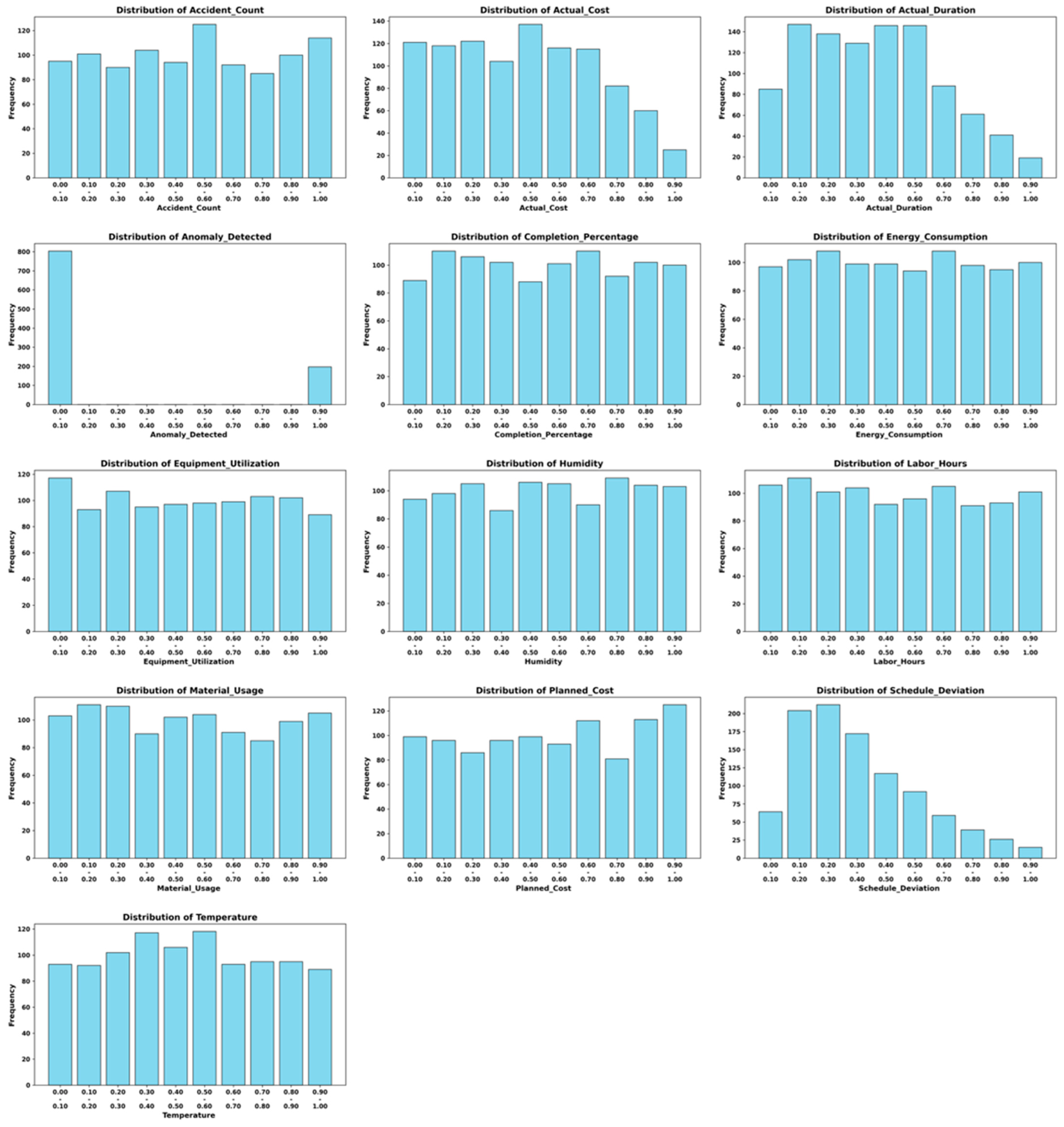
Features underwent Min-Max normalization to standardize value ranges between 0 and 1, addressing potential scale disparities among variables measured in different units. This normalization procedure ensures equal feature contribution during model training and prevents variables with larger magnitudes from dominating the learning process. This standardized data structure facilitates seamless integration with various machine learning frameworks while preserving the interpretability of individual feature contributions to model predictions. Figure 2 illustrates the distribution of numerical features after scaling.

3.5. Evaluation Metrics

To assess the performance of the predictive model, the study employed four widely adopted regression metrics: R2, RMSE, MAE, and MAPE. These metrics provide complementary insights into model accuracy, error magnitude, and interpretability. Below is a summary of the mathematical formulations and interpretations for each metric in Table 1.
Table 1 below provides the mathematical formulations for each evaluation metric used in this study, where n represents the number of observations, y i denotes the actual cost overrun values, y ˆ i represents the predicted cost overrun values, and y ¯ indicates the mean of the actual values.

4. Experimental Evaluation

To rigorously assess the efficacy of metaheuristic optimization in tuning the hyperparameters of LGBM, a systematic experimental design was employed. The objective function of each compared optimizer is defined as the mean of fivefold cross-validation performance to mitigate overfitting and ensure generalizability. Each candidate optimizer was embedded into the training process to fine-tune the LGBM parameters, producing five enhanced variants: AEFA-LGBM, CS-LGBM, DE-LGBM, POA-LGBM, and SCA-LGBM. These were compared against the baseline LGBM without optimization. Parameters of each optimizer are presented in Table 2. The baseline LGBM model was configured with a learning rate of 0.1, maximum depth of 20, and 100 estimators. For hyperparameter optimization, the search boundaries were established as follows: learning rate ranging from 0.05 to 0.5, maximum depth from 5 to 20, and number of estimators from 50 to 200. The dataset was partitioned with 70% allocated for training and 30% for testing. Due to the stochastic nature of the optimization algorithms, the entire training process was repeated across 20 independent runs, thereby capturing the variability of results and allowing for statistical characterization through the reporting of mean, standard deviation, and best-case values across multiple performance indicators. The models were evaluated on both training and testing sets using a comprehensive suite of metrics. This broad spectrum of measures ensures that the analysis goes beyond accuracy alone and includes robustness, error distribution, and interpretability of model performance.
The training outcomes in Table 3 reveal the immediate benefits of metaheuristic hyperparameter tuning, bold indicates the best value. The optimized LGBM variants consistently outperformed the baseline, demonstrating markedly improved fitting ability. While the baseline LGBM achieved an R2 of 0.9768, all optimized versions exceeded 0.994, signifying that the optimization process enabled the models to capture nearly all variance in the training data. This improvement was mirrored in the RMSE and MAE values, where metaheuristic-enhanced models reported significantly lower errors. Notably, SCA-LGBM produced the lowest average MAE (0.0068) and also recorded an impressively low RMSE (0.0110), indicating superior precision in capturing underlying patterns. A further strength of the optimized models lies in their stability. The reported standard deviations across metrics were minimal, underscoring the consistency of the metaheuristic-driven frameworks over repeated runs. In contrast, the baseline LGBM not only showed inferior averages but also exhibited greater variability, particularly in error-based metrics, suggesting its sensitivity to suboptimal parameter settings. These results underscore the value of metaheuristics in guiding the search process toward globally competitive solutions that reduce the risks of underfitting and overfitting. The true test of model performance, however, lies in the ability to generalize beyond the training data.
Table 4 presents the testing results, where again the superiority of the optimized frameworks is evident, bold indicates the best value. All metaheuristic-enhanced models achieved average R2 values around 0.978, compared to the baseline’s lower value of 0.959. This demonstrates that the optimization mechanisms not only improved the in-sample performance but also transferred predictive precision to unseen data.
The RMSE and MAE metrics further illustrate this consistency. POA-LGBM in particular stood out by achieving the lowest RMSE (0.0304) and a competitive MAE (0.0233), suggesting that its search dynamics facilitated a balanced trade-off between bias reduction and variance control. Similarly, DE-LGBM and AEFA-LGBM achieved comparably strong results, reinforcing the effectiveness of evolutionary-inspired search strategies in exploring the hyperparameter landscape. Interestingly, while the baseline LGBM exhibited a superficially favorable MAPE (20.97%) relative to the optimized models (≈30%), this outcome was coupled with MAE and high variance, which undermines its reliability. This discrepancy highlights the limitations of relying on a single percentage-based metric, as improvements in one measure may mask instability or imbalances in overall predictive behavior. The experimental findings provide robust evidence that metaheuristic optimization significantly enhances the predictive capability and robustness of LGBM. All optimized variants reduced the error metrics and achieved more stable outcomes than the baseline. The training–testing comparison also indicates that the improvements were not a result of overfitting; rather, the optimized models generalized well across independent runs and unseen data.
When comparing among the metaheuristic approaches, POA-LGBM emerged as the best performer. It demonstrated the highest average R2 in the testing phase (0.9786), the lowest RMSE, and strong stability across independent trials. This outcome can be attributed to POA’s exploration–exploitation balance, which is particularly well-suited for navigating the complex hyperparameter search space of LGBM. DE-LGBM and AEFA-LGBM followed closely, offering competitive performance with marginally higher errors. CS-LGBM and SCA-LGBM also performed significantly better than the baseline, though with slightly less consistency in certain metrics. The implications of these findings are twofold. First, they confirm that metaheuristic optimization provides a powerful mechanism to unlock the full potential of ensemble-based learners like LGBM, especially when tasked with complex prediction problems. Second, they demonstrate that the choice of optimization strategy is not inconsequential: while all metaheuristics outperformed the baseline, certain algorithms, particularly POA, achieved a superior balance of accuracy, stability, and generalization.
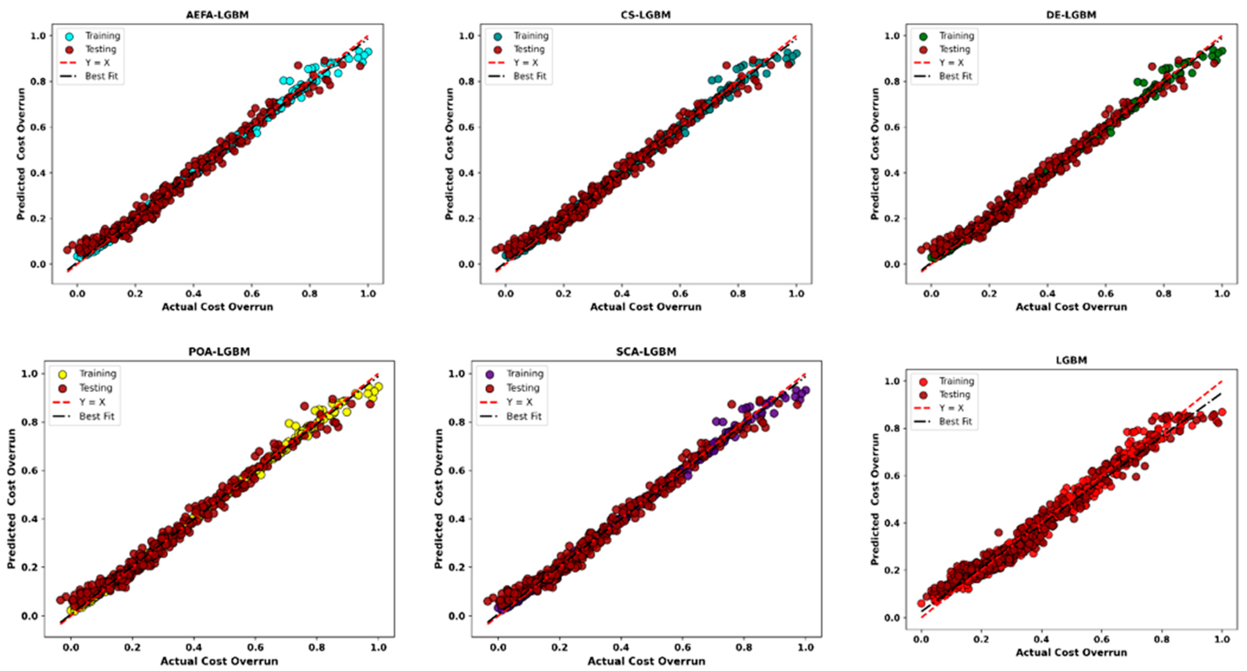
The scatter plots in Figure 3 further reinforce these conclusions by illustrating predicted versus actual cost overruns for the best-performing runs. For the optimized models, data points aligned closely with the ideal line (Y = X), and the fitted regression lines (black dashed) almost perfectly overlapped with the ideal line, indicating strong agreement between the predictions and ground truth. AEFA-LGBM, CS-LGBM, DE-LGBM, and SCA-LGBM exhibited tight clustering of training and testing points, underscoring both accuracy and consistency. AEFA-LGBM stands out by the densest clustering around the ideal line, with minimal dispersion at extreme values, reflecting its superior balance of bias and variance. As seen in Table 4, POA-LGBM exhibited more accurate prediction based on average performance, demonstrating more stable and repeatable prediction. In contrast, the baseline LGBM displayed greater scatter, with noticeable deviations particularly at higher cost overrun values. This divergence highlights the limitations of manually set hyperparameters and confirms the necessity of optimization.
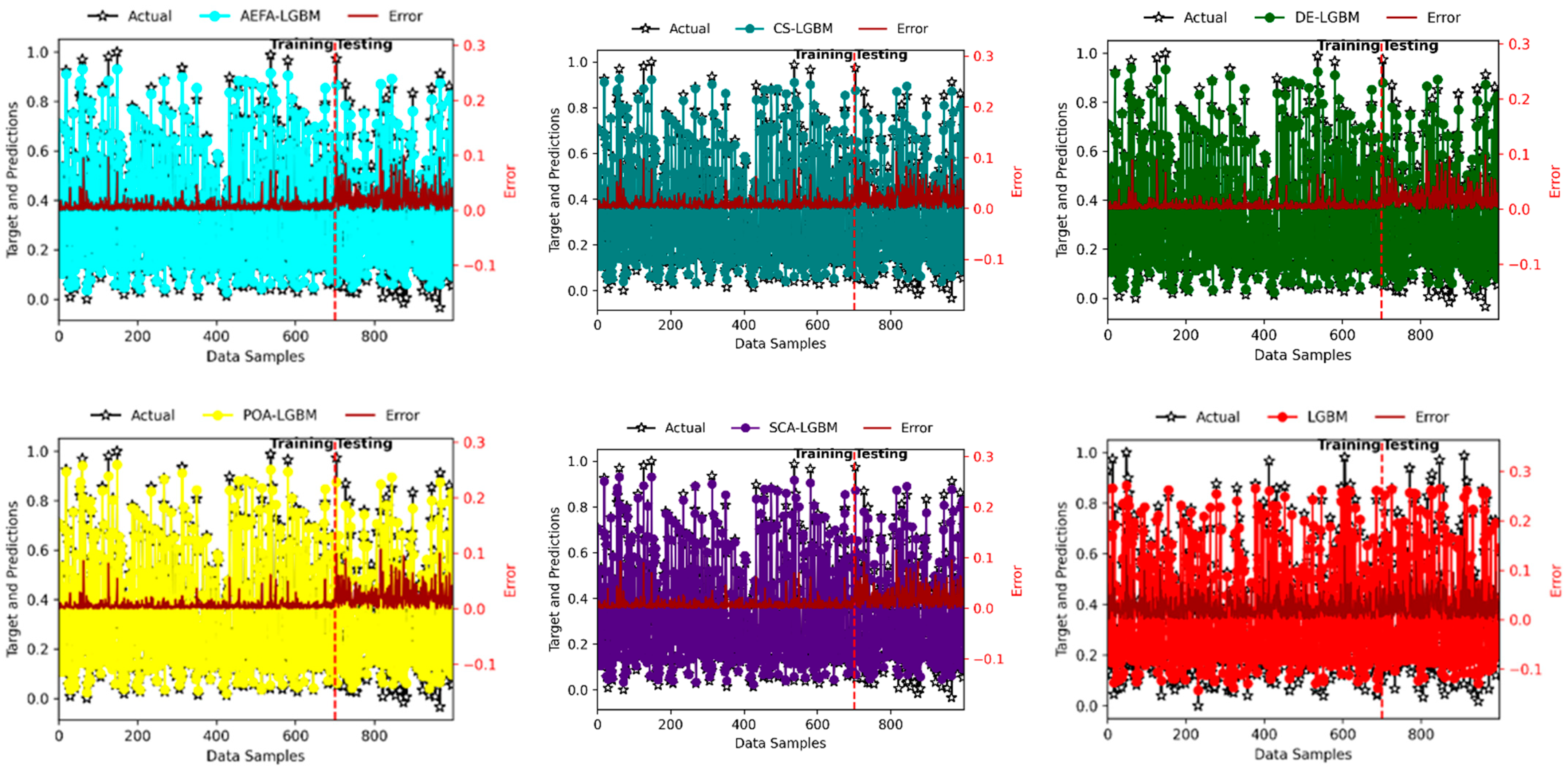
Figure 4 illustrates the prediction–target alignment alongside the absolute error distributions for the best test run of each model, with results from both the training and testing phases displayed. The plot provides a granular view of model performance, capturing how well predictions align with the actual cost overrun values and where discrepancies emerge across the sample space. Across all optimized LGBM variants, the predicted values aligned closely with the actual observations, with only minor deviations reflected in the dark-red absolute error trajectories. The error remained consistently bounded within a narrow range, confirming that metaheuristic optimization not only enhances average accuracy but also stabilizes performance across diverse samples. AEFA-LGBM and DE-LGBM, for instance, showed highly uniform error bands, with fluctuations tightly constrained around the baseline. This indicates that their optimization strategies successfully minimize outlier deviations. POA-LGBM once again demonstrated the strongest balance of accuracy and stability. The prediction curve almost perfectly overlapped the actual data across both training and testing regions, while the absolute error line remained exceptionally flat. This reinforces earlier quantitative findings (highest mean R2 and lowest RMSE during testing) and scatter plot evidence (tight clustering around the ideal prediction line). The error consistency highlights POA-LGBM’s capacity to generalize effectively while minimizing overfitting, a property particularly valuable in practical cost overrun prediction tasks where reliability is critical. In comparison, the baseline LGBM displayed substantially larger deviations. The prediction trajectory diverged more frequently from the actual data, and the absolute error line exhibited pronounced fluctuations. These inconsistencies corroborate the higher RMSE and variance reported in the numerical results, demonstrating that without optimization, LGBM is less capable of maintaining a reliable performance across varying data ranges.
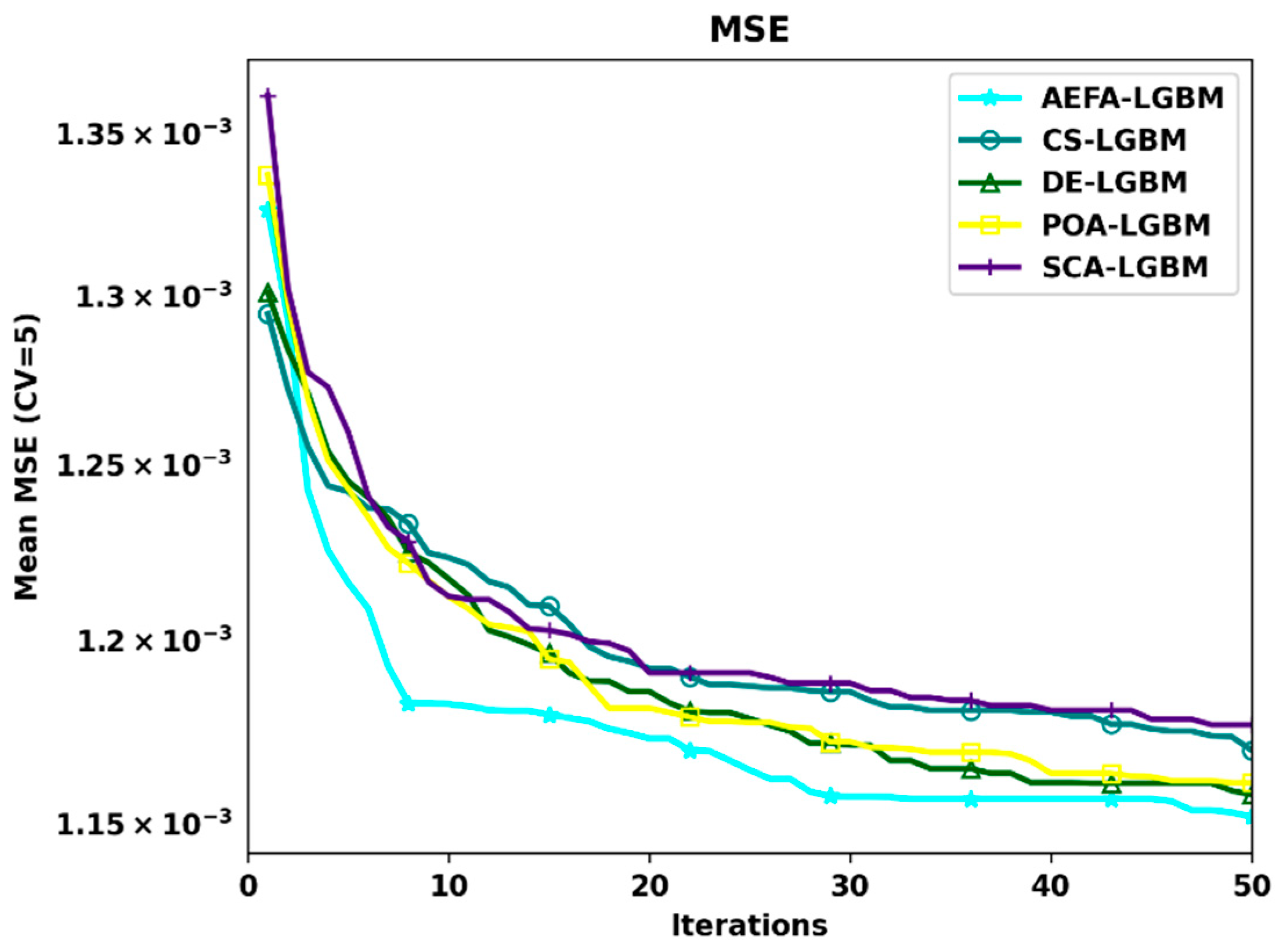
The convergence curves in Figure 5 present the trajectory of the mean cross-validation MSE across 20 independent runs for each metaheuristic-enhanced LGBM. These curves provide valuable insights into the optimization dynamics, including convergence speed, stability, and the ability to escape poor local optima. All metaheuristic variants demonstrated a rapid decline in MSE during the initial iterations, indicating effective exploration of the hyperparameter space. Within the first 30 iterations, each algorithm achieved substantial reductions in error, reflecting their capacity to quickly identify promising parameter regions. Beyond this initial phase, the trajectories flattened, suggesting a shift from exploration to exploitation as the algorithms refined their search around high-quality solutions. AEFA-LGBM exhibited the fastest convergence and ultimately achieved the lowest mean error, highlighting its strong capability for early exploitation. This explains the competitive training performance reported. POA-LGBM and DE-LGBM also converged effectively, reaching similarly low error plateaus but with a slightly slower early phase descent compared to AEFA. This more gradual convergence suggests that POA and DE balance exploration and exploitation more evenly, a property that aligns with their superior generalization performance during testing. In contrast, CS-LGBM and SCA-LGBM showed slower convergence and stabilized at marginally higher MSE values. While they outperformed the baseline LGBM by a wide margin, their optimization dynamics suggest less efficient search behavior, potentially limiting their ability to fine-tune hyperparameters to the same precision as AEFA, DE, or POA. Nonetheless, their stability across iterations indicates that once convergence is reached, the solutions remain consistent and reproducible.
The bar chart in Figure 6 illustrates the mean computational time (in seconds) over 20 independent runs for all competing optimization models. POA-LGBM exhibited the highest average runtime. The SCA-LGBM and DE-LGBM models also required relatively longer computation times due to their population-based nature. In contrast, AOA-LGBM and AEFA-LGBM demonstrated notably shorter mean runtimes, indicating faster convergence and reduced computational overhead. While the POA-LGBM incurred a marginally higher computational cost, the gain in prediction accuracy and stability justifies the trade-off, underscoring its efficiency in balancing optimization intensity and predictive robustness.
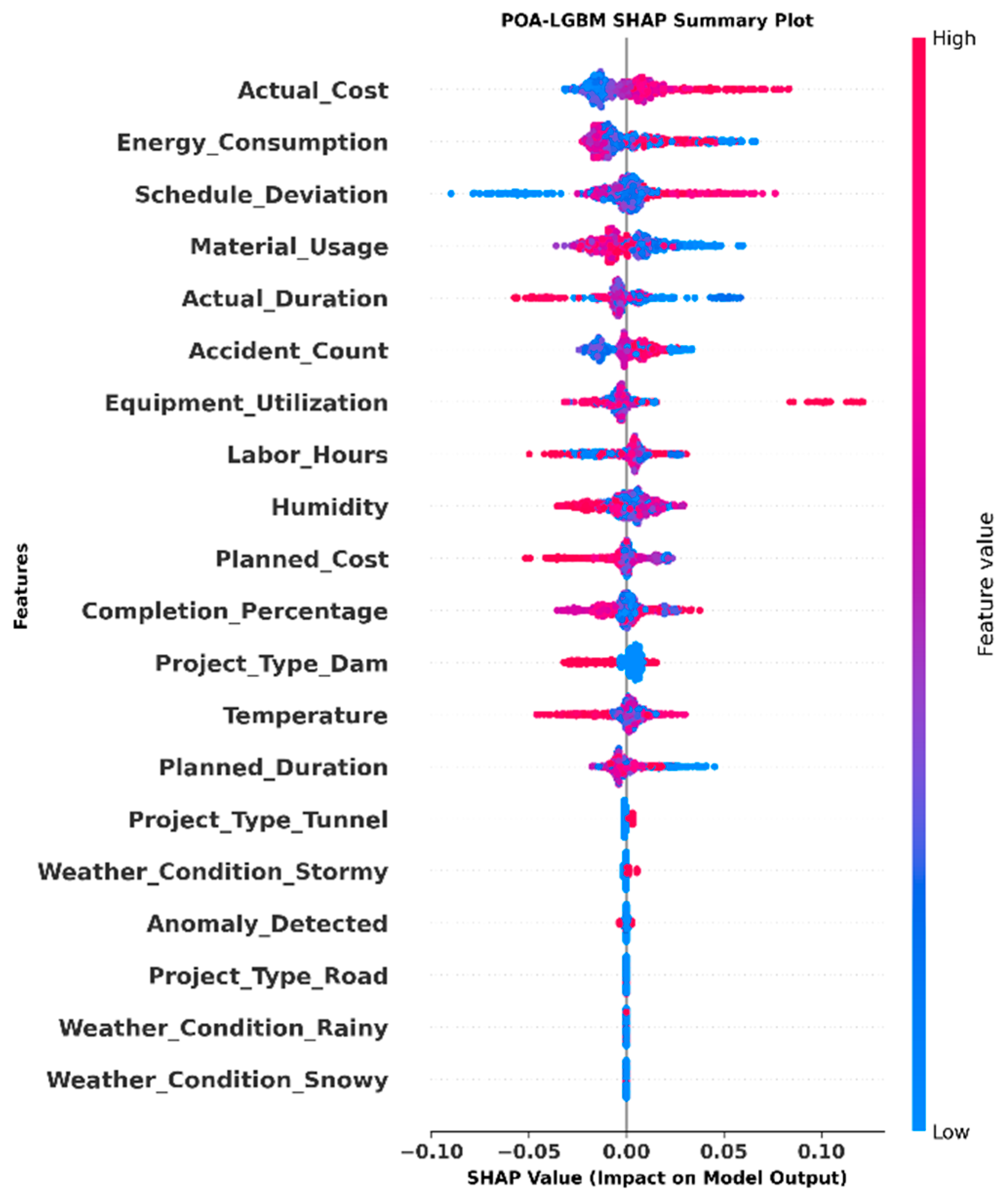
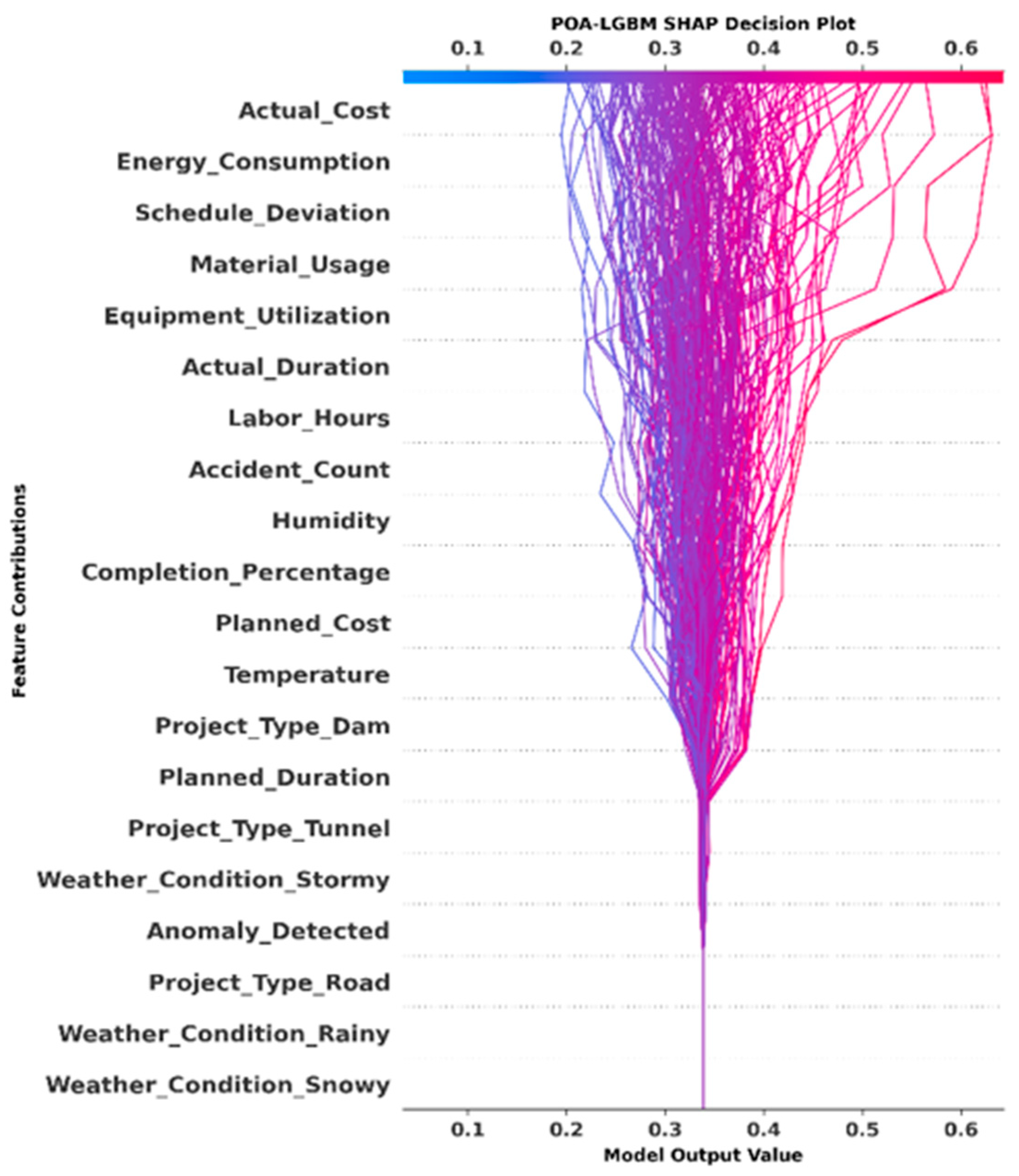
To complement the quantitative performance analysis, SHAPs were employed to interpret the decision-making process of the best-performing model, POA-LGBM. SHAPs provides a unified measure of feature contributions to the model’s predictions, allowing both global and local interpretability.
The SHAPs summary plot in Figure 7 reveals that Actual_Cost emerged as the most influential variable, exerting the highest positive and negative impact on the predicted cost overruns. This dominance aligns with domain expectations, as historical cost profiles directly inform the likelihood of future overruns. Energy_Consumption and Schedule_Deviation followed closely, highlighting the centrality of resource intensity and project scheduling in driving cost inefficiencies. The relatively wide spread of SHAPs values indicates that both high and low feature values exert strong directional influence, meaning that projects with unusual energy demand or significant schedule slippage are particularly prone to overruns.
Other variables such as Material_Usage, Actual_Duration, and Accident_Count also contributed significantly, underscoring the interplay between material allocation, timeline efficiency, and workplace safety. Notably, operational indicators like Equipment_Utilization and Labor_Hours carried moderate influence, reflecting their role as secondary determinants that amplify or mitigate cost pressures. In contrast, contextual factors such as Weather_Conditions and project-type variables displayed lower SHAPs magnitudes, suggesting that while they contribute, their effect was less consistent compared to direct cost, schedule, and resource variables.
The SHAPs decision plot in Figure 8 provides a trajectory of how features cumulatively shape predictions for individual samples. The left-to-right movement shows that predictions generally start from a baseline expectation and are progressively adjusted by key drivers. Actual_Cost and Energy_Consumption consistently shifted predictions upward, reinforcing their strong positive association with overruns. Conversely, features like Completion_Percentage and Planned_Cost often pulled predictions downward, reflecting their stabilizing effect when project progress aligns with expectations. Beyond global interpretability, the SHAPs findings offer direct managerial implications for cost control. For instance, consistently high SHAPs values associated with Actual Cost and Energy Consumption can trigger early warning thresholds within digital dashboards, prompting managers to review procurement efficiency or energy usage intensity. Similarly, a high SHAPs contribution from Schedule Deviation may signal potential downstream cost inflation, allowing for proactive schedule adjustments or contractual renegotiations before overruns materialize. In real-world deployment, these SHAP-based insights can be integrated into BIM or Digital Twin systems, enabling the real-time visualization of cost risk zones and dynamic prioritization of corrective actions. Consequently, SHAPs not only enhance interpretability, but also empower project managers to transform predictive analytics into timely, data-driven preventive strategies against escalating project costs.

5. Conclusions

This study introduced a comprehensive framework for enhancing the predictive capability of LGBM through metaheuristic-based hyperparameter optimization. Five swarm and evolutionary algorithms, namely AEFA, CS, DE, POA, and SCA, were employed to guide the optimization process, with results evaluated over 20 independent runs using a robust fivefold cross-validation as an evaluation mechanism for training. The findings demonstrated that all optimized variants outperformed the baseline LGBM, achieving higher predictive accuracy, lower error rates, and greater stability across training and testing phases. Among the tested frameworks, POA-LGBM consistently exhibited the most balanced performance in terms of accuracy, generalization, and stability, while AEFA-LGBM showed the fastest convergence.
Beyond raw performance improvements, the integration of SHAPs interpretability highlights that the optimized models are not black boxes. Instead, they identify intuitive and domain-relevant drivers of cost overruns, such as actual cost, energy consumption, and schedule deviation, thereby offering actionable insights for project managers. This dual emphasis on predictive strength and interpretability strengthens the case for metaheuristic-enhanced LGBM as a practical decision-support tool in managing complex project environments. Importantly, our prediction model, as shown in Figure 1, demonstrates that metaheuristic-enhanced LGBM can provide a structured approach to balance exploration and exploitation in analytical decisions through data-driven interpretability.
Despite its contributions, the study is not without limitations. First, the analysis was conducted on a single dataset, which, while rich and representative, may limit the generalizability of results across different industries or project types. Although the current dataset encompassed multiple construction categories including residential, commercial, and infrastructure projects, future work will involve testing the POA-LGBM framework on regional and sectoral datasets to evaluate its transferability across diverse contexts. Such cross-domain validation will help quantify robustness to geographic, climatic, and regulatory variability. In practical terms, real-world deployment may face challenges such as limited data availability, model scalability, and stakeholder acceptance. To address these, the framework can be expanded through federated learning architectures that preserve data privacy across firms and incremental retraining pipelines to adapt to evolving project data.
Second, although multiple metaheuristic algorithms were compared, the study did not explore hybrid or adaptive mechanisms that dynamically balance exploration and exploitation, which may yield further improvements. Finally, computational cost remains a consideration, as multiple independent runs of metaheuristic optimization are resource-intensive, potentially constraining scalability in real-world, large-scale deployments. We note that the present study provides a rigorous comparison among metaheuristic-optimized ensemble models. In future research, we plan to extend our benchmarking to include deep-learning and RL models trained under comparable conditions, thereby more fully situating the POA-LGBM framework within the broader advanced AI landscape of cost-overrun prediction and digital project management analytics.
Future research should address these limitations along several directions. Extending the evaluation to multi-domain datasets including infrastructure, manufacturing, and energy systems would validate the robustness and adaptability of the proposed framework. Additionally, integrating hybrid or multi-objective metaheuristics could further enhance optimization efficiency by jointly considering the accuracy, computation time, and interpretability. From a practical standpoint, embedding the proposed models into real-time monitoring and decision-support systems could transform predictive modeling into proactive cost overrun management. Finally, expanding the research to ensemble approaches that combine multiple optimized learners could yield even greater robustness and accuracy in highly uncertain environments.

Author Contributions

J.M.M.L.: Conceptualization, Methodology, Formal Analysis, Original Draft, O.S.O.: Supervision, Resources, Editing. All authors have read and agreed to the published version of the manuscript.

Funding

The authors declare that no funding was received.

Data Availability Statement

The data obtained through the experiments are available upon request from the corresponding author.

Conflicts of Interest

The authors declare no conflict of interest.

References

  1. Atkinson, R. Project management: Cost, time and quality, two best guesses and a phenomenon, its time to accept other success criteria. Int. J. Proj. Manag. 1999, 17, 337–342. [Google Scholar] [CrossRef]
  2. Bryde, D.J.; Brown, D. The Influence of a Project Performance Measurement System on the Success of a Contract for Maintaining Motorways and Trunk Roads. Proj. Manag. J. 2004, 35, 57–65. [Google Scholar] [CrossRef]
  3. Ahiaga-Dagbui, D.D.; Smith, S.D. Dealing with construction cost overruns using data mining. Constr. Manag. Econ. 2014, 32, 682–694. [Google Scholar] [CrossRef]
  4. Osei-Asibey, D.; Ayarkwa, J.; Baah, B.; Afful, A.E.; Anokye, G.; Nkrumah, P.A. Impact of time-based delay on public-private partnership (PPP) construction project delivery: Construction stakeholders’ perspective. J. Financ. Manag. Prop. Constr. 2024, 30, 88–110. [Google Scholar] [CrossRef]
  5. Wang, Y.; Chen, J.; Liu, J.; Zhou, C. Investors’ exit timing of PPP projects based on escalation of commitment. PLoS ONE 2021, 16, e0253394. [Google Scholar] [CrossRef]
  6. Love, P.E.D.; Sing, M.C.P.; Ika, L.A.; Newton, S. The cost performance of transportation projects: The fallacy of the Planning Fallacy account. Transp. Res. Part. A Policy Pract. 2019, 122, 1–20. [Google Scholar] [CrossRef]
  7. Melaku Belay, S.; Tilahun, S.; Yehualaw, M.; Matos, J.; Sousa, H.; Workneh, E.T. Analysis of Cost Overrun and Schedule Delays of Infrastructure Projects in Low Income Economies: Case Studies in Ethiopia. Adv. Civ. Eng. 2021, 2021, 4991204. [Google Scholar] [CrossRef]
  8. Terrill, M.; Emslie, O.; Moran, G. The Rise of Mega-Projects: Counting the Costs. 2020. Available online: https://trid.trb.org/View/1756433 (accessed on 16 September 2025).
  9. Kadiri, D.S.; Onabanjo, B.O. Cost and Time Overruns in Building Projects Procured Using Traditional Contracts in Nigeria. J. Sustain. Dev. 2017, 10, p234. [Google Scholar] [CrossRef]
  10. Andrić, J.M.; Lin, S.; Cheng, Y.; Sun, B. Determining Cost and Causes of Overruns in Infrastructure Projects in South Asia. Sustainability 2024, 16, 11159. [Google Scholar] [CrossRef]
  11. Flyvbjerg, B.; Holm, M.S.; Buhl, S. Underestimating Costs in Public Works Projects: Error or Lie? J. Am. Plan. Assoc. 2002, 68, 279–295. [Google Scholar] [CrossRef]
  12. Bhattacharyya, A.; Yoon, S.; Weidner, T.J.; Hastak, M. Purdue Index for Construction Analytics: Prediction and Forecasting Model Development. J. Manag. Eng. 2021, 37, 04021052. [Google Scholar] [CrossRef]
  13. Coffie, G.H.; Cudjoe, S.K.F. Toward predictive modelling of construction cost overruns using support vector machine techniques. Cogent Eng. 2023, 10, 2269656. [Google Scholar] [CrossRef]
  14. Plebankiewicz, E. Model of Predicting Cost Overrun in Construction Projects. Sustainability 2018, 10, 4387. [Google Scholar] [CrossRef]
  15. ForouzeshNejad, A.A.; Arabikhan, F.; Aheleroff, S. Optimizing Project Time and Cost Prediction Using a Hybrid XGBoost and Simulated Annealing Algorithm. Machines 2024, 12, 867. [Google Scholar] [CrossRef]
  16. Shreena Global Construction Futures. Oxford Economics 2023. Available online: https://www.oxfordeconomics.com/resource/global-construction-futures/ (accessed on 16 September 2025).
  17. Shamim, M.M.I.; Hamid, A.B.B.A.; Nyamasvisva, T.E.; Rafi, N.S.B. Advancement of Artificial Intelligence in Cost Estimation for Project Management Success: A Systematic Review of Machine Learning, Deep Learning, Regression, and Hybrid Models. Modelling 2025, 6, 35. [Google Scholar] [CrossRef]
  18. Ke, G.; Meng, Q.; Finley, T.; Wang, T.; Chen, W.; Ma, W.; Ye, Q.; Liu, T.-Y. LightGBM: A Highly Efficient Gradient Boosting Decision Tree. In Proceedings of the Advances in Neural Information Processing Systems, Long Beach, CA, USA, 4–9 December 2017; Guyon, I., Luxburg, U.V., Bengio, S., Wallach, H., Fergus, R., Vishwanathan, S., Garnett, R., Eds.; Curran Associates, Inc.: Red Hook, NY, USA, 2017; Volume 30. Available online: https://proceedings.neurips.cc/paper_files/paper/2017/file/6449f44a102fde848669bdd9eb6b76fa-Paper.pdf (accessed on 5 September 2025).
  19. Anonto, H.Z.; Hossain, M.I.; Momo, M.; Shufian, A.; Kumar Roy, A.; Ashraf, M.S.; Islam, R. Optimizing Energy Consumption Prediction Using Hybrid LightGBM and XGBoost: Integrating Heterogeneous Data for Smart Grid Management. In Proceedings of the 2025 IEEE Region 10 Symposium (TENSYMP), Christchurch, New Zealand, 10 July 2025; pp. 1–8. [Google Scholar] [CrossRef]
  20. Zhang, J.; Mucs, D.; Norinder, U.; Svensson, F. LightGBM: An Effective and Scalable Algorithm for Prediction of Chemical Toxicity-Application to the Tox21 and Mutagenicity Data Sets. J. Chem. Inf. Model. 2019, 59, 4150–4158. [Google Scholar] [CrossRef] [PubMed]
  21. Gan, M.; Pan, S.; Chen, Y.; Cheng, C.; Pan, H.; Zhu, X. Application of the Machine Learning LightGBM Model to the Prediction of the Water Levels of the Lower Columbia River. J. Mar. Sci. Eng. 2021, 9, 496. [Google Scholar] [CrossRef]
  22. Duan, S.; Huang, S.; Bu, W.; Ge, X.; Chen, H.; Liu, J.; Luo, J. LightGBM Low-Temperature Prediction Model Based on LassoCV Feature Selection. Math. Probl. Eng. 2021, 2021, 1776805. [Google Scholar] [CrossRef]
  23. Zhou, F.; Hu, S.; Du, X.; Wan, X.; Lu, Z.; Wu, J. Lidom: A Disease Risk Prediction Model Based on LightGBM Applied to Nursing Homes. Electronics 2023, 12, 1009. [Google Scholar] [CrossRef]
  24. Zhou, Y.; Wang, W.; Wang, K.; Song, J. Application of LightGBM Algorithm in the Initial Design of a Library in the Cold Area of China Based on Comprehensive Performance. Buildings 2022, 12, 1309. [Google Scholar] [CrossRef]
  25. Budak, İ. Prediction of Water Quality’s pH value using Random Forest and LightGBM Algorithms. MEMBA Su Bilim. Derg. 2025, 11, 42–49. [Google Scholar] [CrossRef]
  26. Xi, X. The role of LightGBM model in management efficiency enhancement of listed agricultural companies. Appl. Math. Nonlinear Sci. 2023, 9, 1–14. [Google Scholar] [CrossRef]
  27. Wang, D.; Zhang, Y.; Zhao, Y. LightGBM: An Effective miRNA Classification Method in Breast Cancer Patients. In Proceedings of the 2017 International Conference on Computational Biology and Bioinformatics, in ICCBB ’17, Newark, NJ, USA, 18–20 October 2017; Association for Computing Machinery: New York, NY, USA, 2017; pp. 7–11. [Google Scholar] [CrossRef]
  28. Li, S.; Jin, N.; Dogani, A.; Yang, Y.; Zhang, M.; Gu, X. Enhancing LightGBM for Industrial Fault Warning: An Innovative Hybrid Algorithm. Processes 2024, 12, 221. [Google Scholar] [CrossRef]
  29. Shirali, M.; Hatamiafkoueieh, J.; Razoumny, Y.; Olegovich, D.D. Accuracy enhancement in land subsidence prediction using lightgbm and metaheuristic optimization. Earth Sci. Inf. 2025, 18, 435. [Google Scholar] [CrossRef]
  30. Lundberg, S.M.; Lee, S.-I. A Unified Approach to Interpreting Model Predictions. In Proceedings of the Advances in Neural Information Processing Systems, Long Beach, CA, USA, 4–9 December 2017; Guyon, I., Luxburg, U.V., Bengio, S., Wallach, H., Fergus, R., Vishwanathan, S., Garnett, R., Eds.; Curran Associates, Inc.: Red Hook, NY, USA, 2017; Volume 30. Available online: https://proceedings.neurips.cc/paper_files/paper/2017/file/8a20a8621978632d76c43dfd28b67767-Paper.pdf (accessed on 5 September 2025).
  31. Janizadeh, S.; Thi Kieu Tran, T.; Bateni, S.M.; Jun, C.; Kim, D.; Trauernicht, C.; Heggy, E. Advancing the LightGBM approach with three novel nature-inspired optimizers for predicting wildfire susceptibility in Kauaʻi and Molokaʻi Islands, Hawaii. Expert. Syst. Appl. 2024, 258, 124963. [Google Scholar] [CrossRef]
  32. Nazier, M.M.; Gomaa, M.M.; Abdallah, M.M.; Sayed, A. Arabic Sentiment Analysis Using Optuna Hyperparameter Optimization and Metaheuristics Feature Selection to Improve Performance of LightGBM. Int. J. Adv. Comput. Sci. Appl. 2025, 16, 553. [Google Scholar] [CrossRef]
  33. Akinola, I.T.; Sun, Y.; Adebayo, I.G.; Wang, Z. Daily peak demand forecasting using Pelican Algorithm optimised Support Vector Machine (POA-SVM). Energy Rep. 2024, 12, 4438–4448. [Google Scholar] [CrossRef]
  34. Al mnaseer, R.; Al-Smadi, S.; Al-Bdour, H. Machine learning-aided time and cost overrun prediction in construction projects: Application of artificial neural network. Asian J. Civ. Eng. 2023, 24, 2583–2593. [Google Scholar] [CrossRef]
  35. Cheng, M.-Y.; Vu, Q.-T.; Gosal, F.E. Hybrid deep learning model for accurate cost and schedule estimation in construction projects using sequential and non-sequential data. Autom. Constr. 2025, 170, 105904. [Google Scholar] [CrossRef]
  36. Elmasry, N.H.; Elshaarawy, M.K. Hybrid metaheuristic optimized Catboost models for construction cost estimation of concrete solid slabs. Sci. Rep. 2025, 15, 21612. [Google Scholar] [CrossRef] [PubMed]
  37. Coffie, G.H.; Cudjoe, S.K.F. Using extreme gradient boosting (XGBoost) machine learning to predict construction cost overruns. Int. J. Constr. Manag. 2024, 24, 1742–1750. [Google Scholar] [CrossRef]
  38. Mahmoodzadeh, A.; Nejati, H.R.; Mohammadi, M. Optimized machine learning modelling for predicting the construction cost and duration of tunnelling projects. Autom. Constr. 2022, 139, 104305. [Google Scholar] [CrossRef]
  39. Doulabi, R.Z. A Hybrid Machine Learning and Metaheuristic Framework for Optimizing Time and Cost in Hospital Construction Projects. Int. J. Intell. Syst. Appl. Eng. 2025, 13, 385–394. [Google Scholar]
  40. Han, K.; Wang, T.; Liu, W.; Li, C.; Xian, X.; Yang, Y. Construction cost prediction model for agricultural water conservancy engineering based on BIM and neural network. Sci. Rep. 2025, 15, 24271. [Google Scholar] [CrossRef]
  41. Almahameed, B.A.; Bisharah, M. Applying Machine Learning and Particle Swarm Optimization for predictive modeling and cost optimization in construction project management. Asian J. Civ. Eng. 2024, 25, 1281–1294. [Google Scholar] [CrossRef]
  42. Trojovský, P.; Dehghani, M. Pelican Optimization Algorithm: A Novel Nature-Inspired Algorithm for Engineering Applications. Sensors 2022, 22, 855. [Google Scholar] [CrossRef]
  43. Mahmoudzadeh, A.; Amiri-Ramsheh, B.; Atashrouz, S.; Abedi, A.; Abuswer, M.A.; Ostadhassan, M.; Mohaddespour, A.; Hemmati-Sarapardeh, A. Modeling CO2 solubility in water using gradient boosting and light gradient boosting machine. Sci. Rep. 2024, 14, 13511. [Google Scholar] [CrossRef]
  44. Sun, X. Application of an improved LightGBM hybrid integration model combining gradient harmonization and Jacobian regularization for breast cancer diagnosis. Sci. Rep. 2025, 15, 2569. [Google Scholar] [CrossRef] [PubMed]
  45. BIM-AI Integrated Dataset. Available online: https://www.kaggle.com/datasets/ziya07/bim-ai-integrated-dataset (accessed on 4 September 2025).
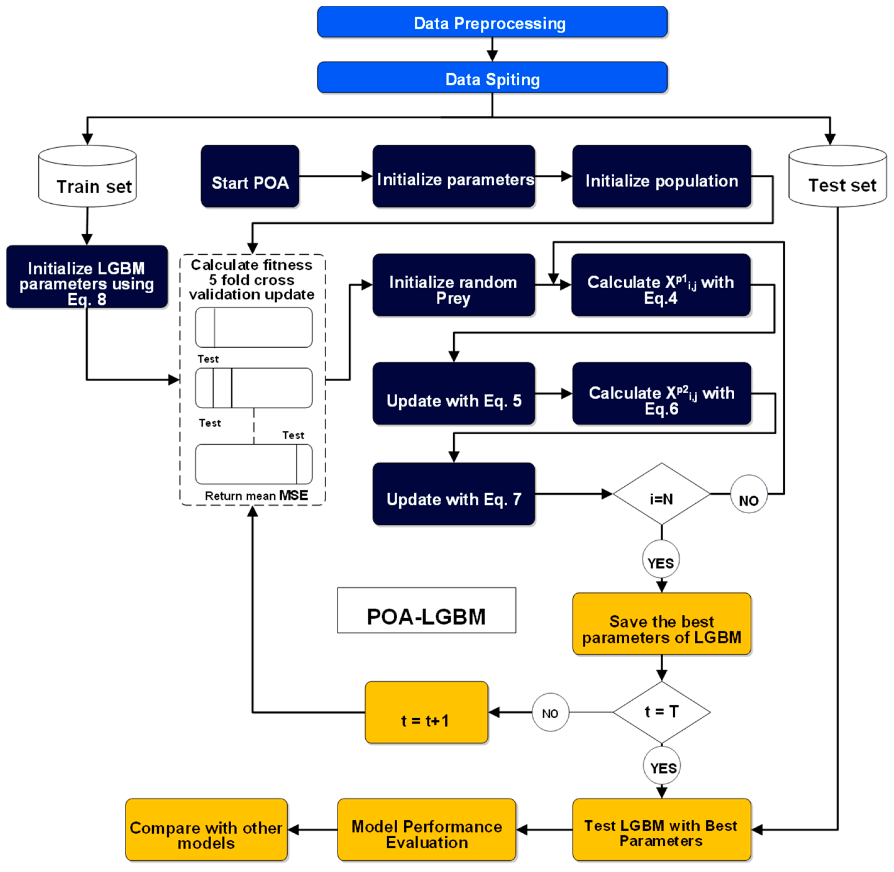
Figure 1. POA-LGBM prediction model.
Systems 13 01047 g001
Figure 2. Distribution of numerical features.
Systems 13 01047 g002
Figure 3. Predicted vs. actual of models.
Systems 13 01047 g003
Figure 4. Error plots of the prediction model.
Systems 13 01047 g004
Figure 5. Convergence plot.
Systems 13 01047 g005
Figure 6. Runtime of compared model.
Systems 13 01047 g006
Figure 7. SHAPs analysis of impact of features.
Systems 13 01047 g007
Figure 8. SHAPs analysis of POA-LGBM decision during prediction.
Systems 13 01047 g008
Table 1. Evaluation metrics.
MetricMathematical FormulationTypical Range & Note
R 2 R 2 = 1 i = 1 n     y i y ˆ i 2 i = 1 n     y i y 2 < R 2 1 (values < 0 occur when the model underperforms the mean predictor)
RMSE (Root-Mean-Squared Error) R M S E = 1 n i = 1 n     y i y ˆ i 2 [ 0 , ) ; lower is better
MAE (Mean Absolute Error) MAE = 1 n i = 1 n   y i y ˆ i [ 0 , ) ; lower is better
MAPE (Mean Absolute Percentage Error) M A P E = 100 n i = 1 n     y i y ˆ i y i [ 0 , ) % ; lower is better
Table 2. Optimization algorithms parameters.
AlgorithmsParameter Setting
AEFA k 0 = 500 , γ = 30
CS P a = 0.25 , r = 0.05
DE F = 0.5 ,   C R = 0.7
POAR = 0.2
SCA a = 2
Table 3. Training results of 20 independent runs.
AEFA-LGBMCS-LGBMDE-LGBMPOA-LGBMSCA-LGBMLGBM
R2AVG0.995600.997140.997220.997110.997170.97683
STD9.6721 × 10−41.2766 × 10−38.1976 × 10−49.7025 × 10−41.6715 × 10−31.6387 × 10⁻³
Best0.997510.999180.998540.998520.999420.97984
RMSEAVG1.4254 × 10−21.1258 × 10−21.1265 × 10−21.1472 × 10−21.1014 × 10−23.1964 × 10⁻²
STD1.5742 × 10−32.5896 × 10−31.6884 × 10−31.8294 × 10−33.2976 × 10−39.4009 × 10⁻⁴
Best1.0778 × 10−26.1850 × 10−38.2730 × 10−38.3130 × 10−35.2050 × 10−33.0067 × 10⁻²
MAEAVG9.2692 × 10−37.0936 × 10−37.0767 × 10−37.1763 × 10−36.8588 × 10−32.4781 × 10⁻²
STD1.1983 × 10−31.9636 × 10−31.3036 × 10−31.4814 × 10−32.6748 × 10−36.6421 × 10⁻⁴
Best6.5610 × 10−33.2520 × 10−34.6230 × 10−34.6130 × 10−32.3110 × 10−32.3480 × 10⁻²
MAPEAVG6.43224.68094.60344.70924.48521.3997 × 101
STD9.4115 × 10−11.50751.03211.12192.02362.8684
Best4.29451.81432.77542.74951.12171.1578 × 101
Table 4. Testing results of 20 independent runs.
AEFA-LGBMCS-LGBMDE-LGBMPOA-LGBMSCA-LGBMLGBM
R2AVG0.978480.978370.978450.978560.978220.95919
STD7.7721 × 10−57.0533 × 10−46.3666 × 10−43.8363 × 10−47.1151 × 10−44.6021 × 10⁻³
Best0.978270.976690.976830.977940.976370.95019
RMSEAVG3.0493 × 10−23.0566 × 10−23.0513 × 10−23.0432 × 10−23.0671 × 10−24.2477 × 10⁻²
STD5.4949 × 10−54.9664 × 10−44.4780 × 10−42.7326 × 10−44.9791 × 10−42.9544 × 10⁻³
Best3.0415 × 10−22.9673 × 10−22.9956 × 10−22.9762 × 10−22.9799 × 10−23.7379 × 10⁻²
MAEAVG2.3193 × 10−22.3427 × 10−22.3414 × 10−22.3267 × 10−22.3482 × 10−23.3356 × 10⁻²
STD5.6641 × 10−54.6134 × 10−44.5545 × 10−42.3405 × 10−44.5953 × 10−42.4926 × 10⁻³
Best2.3104 × 10−22.2732 × 10−22.2902 × 10−22.2804 × 10−22.2655 × 10−22.8801 × 10⁻²
MAPEAVG3.0828 × 1013.0661 × 1013.0439 × 1013.0567 × 1013.0702 × 1012.0975 × 101
STD1.3558 × 10−16.4876 × 10−14.4589 × 10−15.2025 × 10−17.9319 × 10−17.9711
Best3.0639 × 1012.9467 × 1012.9813 × 1012.9165 × 1012.9413 × 1011.2617 × 101
Disclaimer/Publisher’s Note: The statements, opinions and data contained in all publications are solely those of the individual author(s) and contributor(s) and not of MDPI and/or the editor(s). MDPI and/or the editor(s) disclaim responsibility for any injury to people or property resulting from any ideas, methods, instructions or products referred to in the content.