Article

Trajectory Prediction for Powered Two-Wheelers in Mixed Traffic Scenes: An Enhanced Social-GAT Approach

1
School of Architecture and Transportation Engineering, Guilin University of Electronic Technology, Guilin 541000, China
2
School of Artificial Intelligence, Guilin University of Electronic Technology, Guilin 541000, China
3
School of Computer Science and Information Security, Guilin University of Electronic Technology, Guilin 541000, China
*
Author to whom correspondence should be addressed.
Systems 2025, 13(11), 1036; https://doi.org/10.3390/systems13111036
Submission received: 2 October 2025 / Revised: 6 November 2025 / Accepted: 17 November 2025 / Published: 19 November 2025
(This article belongs to the Section Artificial Intelligence and Digital Systems Engineering)

Abstract

In mixed traffic scenarios involving both motorized and non-motorized participants, accurately predicting future trajectories of surrounding vehicles remains a major challenge for autonomous driving. Predicting the motion of powered two-wheelers (PTWs) is particularly difficult due to their abrupt behavioral changes and stochastic interaction patterns. To address this issue, this paper proposes an enhanced Social-GAT model with a multi-module architecture for PTW trajectory prediction. The model consists of a dual-channel LSTM encoder that separately processes position and motion features; a temporal attention mechanism to weight key historical states; and a residual-connected two-layer GAT structure to model social relationships within the interaction range, capturing interactive features between PTWs and surrounding vehicles through dynamic adjacency matrices. Finally, an LSTM decoder integrates spatiotemporal features and outputs the predicted trajectory. Experimental results on the rounD dataset demonstrate that our model achieves an outstanding ADE of 0.28, surpassing Trajectron++ by 9.68% and Social-GAN by 69.2%. It also attains the lowest RMSE values across 0.4–2.0s prediction horizons, confirming its superior accuracy and stability for PTW trajectory prediction in mixed traffic environments.

1. Introduction

With the advancement of autonomous driving technology, urban transportation will undergo a prolonged transition period characterized by mixed traffic scenarios involving both autonomous and human-driven vehicles. Accurately predicting the trajectories of surrounding vehicles has become one of the critical factors in ensuring the operational safety of autonomous cars and reducing collision risks [1]. Compared to motor vehicles, non-motorized vehicles exhibit more flexible maneuvering and weaker behavioral regularity, which poses significant challenges for autonomous driving systems in predicting their trajectories. Among these, predicting the trajectories of powered two-wheelers (PTWs) is particularly critical and challenging. This is not only because, compared to traditional bicycles, PTWs have greater mass and higher travel speeds [2], but more importantly, due to their unique dynamic characteristics: (1) high maneuverability and instability: PTWs possess a high power-to-weight ratio, leading to rapid and abrupt changes in acceleration and deceleration (high jerk), which results in highly non-linear motion patterns. (2) Narrow physical profile and lane-independence: their small size allows them to occupy any position within a lane and even travel alongside cars, making their behavior less constrained by lane markings and more unpredictable. (3) Leaning-in-curve dynamics: the unique physics of balancing and leaning during turns cause their trajectory curvature to change differently from four-wheeled vehicles.
However, most existing trajectory prediction studies treat non-motorized vehicles as a homogeneous group and rely on deep learning models to learn their “average characteristics.” This approach is inadequate, as it tends to overlook the distinct motion patterns of PTWs, leading to inaccurate prediction results [3]. Laurin et al. [4] categorized non-motorized two-wheelers into three types based on their dynamic speed profiles: conventional bicycles, electric bicycles, and speed electric bicycles. This finding underscores that treating non-motorized vehicles as a unified category may fail to capture the more dynamic motion characteristics of PTWs, which poses a significant risk to urban traffic safety. Therefore, it is necessary to study powered two-wheelers as a separate entity and, crucially, to design targeted model architectures capable of explicitly capturing these unique features.
With the advancement of artificial intelligence technologies, deep learning methods have become the mainstream approach in the field of trajectory prediction due to their exceptional capability in capturing behavioral patterns and modeling complex interactions. Among these, LSTM [5], with its carefully designed gating mechanism, effectively addresses the vanishing and exploding gradient problems that traditional RNNs encounter when processing long sequences, giving it a distinct advantage in trajectory prediction tasks. However, numerous experiments have revealed that LSTM and its variants exhibit significant limitations in interaction modeling, making it difficult to effectively capture complex interactions among multiple agents. In trajectory prediction tasks within complex traffic scenarios, these methods often struggle to achieve high efficiency and accuracy. In recent years, with the development of attention mechanisms, the LSTM-Attention architecture has emerged as one of the effective solutions for trajectory prediction. This approach can, to some extent, mitigate the shortcomings of LSTM in interaction modeling.
Graph Neural Networks (GNNs) have gained increasing attention in the field of trajectory prediction in recent years, primarily due to their strength in modeling complex interactions [6,7]. Unlike LSTM, which focuses mainly on temporal features, GNNs specialize in capturing spatial and semantic relationships among entities in traffic scenes. Although GNNs excel at interaction modeling, they suffer from drawbacks such as high computational complexity and limited adaptability to dynamic scenarios when applied to trajectory prediction. In response, Graph Attention Networks (GAT) have been proposed. As a mechanism that can be integrated into GNN architectures, GAT employs attention to focus on the most relevant features in the graph [8], thereby enabling more accurate trajectory prediction. Moreover, GAT allows each node to have distinct weights for different neighbors, effectively capturing node-level variations.
Based on the above analysis, this paper proposes an encoder–decoder trajectory prediction framework integrating LSTM, temporal attention, and GAT, specifically designed to capture the motion characteristics of PTWs. The framework combines LSTM’s ability to encode long sequences with GAT’s strength in modeling complex dynamic interactions. Meanwhile, the incorporation of temporal attention further enables the model to capture motion features at critical time steps, thereby improving its adaptability to the trajectory patterns of PTWs. The main contributions of this study are as follows:
  • This study specifically focuses on PTWs, capturing their unique motion patterns in mixed traffic scenarios. This fine-grained analysis enhances behavioral prediction accuracy, contributing to improved safety for autonomous vehicles.
  • A reinforced LSTM encoder–decoder framework integrated with graph attention is proposed. It effectively captures long-term temporal dependencies and complex interactions, achieving high-precision trajectory prediction in intricate traffic scenarios.
  • An absolute coordinate correction module is introduced to mitigate the starting point drift caused by relative coordinate output. This method significantly improves prediction accuracy on the rounD dataset.

2. Related Works

2.1. Current Research Status in Trajectory Prediction

The development of trajectory prediction research can be divided into three main stages: methods based on physical dynamics, those based on traditional machine learning, and the current mainstream deep learning approaches. These three stages exhibit clear progressive improvements in terms of prediction accuracy, computational efficiency, and scenario adaptability.
During the physics-based modeling phase, researchers proposed numerous motion models based on simplified dynamic assumptions to address the behavior prediction of road participants. Leigh et al. [9] evaluated the performance of the constant velocity model in pedestrian trajectory prediction, while Schöller et al. [10] demonstrated through experiments in linear-path scenarios that the constant velocity model outperformed neural network-based approaches. Liu et al. [11] developed a dynamics model for intelligent vehicles operating on off-road terrain, incorporating road inclination angles, and conducted trajectory tracking studies under simulated slope conditions. Although such methods are computationally efficient, they rely solely on kinematic parameters to describe vehicle motion [12], making them unsuitable for predicting highly uncertain vehicle behaviors in complex road environments. Consequently, methods such as the Kalman filter [13], Markov models [14], probabilistic models [15], and social force models [16,17] were successively introduced to better handle trajectory prediction in complex scenarios. However, these approaches require manual design, and their performance heavily depends on the researchers’ understanding and assumptions regarding dynamics and interactions [18]. As a result, while they exhibit certain advantages in short-term prediction, they struggle to cope with intricate and dynamic vehicle interactions, leading to limited prediction accuracy.
With the improvement in computational power and the increase in data availability, researchers began to explore the application of machine learning methods in the field of trajectory prediction. Classical approaches primarily include Gaussian processes, support vector machines (SVM), hidden Markov models (HMM), and dynamic Bayesian networks (DBN), among others. Rong et al. [19] proposed a data-driven, non-parametric Bayesian model based on Gaussian processes to describe the uncertainty in lateral motion, enabling real-time and high-precision prediction of ship trajectories. While SVM is effective for classification tasks, Mandalia et al. [20] were among the first to apply it to recognize lane-changing maneuvers using features such as steering wheel angle, position, and acceleration. However, the utility of this method remains limited in trajectory prediction. In contrast, hidden Markov models have demonstrated stronger performance in this domain. Zhang et al. [15] introduced a game theory-based GMM-HMM maneuver prediction model that incorporates interaction-aware factors. To further account for interactions between vehicles, dynamic Bayesian networks were developed to effectively address this need. He et al. [21] proposed a practical and efficient intention prediction method based on DBN, achieving effective recognition of lane-keeping and lane-changing intentions. Although these methods perform well in specific scenarios, they require predefined behavior categories and exhibit limited generalization capability, which laid the groundwork for the emergence of deep learning approaches.
Compared to the two aforementioned categories of methods, deep learning approaches leverage the power of artificial neural networks to learn complex patterns and relationships from large volumes of data, enabling trajectory prediction in complex scenarios while maintaining relatively low model complexity and computational cost. These methods primarily include recurrent neural networks (RNN), convolutional neural networks (CNN), attention mechanisms (AM), graph neural networks (GNN), and generative models, among others [22]. In recent years, RNN and its variants, such as LSTM [5] and GRU [23], have been widely adopted in trajectory prediction due to their ability to effectively capture temporal dependencies in sequential data, making them suitable for long-term forecasting [24]. Pool et al. [25] proposed an RNN model integrating static, dynamic, and object-specific features to predict cyclists’ paths using rich semantic information. Scheel et al. [26] introduced an LSTM-based network with an attention mechanism for lane change prediction, emphasizing critical moments and features in trajectory forecasting. However, due to the vanishing gradient problem, LSTM models struggle to maintain consistently low prediction errors in non-linear motion scenarios. Consequently, many researchers have developed composite models building upon LSTM: Sun et al. [27] proposed a Conv-LSTM model to predict the positions of turning vehicles at each time step during maneuvers in complex environments. Other researchers have designed an interaction-aware LSTM with social relation attention (SRAI-LSTM) [28] to model social behaviors for trajectory forecasting. Based on these findings, we conclude that the LSTM-Attention framework effectively captures complex motion patterns of traffic participants and achieves high-quality trajectory prediction.

2.2. Current Research Status in Interaction Modeling

The future trajectory of a vehicle is influenced by its historical motion and interactions with surrounding vehicles. These interactions are among the key factors affecting prediction performance. Therefore, interaction modeling between vehicles has become a core component of multi-agent trajectory prediction and continues to attract significant attention in the field of autonomous driving. Traditional methods, such as social force models [29], describe simple interactions using attraction-repulsion mechanisms from physics but struggle to handle complex and dynamic scenarios. With the advancement of deep learning, neural network-based interaction modeling methods have demonstrated considerable advantages. Early studies utilized Recurrent Neural Networks (RNN) to capture temporal features [30], while the Social-LSTM model established inter-agent correlations through a shared pooling layer [31]. However, such methods are limited by their inability to prioritize interactions effectively. In recent years, Graph Neural Networks (GNNs) have gained prominence due to their strong capability in modeling topological relationships. Graph Convolutional Networks (GCN) extract spatiotemporal features through convolutional operations [32], and Graph Attention Networks (GAT) incorporate attention weights to enable differentiated interaction modeling [33], allowing each node to have distinct weights for different neighbors to accurately represent node-level variations. Zhou et al. [34] proposed the HiVT method by integrating GAT with a rotation-invariant spatial learning module, significantly enhancing global interaction representation. To further improve the accuracy and efficiency of trajectory prediction, hybrid prediction architectures have become a mainstream trend in recent years.
To further enhance the accuracy and efficiency of trajectory prediction, hybrid prediction architectures have emerged as a mainstream trend in recent years. This trend is reflected not only in the integration of different network architectures but also in the modeling of more complex interaction relationships. For instance, the TCN-SA model proposed by Qin et al. [35] integrates the efficient long-term dependency capture capability of Temporal Convolutional Networks (TCN) with social attention, separately modeling local and global interactions, thereby offering a novel perspective for trajectory prediction in dynamic interactive scenarios. Meanwhile, the VRR-Net introduced by Zhan et al. [36] emphasizes the importance of vehicle–road relationships. By explicitly incorporating structured environmental information such as high-definition maps to model the influence of the traffic environment on vehicles, it further enriches the research perspective on interaction modeling. Against this backdrop, Li et al. [37] enhanced local interaction feature extraction in LSTM using spatiotemporal attention. Zheng et al. [38] introduced a vehicle trajectory prediction method for urban environments based on GAT and LSTM networks, employing GAT to model vehicle interactions and an LSTM framework to predict future trajectories. Zhang et al. [39] addressed data collaboration challenges with the HGTRN method, which constructs a dual-level GAT based on global traffic flow and local individual trajectory graphs to learn trajectory embeddings.
Building upon the aforementioned work, particularly the advancements in hybrid architectures for handling complex interactive scenarios, this study introduces an LSTM-Attention encoder–decoder framework for predicting PTW trajectories in mixed traffic scenarios. It selects GAT to model the complex interactions among road users, aiming to improve the accuracy of PTW trajectory prediction in highly interactive environments.

3. Methodology

3.1. Problem Description

The trajectory prediction task aims to forecast the future trajectory of the target (in this paper, it refers to powered two-wheelers, or PTWs) based on its current and/or historical trajectories and environmental information. Accurately and efficiently predicting the trajectories of PTWs can further enhance the safety of autonomous vehicles operating in mixed traffic scenarios. Below, we formally define the problem setting and mathematical representations used in this study.
This paper investigates the trajectory prediction of PTWs in mixed traffic scenarios involving autonomous vehicles, conventional cars, and non-motorized vehicles. Assume the total number of PTWs in the scene is N , and the historical state set of all PTWs is denoted as S . At the same time, given the highly interactive nature of mixed traffic scenarios, the influence of surrounding vehicles on the target vehicle’s trajectory must be considered during prediction. Therefore, this paper categorizes the state information of surrounding vehicles as environmental feature information S j t . It is important to emphasize that, unlike previous studies that only input position coordinates and velocity as historical information into the model, this study incorporates both acceleration and heading angle as motion state inputs to account for the high maneuverability and frequent steering behaviors of PTWs. This approach is supported by existing literature [40,41]. The input and output variables used in the trajectory prediction model are summarized in Table 1:

3.2. Trajectory Characteristics Analyse

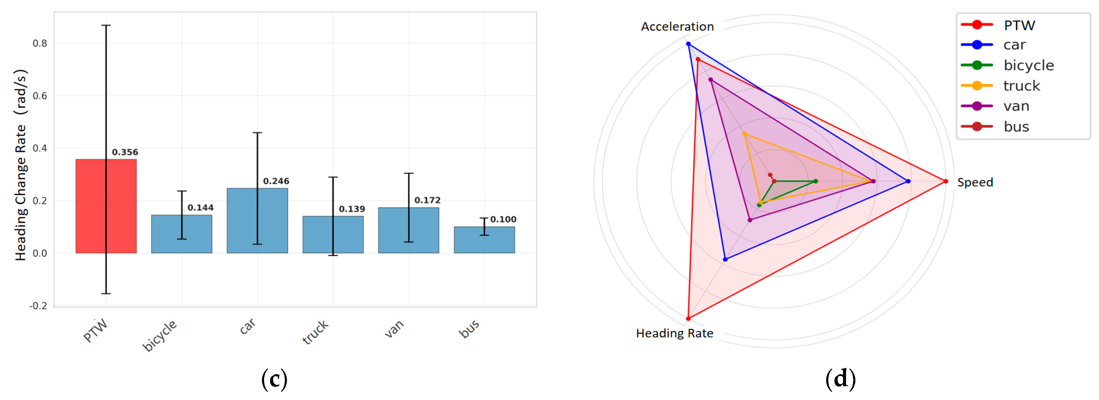
Analyzing the trajectory characteristics of PTWs is crucial for constructing the trajectory prediction model framework. This section selects trajectory data from the rounD dataset for feature analysis. The dataset provides high-precision spatiotemporal information, laying a foundation for the analysis of PTWs. Quantitatively revealing the unique trajectory characteristics in mixed traffic scenarios can provide an empirical basis for the design of trajectory prediction model components. The analysis involves the visualization and comparison of the average speed, average acceleration, and average heading change rate of various vehicle types within the studied scenario. This facilitates an intuitive analysis of the distinctive features of PTW trajectories. The detailed results are shown in Figure 1.
The analysis results presented in the figures clearly reveal the unique kinematic characteristics of powered two-wheelers (PTWs): The average speed of PTWs (7.92 m/s) is the highest among the analyzed vehicle types, significantly higher than that of bicycles (5.88 m/s) and even slightly surpassing that of cars (7.83 m/s) (Figure 1a). This indicates that PTWs typically maintain relatively high travel speeds within mixed traffic flow. In terms of acceleration, PTWs (1.50 m/s2) demonstrate strong acceleration capability, with a value second only to cars (1.58 m/s2) but considerably higher than bicycles, trucks, and buses (Figure 1b). This confirms the rapid start-up and braking capacity of PTWs resulting from their high power-to-weight ratio. The average heading change rate of PTWs (0.356 rad/s) is significantly higher than that of all other vehicle types (Figure 1c). This indicates more frequent and flexible directional adjustments during PTW movement, demonstrating high maneuverability and instability. The relatively large error bar also suggests significant variations in individual behaviors. The radar chart (Figure 1d) provides multidimensional corroboration of the above findings. The PTW profile covers the largest range on the acceleration and heading change rate axes, exhibiting a distinct and prominent shape that visually underscores its kinematic uniqueness and high dynamics. In contrast, cars excel in the speed dimension, while the indicators for other vehicle types are more concentrated.
Quantitative analysis of the trajectory characteristics indicates that relying solely on a single trajectory prediction framework and traditional interaction modeling perspectives is insufficient to characterize the significant features of PTWs, namely their high speed, high acceleration, and extremely high flexibility in heading changes. Therefore, it is necessary to treat motion features as an independent input channel, encoded by a dedicated LSTM branch. Simultaneously, a spatiotemporal attention mechanism is introduced to capture the key behavioral characteristics of PTWs from two dimensions, thereby improving the accuracy of trajectory prediction.

3.3. Model Architecture

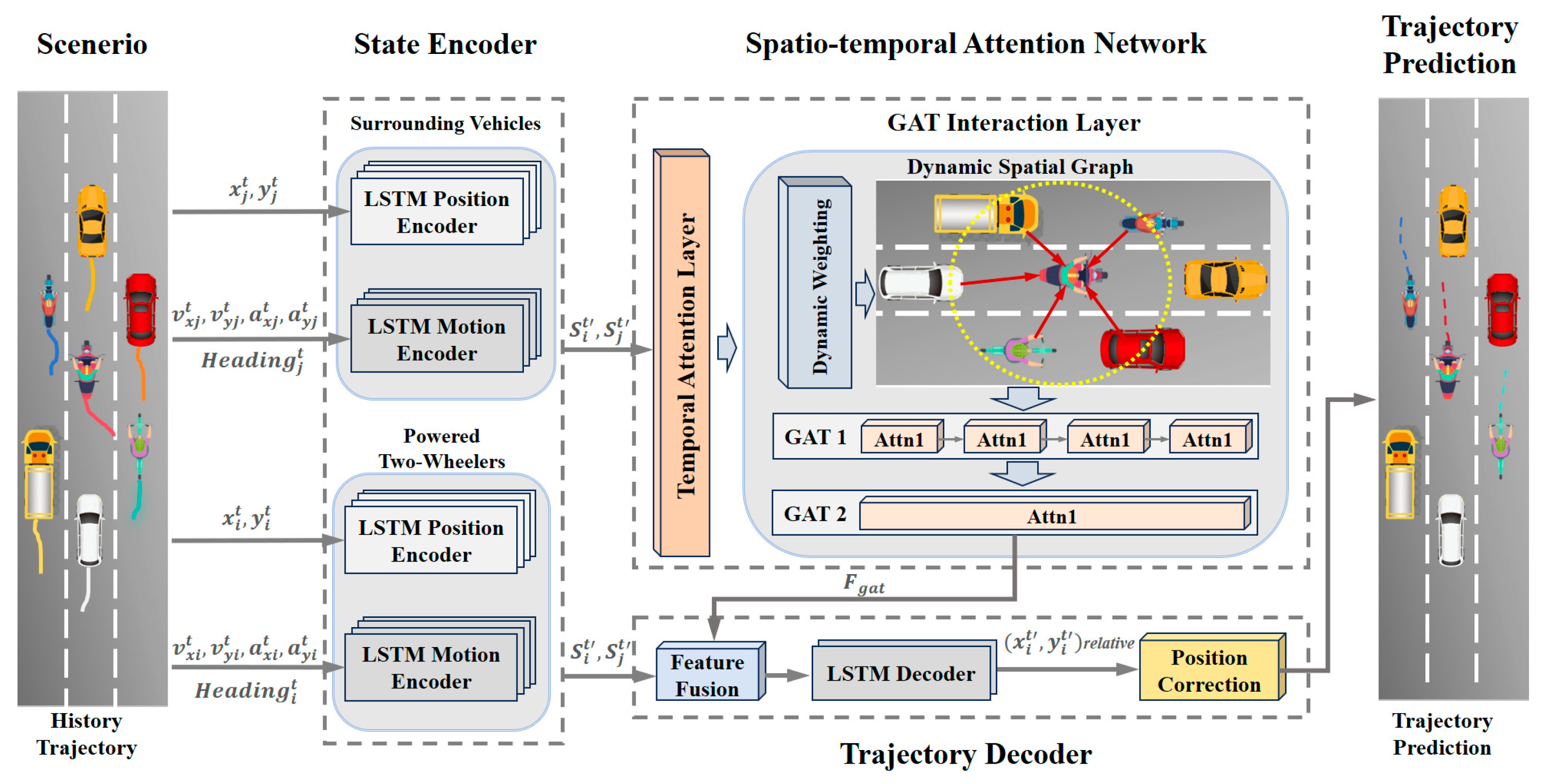
To address the limitations of existing research, we propose an enhanced LSTM encoder–decoder trajectory prediction framework integrated with graph attention, which deeply optimizes the complex motion characteristics of highly dynamic targets such as PTWs in mixed traffic scenarios. The model structure is shown in Figure 2. The model operates through three core modules working collaboratively: the trajectory feature encoding module separately encodes the positional and motion features of both PTWs and surrounding vehicles to effectively capture trajectory state characteristics; the spatiotemporal attention network module employs a temporal attention layer to extract features from key frames in the historical trajectory data, followed by a two-layer graph attention network to process interaction features between the target vehicle and surrounding traffic participants, ultimately outputting fused spatiotemporal features; and the decoder prediction module uses a two-layer LSTM to progressively generate future trajectories, which are further refined by a position correction module to improve the accuracy of the prediction results.

3.3.1. Trajectory State Encoder

Vehicle state information includes both positional state information and motion state information, which are fundamental elements constituting trajectories. Existing studies have shown that LSTM exhibits advantages in capturing sequential relationships in positional data and extracting critical features. Therefore, to precisely capture these two types of features while avoiding interference between the target vehicle’s characteristics and those of surrounding vehicles, this study adopts a separate encoding strategy for the target vehicle’s state features and the features of surrounding vehicles. Both encoder branches employ a dual-channel LSTM encoder strategy, dedicated to processing the positional sequences and motion features of vehicle trajectories, as detailed in Figure 2.
The LSTM position encoder receives the coordinate sequences of the historical trajectories of both the target vehicle and surrounding vehicles in the scene, and learns the spatial motion trends of vehicles through the LSTM network. To prevent overfitting during model training, the input to the position encoder consists of normalized relative position coordinates. After encoding by the position encoder module, the output includes the positional sequence features F pos , i t and F pos , j t for the target vehicle and surrounding vehicles, as shown in Formulas (1) and (2).
F pos , i t =   LSTM pos P i t   ,   F pos , i t 1  
F pos , j t = LSTM pos P j t   ,   F pos , j t 1  
The LSTM motion encoder receives multi-dimensional vectors of the PTW and surrounding vehicles, including velocity, acceleration, and heading angle, which reflect the instantaneous dynamic behaviors of vehicles in mixed traffic scenarios. After encoding by the motion encoder module, the output includes the motion features F mot , i t and F mot , j t for the target vehicle and surrounding vehicles, as shown in Formulas (3) and (4).
F mot , i t = LSTM mot V i t   ,   A i t ,   Heading i t , F mot , i t 1  
F mot , j t =   LSTM mot V j t   ,   A j t ,   Heading j t ,   F mot , j t 1  
It should be noted that in the state encoder module, the hidden layer dimension of the LSTM network is set to 128 for all branches, while the parameters of each encoder branch are trained independently to ensure precise capture of the most relevant features of different vehicles. Finally, the encoded trajectory features are concatenated to obtain the state features of the target vehicle and surrounding vehicles, denoted as F LSTM   =   ( S i t ,     S j t ) .

3.3.2. Spatiotemporal Attention Network

Temporal Attention Layer
The temporal attention module receives the hidden state feature sequence F LSTM R N × t h × 128 output by the LSTM state encoder, where N denotes the batch size. For the input feature sequence, the module first computes the mean vector S ave of the historical state sequence to extract global features, using the following formula:
S ave   =   1 t h t = 1 t h S t R N × 128
In Formula (5), S t denotes the LSTM hidden state sequences output by the LSTM state encoder at each historical time step.
Based on the above global feature processing, an importance scoring function (Formulas (6) and (7)) is further designed to compute the importance score A t for each time step, followed by normalization of the importance scores:
A t   =   W 2 tan h LayerNorm W 1 S t , S ave
α t = softmax A t
where α t represents the normalized importance score at each time step; W 1 R 128 × 128 denotes the learnable weight matrix of the first linear layer; and W 2 R 128 × 1 is the weight matrix of the second linear layer. Finally, the features of each time step are concatenated with the sequence average features, enabling the model to evaluate the deviation of the current moment from the overall behavior. The temporal context vector C R N × 1 × 128 is obtained through the Formula (8).
C = t = 1 t h α t S t
The temporal attention module incorporates a scene-adaptive attention mechanism that focuses on historical moments most influential to prediction. It specifically accounts for behavioral characteristics of motorcycles, such as sudden braking and frequent lane changes, and enhances the model’s responsiveness to abrupt behaviors through a dynamic weight allocation mechanism. This effectively addresses the “information dilution” issue faced by traditional LSTMs when processing long sequences.
GAT Interaction Layer
Interactions in mixed traffic scenarios exhibit characteristics of asymmetry and close-proximity dependency, with the interaction intensity between motorcycles and cars being significantly higher than that between cars. To address this, we designed a dual-layer residual graph attention network. Building upon the encoding of historical trajectory motion features, this architecture further employs a spatial attention mechanism to dynamically capture social dependencies, with particular focus on the interaction patterns of motorcycles within dense traffic flow.
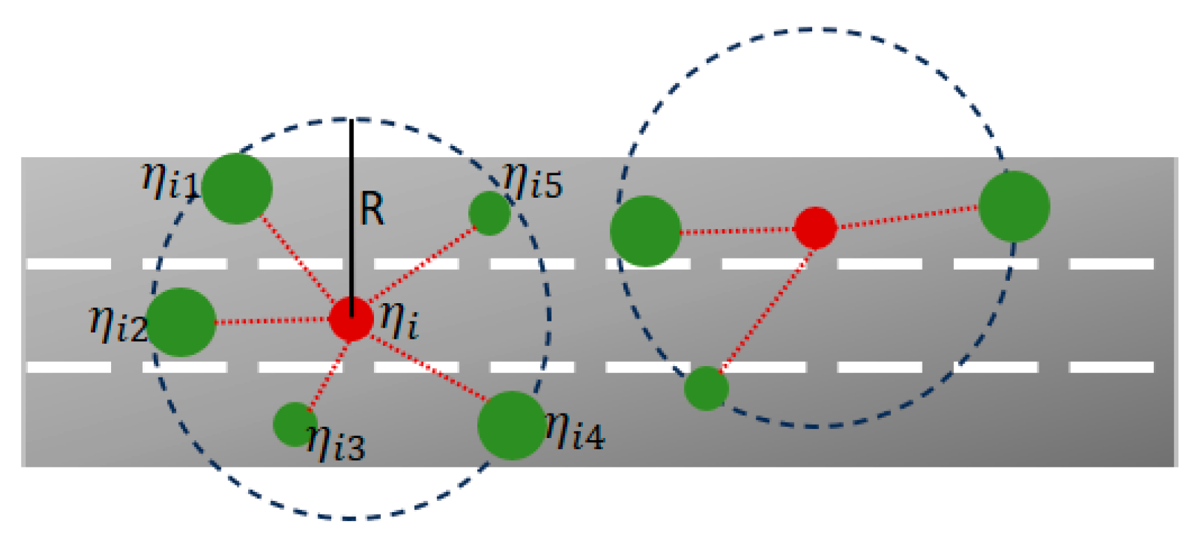
The GAT module receives the state feature sequences of both the target vehicle and surrounding vehicles, processed by the LSTM encoder and the temporal attention module, as node features. The set of adjacent nodes for MTW i is denoted as η i = η i 1 ,   η i 2 ,   η i 3   η ij , where each node represents a traffic participant. Edges represent interaction relationships between nodes, which are determined by computing the Euclidean distance matrix D i , j (Formula (9)) to construct the dynamic interaction graph.
D i , j =   1 , i f   P i P j 2   R   0 , o t h e r w i s e  
where P i P j 2 denotes the Euclidean distance between two interacting vehicles, and its calculation method is shown in Formula (10):
P i P j 2 = x i x j 2 + y i y j 2
Meanwhile, this study refers to existing research [42] for setting the interaction radius threshold R. Considering the maneuvering characteristics of PTWs in mixed traffic scenarios, pre-experimental validation revealed that setting the interaction radius threshold R to 5 m for PTWs yielded the best prediction performance of the model. That is, the model most comprehensively and meticulously captures the interactive behavioral features of vehicles within a 5 m radius of the target vehicle. Constructing the dynamic graph using this criterion ensures optimal model performance. It is noteworthy that this study assumes the influence of surrounding vehicles outside the interaction radius at a given moment can be negligible for the target vehicle at that moment. The constructed dynamic graph is shown in Figure 3.
The first layer of the dual-layer residual graph attention network employs a multi-head attention mechanism (4 heads), where each head learns independent attention weights, enhancing the model’s capability to capture diverse interaction patterns. The first GAT layer learns the interactive features between the target vehicle and surrounding vehicles within the interaction radius by processing the historical position sequence features of the surrounding vehicles F pos , j t . The output feature F gat 1 is calculated as shown in Formula (11):
F gat 1   =   | | n = 1 4 σ j η i α ij n W n F pos , j
where | | denotes the feature concatenation operation, enhancing feature diversity; σ is a nonlinear activation function that improves the model’s capacity to represent complex interaction patterns; W n represents the learnable weight matrix of the n-th attention head, projecting the 128-dimensional positional features into a 64-dimensional interaction space; and α ij n is the normalized attention coefficient of node i to node j in the n-th head. The value of is related to the vehicle type, motion features, and the Euclidean distance to the target vehicle. Its magnitude directly indicates the relative importance of the influence of that neighboring vehicle on the target vehicle. Their calculation formula is shown in Formula (12).
α ij n = softmax a T W n F pos , i     W n F pos , j
In Formula (12), a is a learnable attention parameter vector used to control the importance of interaction features in weight computation, which is automatically optimized through backpropagation.
The second layer of the two-layer residual graph attention network aggregates multi-head features through a single-head attention mechanism and outputs 64-dimensional interaction features F gat 2 , calculated as shown in Formula (13):
F gat 2 = σ j η i β ij V F gat 1 , j
where V is a learnable projection matrix that compresses F gat 1 R N × t h × 256 into a 64-dimensional unified space; F gat 1 , j denotes the first-layer interaction feature output for a specific vehicle j . β ij represents the normalized attention weight, calculated as shown in Formula (14), where q in the formula denotes a learnable query vector.
β ij = softmax q T W n F pos , i     W n F gat 1 , j
A residual connection is subsequently introduced to enable the model to retain the vehicle’s own motion features without being overwhelmed by interaction features, as shown in Formula (15). Here, F pos denotes the positional features output by the temporal attention layer.
F gat =   F gat 2 + Linear 128 64 F pos

3.3.3. Trajectory Decoder

The decoding and prediction module is responsible for converting the encoded and fused spatiotemporal features into future trajectory predictions. This module consists of three processing stages: feature fusion, LSTM decoding, and absolute position correction.
First, the feature fusion module receives the state features F LSTM output by the LSTM encoder module and the interaction features F gat output by the spatiotemporal attention module. These features are fused along the feature dimension to form a fused feature matrix, as described in Formula (16).
F fusion =   F LSTM     F gat , F fusion   R N × t h × ( 128 + 64 )
The fused feature matrix F fusion is fed into a two-layer LSTM decoder to decode the integrated features. The first LSTM layer processes the spatiotemporal–social mixed features and outputs intermediate states; the second LSTM layer further extracts temporal dependencies, as described in Formula (17).
f dec     t ,     c dec   t =   LSTM dec F fusion   t   ,   f dec   t 1 ,   c dec   t 1
where the hidden state f dec     t   R 128 and the cell state   c dec   t   R 128 at each time step are passed to the next time step, enabling cross-temporal information memory.
Subsequently, the output of the two-layer LSTM decoder is transformed into relative displacement predictions through an MLP nonlinear layer, as shown in Formula (18).
Δ P ^ i t = W 0 · ReLU LayerNorm W 3 · f dec t + b 0 + b 1
where Δ P ^ i   t represents the predicted relative displacement of PTW i at time t ; W 0   R 64 × 2 and W 3   R 128 × 64 are learnable parameters of the fully connected layers, mapping features from high-dimensional to low-dimensional spaces; b 0   R 64 and b 1   R 2 denote the biases of the first fully connected layer and the output layer, respectively.
Finally, to mitigate the impact of starting point drift on trajectory prediction accuracy, an absolute position correction method is introduced. Using the true position coordinates   P i t 1 at the last observed time point as the reference, the predicted relative displacement Δ P ^ i   t output by the decoder is converted into absolute position coordinates P ^ i t , as calculated in Formula (19).
P ^ i t = Δ P ^ i t + P i t 1
After a series of decoding and position correction operations, the final output is the trajectory of the PTW within the prediction horizon.

4. Experiments and Analysis

To validate the effectiveness of the proposed PTW trajectory prediction model, experiments are conducted on the rounD trajectory dataset. Subsequently, three evaluation metrics—Average Displacement Error (ADE), Final Displacement Error (FDE), and Root Mean Square Error (RMSE)—are selected to assess the performance of the trajectory prediction model. The results are compared with various models from recent research in the field to demonstrate the superior performance of the proposed model. Meanwhile, ablation studies are designed to investigate the impact of each module on the model’s performance. Finally, a visual analysis is performed on the prediction outputs from each experiment.

4.1. Dataset

This study validates the model on the rounD trajectory dataset [43], which was released by the Institute for Automotive Engineering at RWTH Aachen University, Germany. The team collected data using drones equipped with cameras and employed advanced computer vision algorithms to ensure high positioning accuracy, effectively overcoming common challenges such as occlusion inherent in traditional traffic data collection methods. In terms of vehicle trajectory processing, the rounD dataset utilizes an advanced high-resolution semantic segmentation network (DeepLab-v3+) to process 4K aerial footage, generating polygonal contours for each road user (Figure 4a,b). The centroid of each vehicle’s bounding box is then calculated and used as the positional coordinates for various vehicle types. This approach represents a standard practice in the fields of computer vision and trajectory analysis, providing a unified and unambiguous reference point for vehicles of different geometric shapes (such as long trucks and compact motorcycles), thereby avoiding the ambiguity associated with using position points like the front or rear of vehicles that vary with their orientation. The dataset, published in 2020, records trajectory data of natural road users at three different roundabouts in Germany, as shown in Figure 4c. It includes over 13,746 road users and 6 h of trajectory information, covering cars, vans, trucks, buses, pedestrians, bicycles, and motorcycles. The sampling rate of the dataset is 25 Hz.

4.2. Evaluation Metrics and Implementation Details

With reference to existing research achievements in trajectory prediction, this study selects three commonly used evaluation metrics—ADE, FDE, and RMSE—to assess the performance of the trajectory prediction model. The formulas are as follows:
ADE = 1 N i = 1 N 1 T t = 1 T P ^ i t P i t 2
FDE = 1 N i = 1 N P ^ i T P i T 2
RMSE t = 1 N i = 1 N P ^ i t P i t 2
among these, ADE is the mean squared error between the true and predicted positions of trajectory points over 50 time steps (2 s); FDE refers to the Euclidean distance between the predicted and true values of the final position in the target vehicle’s trajectory;   RMSE t represents the root mean square error between the predicted trajectory and the ground truth trajectory at specific time points t   =   [ 10 ,     20 ,     30 ,     40 ,     50 ] .
The experiments in this study were implemented in an Ubuntu 20.04 environment using CUDA 11.8, Python 3.8, and PyTorch 2.0.0. An RTX 4090D GPU with 80 GB of memory was used for execution. During training, the Adam optimizer was selected to minimize the loss function. Additionally, the batch size was set to 128, the number of epochs to 100, the dropout rate to 0.2, and the minimum learning rate to 1 × 10⁻⁵. Under the aforementioned hardware environment, the model achieves a single-trajectory prediction latency of 11.62 milliseconds, attaining a safety margin of 88%. This performance significantly outperforms the real-time threshold required by autonomous driving systems, enabling efficient handling of real-time prediction tasks in complex interactive scenarios. Furthermore, the model maintains a compact parameter size of 0.61 M with a computational complexity of 0.08 GFLOPs. These results demonstrate that the structurally efficient trajectory prediction framework developed in this study effectively reduces computational overhead while fulfilling the stringent real-time requirements of practical applications, thereby providing a robust technical foundation for its integration into autonomous driving systems.
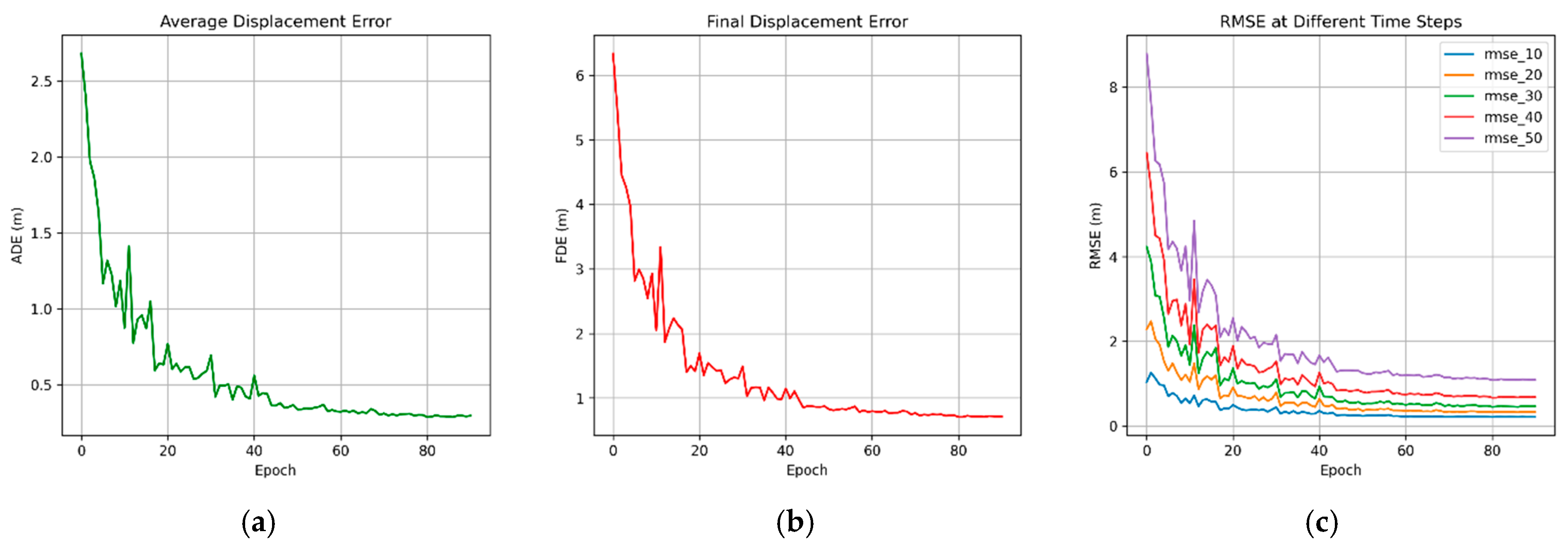
As shown in Figure 5, all metrics gradually stabilize during the training process and decrease to a low level, indicating that the proposed model performs well in the trajectory prediction task on this dataset and achieves high-precision prediction of PTW trajectories in mixed traffic scenarios.
The loss function of the proposed model adopts a composite multi-objective design, combining three key metrics: ADE, Start-point Alignment Penalty (SE), and Maximum Displacement Error (MDE) constraint (Formula (23)).
L = λ 1 · ADE   +   λ 2 · SE   +   λ 3 · MDE
Among these, the calculation formulas for SE and MDE in Formula (23) are given by Formula (24) and Formula (25), respectively.
SE = P ^ i 0 P i 0 2
MDE = max P ^ i t P i t 2
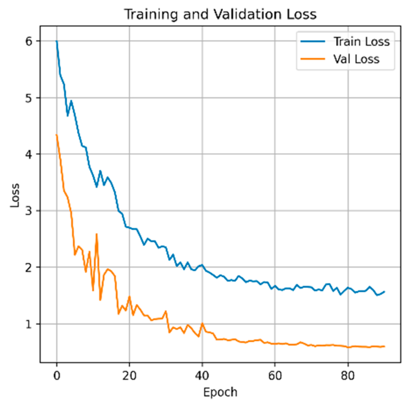
P ^ i 0 and P i 0 represent the predicted trajectory coordinates and the true trajectory coordinates of PTW i at the initial prediction time step t pred   =   0 , respectively; λ 1 ,   λ 2 ,   λ 3 are the weight coefficients for the three metrics. Figure 6 shows the training and validation loss curve in the mixed traffic scenario where the dataset is located.
The design of the loss function ensures the overall accuracy of the trajectory shape while specifically enhancing the motion continuity at the trajectory start point, and improves the model’s robustness to extreme cases by penalizing the maximum deviation term. As shown in Figure 6, both the training loss curve and the validation loss curve stabilize by the end of the training process, demonstrating the effectiveness of the loss function.

4.3. Model Comparison Experimental Results and Analysis

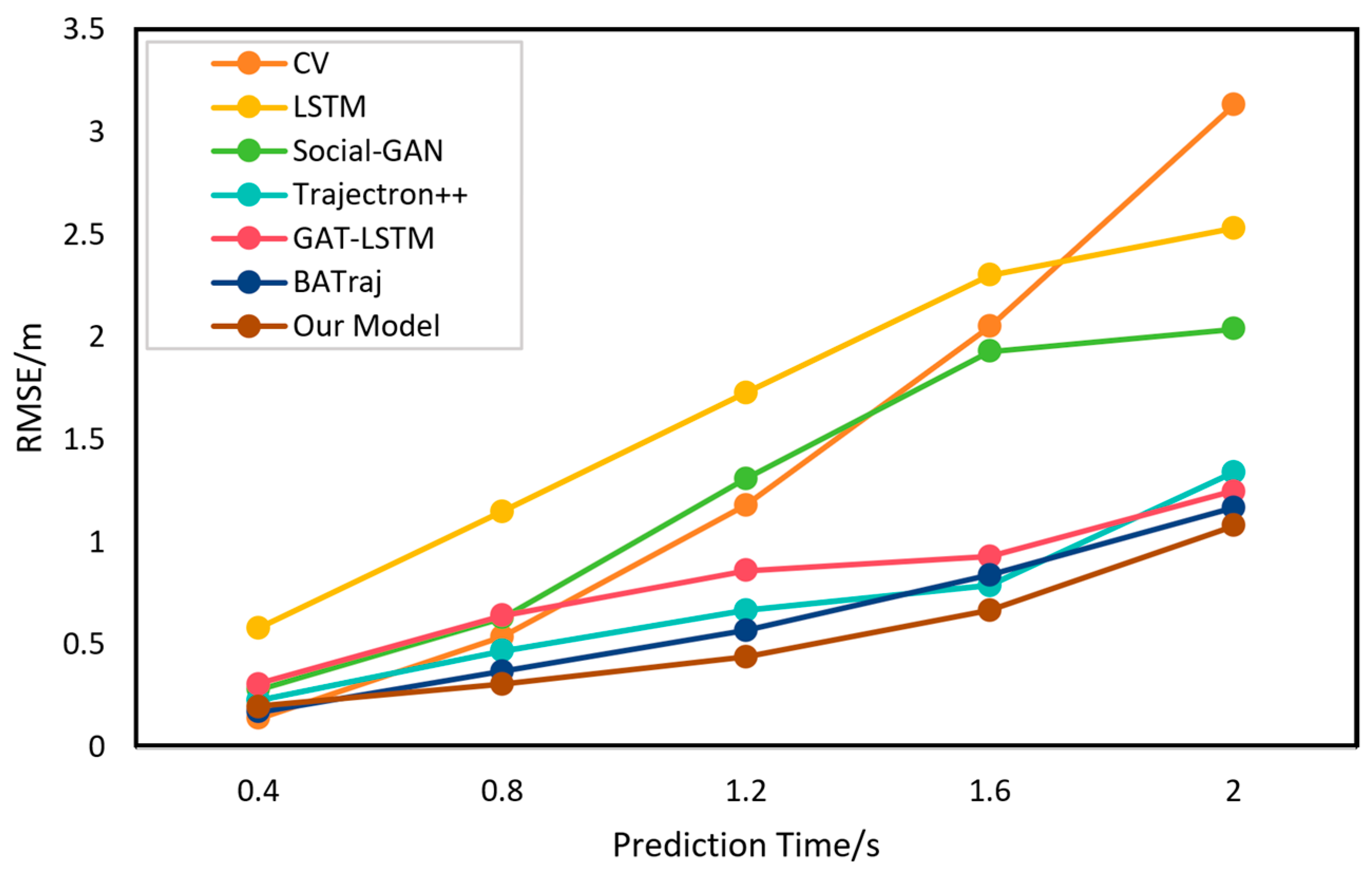
To validate the trajectory prediction performance of the proposed model for PTWs in mixed traffic scenarios, we selected six recently proposed models for comparative experiments on the rounD dataset. It should be noted that all models take the 2 s historical trajectory of the target vehicle as input and output the predicted trajectory of the target vehicle for the next 2 s in the scenario. The experimental results are shown in Table 2 and Figure 7. It should be noted that in Table 2, the underlined values indicate the parameters obtained from the validation of the best-performing model under the respective conditions, while the bolded values represent the verification results of the model proposed in this study.
CV [10]: This method assumes that objects continue moving at their current speed and direction, while ignoring interactions between vehicles. Trajectory prediction is performed based on these assumptions.
LSTM [44]: It employs an LSTM encoder–decoder framework, taking only the coordinates of the target as input and outputting trajectory predictions.
Social-GAN [45]: This model improves upon Social-LSTM by introducing a generative adversarial learning mechanism to achieve vehicle trajectory prediction in highly interactive scenarios.
Trajectron++ [42]: It captures complex spatiotemporal dependencies via GNNs, utilizes CAVE to handle uncertainty in agent intentions and generate diverse trajectories, and incorporates kinematic and dynamic models to ensure the feasibility of output trajectories.
GAT-LSTM [46]: It uses LSTM networks to encode vehicle trajectory information and employs GAT to represent vehicle interactions, fully considering the dynamics and spatiotemporal correlations of multidimensional motion.
BATraj [47]: This approach captures continuous driving behavior using only historical trajectory data in polar coordinates and a DGG-based method, eliminating the need for labor-intensive HD maps and costly manual annotations.
The comparative experimental results on the rounD dataset fully demonstrate the significant advantages of the proposed model in mixed traffic scenarios. As shown in Table 2 and Figure 7, our model achieves optimal or near-optimal performance across multiple key metrics. At a 0.8s prediction horizon, it attains the lowest RMSE of 0.31, representing a 16.2% reduction compared to the second-best performer, BATraj (0.37). At 1.2 s, the RMSE is 0.44, significantly outperforming Social-GAN (1.31) and GAT-LSTM (0.86). Most notably, our model achieves an outstanding ADE of 0.28, surpassing all baseline models—9.68% lower than Trajectron++ (0.31) and 69.2% lower than Social-GAN (0.91). Although its FDE of 0.70 is slightly higher than BATraj’s 0.67, when considering the overall performance in ADE and RMSE across time periods, our model exhibits clear superiority in both the accuracy and stability of trajectory prediction. It maintains a leading position, especially in the short-to-medium term prediction range (0.4 s to 1.6 s), which indicates that the proposed model more sensitively captures the highly dynamic and interactive behaviors of PTWs in mixed traffic scenarios, enabling trajectory predictions to converge stably closer to the ground truth. This further enhances the operational safety of autonomous driving systems in such environments.

4.4. Ablation Experimental Results and Analysis

The model framework proposed in this study consists of four main modules: LSTM encoder, temporal attention module, graph attention module, and trajectory decoder. To systematically investigate the specific contributions of different module components in improving the model’s performance, we conducted a series of ablation experiments. Six model variants were compared and quantitatively evaluated using both ADE and FDE metrics, as shown in Table 3. It should be noted that in the table, “×” indicates that the module was removed from the model, while “√” indicates that the module was retained. Additionally, underlined values represent the verification results of the best-performing model under the respective conditions, and bolded values denote the verification results of the complete model proposed in this study.
Experimental results demonstrate that the complete model achieved the best performance, with ADE and FDE reaching 0.28 m and 0.70 m, respectively, significantly surpassing all other ablation configurations, which verifies the effectiveness of each module’s design and their positive contribution to the overall prediction performance.
Data from the table show that removing the temporal attention layer led to a decline in model performance, with ADE and FDE reaching 0.36 m and 0.83 m, respectively. This indicates that the module plays an indispensable role in enhancing the model’s perception of dynamic features at critical time steps. Furthermore, when the graph attention interaction layer (GAT) was removed, ADE and FDE increased to 0.53 m and 0.95 m, respectively, indicating considerable performance degradation. This underscores the critical importance of explicitly modeling spatial relationships among agents for accurate future trajectory prediction. The removal of the feature fusion module resulted in a substantial increase in ADE, while FDE also rose to 0.86 m, demonstrating that this module plays a central role in integrating multi-source feature information. Similarly, when the position correction module was excluded, ADE and FDE reached 0.48 m and 0.88 m, respectively, indicating that this module effectively enhances the spatial consistency and physical plausibility of trajectories and substantially contributes to improving the accuracy of decoded trajectories.
We also tested a model with both the temporal attention and graph attention modules removed simultaneously, which resulted in the worst performance, with ADE and FDE as high as 0.65 m and 1.23 m, respectively, significantly exceeding all other ablation settings. This indicates that both temporal and spatial modeling modules constitute the core capability of the model, and neither can be omitted. Finally, under the configuration where both the feature fusion and position correction modules were omitted, the evaluated ADE and FDE values showed a noticeable increase. Although the magnitude of degradation was less severe than in the previous ablation experiment, the overall prediction consistency—particularly the final displacement error—was still affected, demonstrating the necessity of multi-module collaboration.

5. Conclusions

This paper addresses the challenge of predicting powered two-wheeler (PTW) trajectories in mixed traffic scenarios by proposing an enhanced Social-GAT prediction model. The core innovation of this research lies in constructing a multi-module collaborative architecture specifically designed for PTW characteristics: A dual-channel LSTM encoder separately processes positional sequences and motion features to effectively capture the high maneuverability of PTWs; a temporal attention mechanism is introduced to enhance the perception of key behavioral moments; and a residual-connected dual-layer GAT structure is employed for fine-grained modeling of asymmetric interactions between PTWs and vehicles. Experiments on the rounD dataset demonstrate that the proposed model significantly outperforms baseline models in PTW trajectory prediction tasks, with ablation studies further validating the contribution of each module. Notably, the removal of the GAT layer led to a significant performance degradation, underscoring the necessity of a dedicated interaction modeling mechanism in the model.
The model proposed in this study provides key technical support for the safety decision-making of autonomous driving systems in mixed traffic environments. Its high-precision prediction capability offers a longer reaction time for the path planning module of autonomous vehicles, effectively reducing collision risks in complex scenarios such as intersections and ramps. Furthermore, based on feature learning, it can generate trajectory data that conforms to the real behavioral characteristics of PTWs, providing a high-quality simulation benchmark for the testing and validation of autonomous driving algorithms.
However, due to the limited PTW samples in currently available public datasets and the variations in traffic contexts across different countries and regions, training on a single dataset still struggles to fully capture important behavioral features in interactive scenarios. In future work, we will incorporate transfer learning methods to validate the model on more datasets, overcoming trajectory prediction accuracy issues caused by small sample sizes and data distribution disparities. The focus will be on exploring the model’s generalization capability across regions and scenarios, further enhancing the practicality and reliability of trajectory prediction models in complex interactive environments.

Author Contributions

Writing—original draft preparation and writing—review and editing, L.Z.; supervision and project administration, F.C.; data curation, J.L. and H.W.; supervision and funding acquisition, Y.L. and Z.Z. All authors have read and agreed to the published version of the manuscript.

Funding

This research was funded by the Guangxi Science and Technology Major Project (Grant No. AA22068057) and the National Natural Science Foundation of China (Grant Nos. 62262009, 62495083).

Data Availability Statement

The data are available upon reasonable request.

Acknowledgments

The authors are grateful to the editors and the anonymous reviewers for their insightful comments and suggestions.

Conflicts of Interest

The authors declare that they have no known competing financial interests or personal relationships that could have influenced the work reported in this paper.

References

  1. Huang, Y.; Du, J.; Yang, Z.; Zhou, Z.; Zhang, L.; Chen, H. A survey on trajectory-prediction methods for autonomous driving. IEEE Trans. Intell. Veh. 2022, 7, 652–674. [Google Scholar] [CrossRef]
  2. Liu, Q.; Sun, J.; Tian, Y.; Ni, Y.; Yu, S. Modeling and simulation of nonmotorized vehicles’ dispersion at mixed flow intersections. J. Adv. Transp. 2019, 2019, 9127062. [Google Scholar] [CrossRef]
  3. Li, J.; Ni, Y.; Sun, J. A Two-layer integrated model for cyclist trajectory prediction considering multiple interactions with the environment. Transp. Res. Part C Emerg. Technol. 2023, 155, 104304. [Google Scholar] [CrossRef]
  4. Maurer, L.F.; Meister, A.; Axhausen, K.W. Cycling speed profiles from GPS data: Insights for conventional and electrified bicycles in Switzerland. J. Cycl. Micromobil. Res. 2025, 5, 100077. [Google Scholar] [CrossRef]
  5. Hochreiter, S.; Schmidhuber, J. Long short-term memory. Neural Comput. 1997, 9, 1735–1780. [Google Scholar] [CrossRef]
  6. Scarselli, F.; Gori, M.; Tsoi, A.C.; Hagenbuchner, M.; Monfardini, G. The graph neural network model. IEEE Trans. Neural Netw. 2009, 20, 61–80. [Google Scholar] [CrossRef]
  7. Li, J.; Yang, L.; Chen, Y.; Jin, Y. MFAN: Mixing feature attention network for trajectory prediction. Pattern Recognit. 2024, 146, 109997. [Google Scholar] [CrossRef]
  8. Yan, Y.; Zhang, B.; Li, C. A networked multi-agent reinforcement learning approach for cooperative FemtoCaching assisted wireless heterogeneous networks. Comput. Netw. 2023, 220, 109513. [Google Scholar] [CrossRef]
  9. Leigh, A.; Pineau, J.; Olmedo, N.; Zhang, H. Person tracking and following with 2D laser scanners. In Proceedings of the International Conference on Robotics and Automation, Seattle, WA, USA, 26–30 May 2015; pp. 726–733. [Google Scholar] [CrossRef]
  10. Schöller, C.; Aravantinos, V.; Lay, F.; Knoll, A. What the constant velocity model can teach us about pedestrian motion prediction. IEEE Robot. Autom. Lett. 2020, 5, 1696–1703. [Google Scholar] [CrossRef]
  11. Liu, K.; Wang, W.; Gong, J. Dynamic modeling and trajectory tracking of intelligent vehicles in off-road terrain. J. Beijing Inst. Technol. 2019, 39, 933–937. [Google Scholar] [CrossRef]
  12. Liao, J.H. Research on LiDAR/IMU Integrated Navigation and Positioning Method. Ph.D. Theis, Nanchang University, Nanchang, China, 6 June 2020. [Google Scholar] [CrossRef]
  13. Lefkopoulos, V.; Menner, M.; Domahidi, A.; Zeilinger, M.N. Interaction-aware motion prediction for autonomous driving: A multiple model Kalman filtering scheme. IEEE Robot. Autom. Lett. 2020, 6, 80–87. [Google Scholar] [CrossRef]
  14. Li, X.; Rosman, G.; Gilitschenski, I.; Vasile, C.I.; DeCastro, J.A.; Karaman, S.; Rus, D. Vehicle trajectory prediction using generative adversarial network with temporal logic syntax tree features. IEEE Robot. Autom. Lett. 2021, 6, 3459–3466. [Google Scholar] [CrossRef]
  15. Zhang, S.; Zhi, Y.; He, R.; Li, J. Research on traffic vehicle behavior prediction method based on game theory and HMM. IEEE Access 2020, 8, 30210–30222. [Google Scholar] [CrossRef]
  16. Huang, L.; Wu, J.; You, F.; Lv, Z.; Song, H. Cyclist social force model at unsignalized intersections with heterogeneous traffic. IEEE Trans. Ind. Inform. 2017, 13, 782–792. [Google Scholar] [CrossRef]
  17. Yan, Z.; Yue, L.; Sun, J. High-resolution reconstruction of non-motorized trajectory in shared space: A new approach integrating the social force model and particle filtering. Expert Syst. Appl. 2023, 233, 120753. [Google Scholar] [CrossRef]
  18. Huang, Z.; Wang, J.; Pi, L.; Song, X.; Yang, L. LSTM based trajectory prediction model for cyclist utilizing multiple interactions with environment. Pattern Recognit. 2021, 112, 107800. [Google Scholar] [CrossRef]
  19. Rong, H.; Teixeira, A.P.; Soares, C.G. Ship trajectory uncertainty prediction based on a Gaussian process model. Ocean Eng. 2019, 182, 499–511. [Google Scholar] [CrossRef]
  20. Mandalia, H.; Salvucci, D. Using support vector machines for lane-change detection. In Proceedings of the Human Factors and Ergonomics Society Annual Meeting, Orlando, FL, USA, 26–30 September 2005; Volume 49, pp. 1965–1969. [Google Scholar] [CrossRef]
  21. He, G.; Li, X.; Lv, Y.; Gao, B.; Chen, H. Probabilistic intention prediction and trajectory generation based on dynamic Bayesian networks. In Proceedings of the 2019 Chinese Automation Congress (CAC), Hangzhou, China, 22–24 November 2019; pp. 2646–2651. [Google Scholar] [CrossRef]
  22. Yang, J.; Liu, J. Vehicle trajectory prediction model based on graph attention Kolmogorov-Arnold networks and multiple attention. Eng. Appl. Artif. Intell. 2025, 159, 111804. [Google Scholar] [CrossRef]
  23. Chung, J.; Gulcehre, C.; Cho, K.; Bengio, Y. Empirical evaluation of gated recurrent neural networks on sequence modeling. arXiv 2014, arXiv:1412.3555. [Google Scholar] [CrossRef]
  24. Li, T.; Sun, X.; Dong, Q.; Guo, G. DSTAnet: A trajectory distribution-aware spatio-temporal attention network for vehicle trajectory prediction. IEEE Trans. Veh. Technol. 2025, 74, 10187–10197. [Google Scholar] [CrossRef]
  25. Pool, E.A.I.; Kooij, J.F.P.; Gavrila, D.M. Context-based cyclist path prediction using recurrent neural networks. In Proceedings of the IEEE Intelligent Vehicles Symposium (IV), Paris, France, 9–12 June 2019; pp. 824–830. [Google Scholar] [CrossRef]
  26. Scheel, O.; Nagaraja, N.S.; Schwarz, L.; Navab, N.; Tombari, F. Attention-based lane change prediction. In Proceedings of the International Conference on Robotics and Automation, Montreal, QC, Canada, 20–24 May 2019; pp. 8655–8661. [Google Scholar] [CrossRef]
  27. Sun, J.; Qi, X.; Xu, Y.; Tian, Y. Vehicle turning behavior modeling at conflicting areas of mixed-flow intersections based on deep learning. IEEE Trans. Intell. Transp. Syst. 2020, 21, 3674–3685. [Google Scholar] [CrossRef]
  28. Peng, Y.; Zhang, G.; Shi, J.; Xu, B.; Zheng, L. SRAI-LSTM: A social relation attention-based interaction-aware LSTM for human trajectory prediction. Neurocomputing 2022, 490, 258–268. [Google Scholar] [CrossRef]
  29. Helbing, D.; Molnár, P. Social force model for pedestrian dynamics. Phys. Rev. E 1995, 51, 4282. [Google Scholar] [CrossRef]
  30. Alahi, A.; Goel, K.; Ramanathan, V.; Robicquet, A.; Li, F.F.; Savarese, S. Social LSTM: Human trajectory prediction in crowded spaces. In Proceedings of the IEEE/CVF Conference on Computer Vision and Pattern Recognition, Las Vegas, NV, USA, 27–30 June 2016; pp. 961–971. [Google Scholar] [CrossRef]
  31. Chandra, R.; Bhattacharya, U.; Bera, A.; Manocha, D. TraPHic: Trajectory prediction in dense and heterogeneous traffic using weighted interactions. In Proceedings of the IEEE/CVF Conference on Computer Vision and Pattern Recognition, Long Beach, CA, USA, 15–20 June 2019; pp. 8483–8492. [Google Scholar] [CrossRef]
  32. Jia, X.; Wu, P.; Chen, L.; Liu, Y.; Li, H.; Yan, J. HDGT: Heterogeneous driving graph transformer for multi-agent trajectory prediction via scene encoding. IEEE Trans. Pattern Anal. Mach. Intell. 2023, 45, 13860–13875. [Google Scholar] [CrossRef]
  33. Velickovic, P.; Cucurull, G.; Casanova, A.; Romero, A.; Lio, P.; Bengio, Y. Graph attention networks. arXiv 2017, arXiv:1710.10903. [Google Scholar] [CrossRef]
  34. Zhou, Z.; Ye, L.; Wang, J.; Wu, K.; Lu, K. HiVT: Hierarchical vector transformer for multi-agent motion prediction. In Proceedings of the IEEE/CVF Conference on Computer Vision and Pattern Recognition, New Orleans, LA, USA, 18–24 June 2022; pp. 8813–8823. [Google Scholar] [CrossRef]
  35. Li, Q.; Ou, B.; Liang, Y.; Wang, Y.; Yang, X.; Li, L. TCN-SA: A Social attention network based on temporal convolutional network for vehicle trajectory prediction. J. Adv. Transp. 2023, 2023, 1286977. [Google Scholar] [CrossRef]
  36. Zhan, T.; Zhang, Q.; Chen, G.; Cheng, J. VRR-Net: Learning vehicle-road relationships for vehicle trajectory prediction on highways. Mathematics 2023, 11, 1293. [Google Scholar] [CrossRef]
  37. Li, R.; Qin, Y.; Wang, J.; Wang, H. AMGB: Trajectory prediction using attention-based mechanism GCN-BiLSTM in IOV. Pattern Recognit. Lett. 2023, 169, 17–27. [Google Scholar] [CrossRef]
  38. Zheng, X.; Chen, X.; Jia, Y. Vehicle trajectory prediction based on GAT and LSTM networks in urban environments. Promet-Traffic Transp. 2024, 36, 867–884. [Google Scholar] [CrossRef]
  39. Zhang, J.; Guo, L.; Wang, G.; Yu, J.; Zheng, X.; Mei, Y.; Han, B. A dual-level graph attention network and transformer for enhanced trajectory prediction under road network constraints. Expert Syst. Appl. 2025, 261, 125510. [Google Scholar] [CrossRef]
  40. Shi, S.; Jiang, L.; Dai, D.; Schiele, B. MTR++: Multi-agent motion prediction with symmetric scene modeling and guided intention querying. IEEE Trans. Pattern Anal. Mach. Intell. 2024, 46, 3955–3971. [Google Scholar] [CrossRef] [PubMed]
  41. Jo, E.; Sunwoo, M.; Lee, M. Vehicle trajectory prediction using hierarchical graph neural network for considering interaction among multimodal maneuvers. Sensors 2021, 21, 5354. [Google Scholar] [CrossRef] [PubMed]
  42. Salzmann, T. Trajectron++: Dynamically-feasible trajectory forecasting with heterogeneous data. In Proceedings of the European Conference on Computer Vision, Glasgow, UK, 23–28 August 2020; pp. 683–700. [Google Scholar] [CrossRef]
  43. Krajewski, R.; Moers, T.; Bock, J.; Vater, L.; Eckstein, L. The round dataset: A drone dataset of road user trajectories at roundabouts in Germany. In Proceedings of the 2020 IEEE 23rd International Conference on Intelligent Transportation Systems (ITSC), Rhodes, Greece, 20–23 September 2020; pp. 1–6. [Google Scholar] [CrossRef]
  44. Saleh, K.; Hossny, M.; Nahavandi, S. Cyclist trajectory prediction using bidirectional recurrent neural networks. In Proceedings of the Australasian Joint Conference on Artificial Intelligence, Wellington, New Zealand, 11–14 December 2018; Volume 11320, pp. 284–295. [Google Scholar] [CrossRef]
  45. Gupta, A.; Johnson, J.; Li, F.F.; Savarese, S.; Alahi, A. Social GAN: Socially acceptable trajectories with generative adversarial networks. In Proceedings of the IEEE Conference on Computer Vision and Pattern Recognition, Salt Lake City, UT, USA, 18–22 June 2018; pp. 2255–2264. [Google Scholar] [CrossRef]
  46. Wang, J.; Liu, K.; Li, H. LSTM-based graph attention network for vehicle trajectory prediction. Comput. Netw. 2024, 248, 110477. [Google Scholar] [CrossRef]
  47. Liao, H.; Li, Z.; Shen, H.; Zeng, W.; Liao, D.; Li, G.; Xu, C. BAT: Behavior-aware human-like trajectory prediction for autonomous driving. In Proceedings of the AAAI Conference on Artificial Intelligence, Philadelphia, PA, USA, 25 February–4 March 2024; Volume 38, pp. 10332–10340. [Google Scholar] [CrossRef]
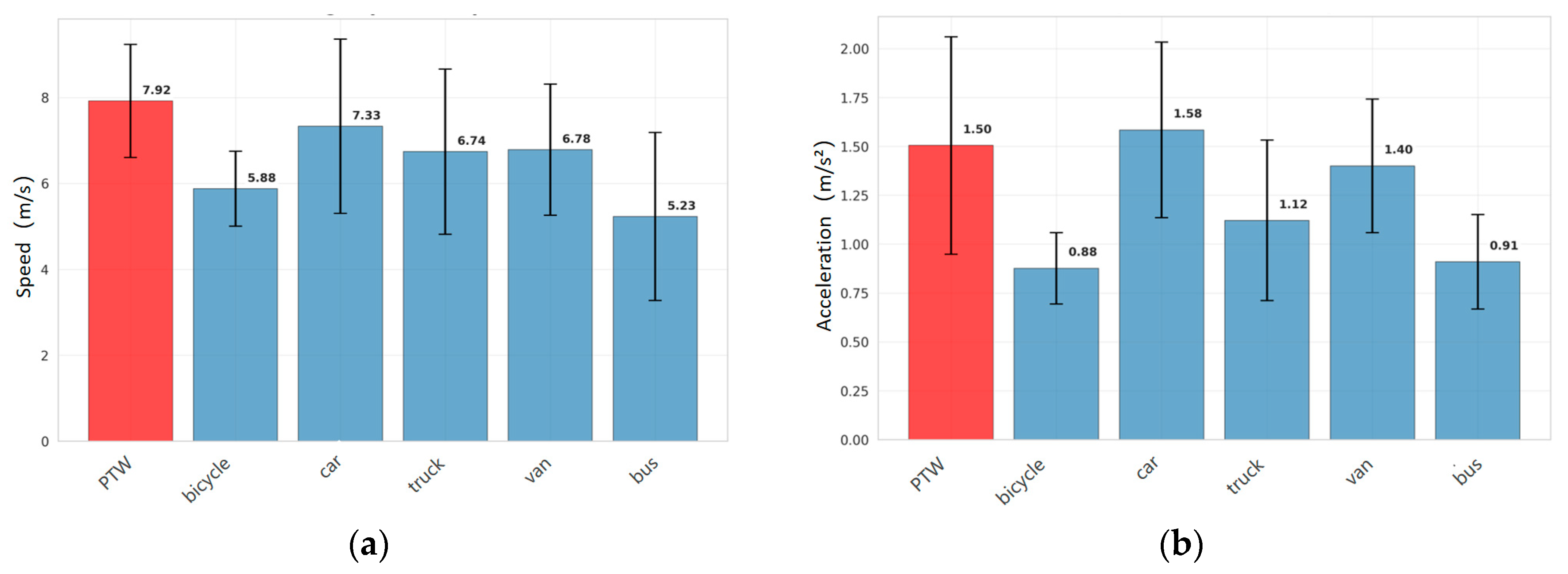
Figure 1. Vehicle performance comparison ((a) average speed comparison; (b) average acceleration comparison; (c) average heading change rate comparison; (d) normalized vehicle performance comparison—radar chart).
Systems 13 01036 g001aSystems 13 01036 g001b
Figure 2. Framework of the PTW trajectory prediction model.
Systems 13 01036 g002
Figure 3. Dynamic interaction graph in mixed traffic scenarios.
Systems 13 01036 g003
Figure 4. The basic overview of the rounD dataset ((a) extracting trajectory and category for each road user through computer vision algorithms; (b) recording traffic at roundabouts by a camera-equipped drone; (c) the specific locations of observation sites (Systems 13 01036 i001 indicates the data collection location of the rounD dataset)).
Systems 13 01036 g004
Figure 5. Variation curves of (a) ADE, (b) FDE, and (c) RMSE during model training.
Systems 13 01036 g005
Figure 6. Training and validation loss curve in the mixed traffic scenario.
Systems 13 01036 g006
Figure 7. Results curves of comparison experiments.
Systems 13 01036 g007
Table 1. Definition of variables used in trajectory prediction modeling.
VariableDefinition
S The set of historical states of i powered two-wheelers (PTWs) in a mixed traffic scenario. S = S 1 , S 2 , S i   .
T The set of time steps for trajectory data. T   =   1 ,   2 ,   3 ,     t h .
t h The total length of historical time steps input to the trajectory prediction model.
i powered two-wheelers (PTWs).
j Surrounding vehicles, mainly including motor vehicles and bicycles.
S i t The historical state of the PTW at time step t input to the model. S i t   =   P i t ,   V i t ,   A i t ,   Heading i t ,   ID i , Type i .
S j t The historical state of surrounding vehicles at time step t input to the model. S j t   =   P j t ,   V j t ,   A j t ,   Heading j t ,   ID j   ,   Type j .
P i t ,   P j t The position coordinates of the PTW and surrounding vehicles at time step t , including the horizontal and vertical coordinates. Among these, P i t = x i t ,   y i t , P j t = x j t ,   y j t .
V i t ,   V j t The velocity information of the PTW and surrounding vehicles at time step t , including the lateral and longitudinal velocities. Among these, V i t = v xi t ,   v yi t , V j t = v xj t ,   v yj t .
A i t ,   A j t The acceleration information of the PTW and surrounding vehicles at time step t , including the lateral and longitudinal accelerations. Among these, A i t = a xi t ,   a yi t , A j t = a xj t ,   a yj t .
Heading i t ,   Heading j t The heading angle of the PTW and surrounding vehicles at time step t .
ID i ,   ID j The identity codes of the PTW and surrounding vehicles, used for trajectory tracking and organization.
Type i ,   Type j The type identifiers of the PTW and surrounding vehicles, used for categorizing and processing trajectory characteristics of different vehicles in the dataset. Among these, Type j = bicycle ,   car ,   truck ,   bus ,   van .
Table 2. Results of comparison experiments.
ModelsEvaluation Metrics
RMSEADE (m)FDE (m)
0.4 s0.8 s1.2 s1.6 s2.0 s
CV0.140.541.182.053.130.782.23
LSTM0.581.151.732.302.531.902.53
Social-GAN0.280.631.311.932.040.911.58
Trajectron++0.230.470.670.791.340.310.89
GAT-LSTM0.310.640.860.931.250.370.76
BATraj0.170.370.570.841.170.590.67
Our Model0.200.310.440.671.080.280.70
Table 3. Results of ablation experiments.
ModulesEvaluation Metrics
Time Attention LayerGAT Interaction LayerFeature FusionPosition CorrectionADE
(m)
FDE
(m)
×0.360.83
×0.530.95
×0.450.86
×0.480.88
××0.651.23
××0.390.98
0.280.70
Disclaimer/Publisher’s Note: The statements, opinions and data contained in all publications are solely those of the individual author(s) and contributor(s) and not of MDPI and/or the editor(s). MDPI and/or the editor(s) disclaim responsibility for any injury to people or property resulting from any ideas, methods, instructions or products referred to in the content.