Assessing the Impact of Socioeconomic and Environmental Indicators on the Consumption Footprint Using Statistical and Neural Network Analyses

Abstract

Understanding the factors that influence the Consumption Footprint (CF) is essential for advancing sustainable development within the European Union. This study investigates the most impactful indicators affecting CF, aligning the analysis with the 17 Sustainable Development Goals (SDGs), which are grouped into five thematic clusters: economic conditions, globalization, health, environmental awareness, and cultural factors. To identify key drivers, the research employs a dual-method approach: Graphical representations and correlation analyses and machine learning via Artificial Neural Networks (ANNs), supported by statistical analysis using non-parametric tests. Data from Romania (2012–2023) were used to evaluate the influence of variables such as Gross Domestic Product (GDP), Price Level Indices (CPI), Unemployment Rate (UNE), and Circular Material Use Rate (CMU) on CF. The results reveal that GDP and CPI are the most influential variables, together accounting for over 64% of the impact on CF, followed by UNE and CMU. The study concludes that economic indicators play a dominant role in shaping consumption-related environmental impact. The proposed framework is replicable and adaptable, offering valuable insights for policymakers and researchers aiming to accelerate progress toward EU sustainability targets.

1. Introduction

This paper aims to identify the most important and influential indicators—namely, independent variables—affecting the evolution of the Consumption Footprint (CF). The study is grounded in the European Union’s targets regarding the Sustainable Development Goals and seeks to determine which indicators, grouped into five general clusters, exert significant influence on the CF. This is considered a key factor in shaping sustainability and accelerating the achievement of the European Union’s objectives. The SDGs, adopted by the United Nations and supported by the European Union, provide a comprehensive framework for sustainable development.

The 17 Sustainable Development Goals (SDGs) are:

Goal 1—No poverty (sdg_01);

Goal 2—Zero hunger (sdg_02);

Goal 3—Good health and well-being (sdg_03);

Goal 4—Quality education (sdg_04);

Goal 5—Gender equality (sdg_05);

Goal 6—Clean water and sanitation (sdg_06);

Goal 7—Affordable and clean energy (sdg_07);

Goal 8—Decent work and economic growth (sdg_08);

Goal 9—Industry, innovation and infrastructure (sdg_09);

Goal 10—Reduced inequalities (sdg_10);

Goal 11—Sustainable cities and communities (sdg_11);

Goal 12—Responsible consumption and production (sdg_12);

Goal 13—Climate action (sdg_13);

Goal 14—Life below water (sdg_14);

Goal 15—Life on land (sdg_15);

Goal 16—Peace, justice and strong institutions (sdg_16);

Goal 17—Partnerships for the goals (sdg_17).

In the context of CF analysis, organizing the 17 SDGs into thematic clusters enhances analytical clarity and policy relevance.

The CF is shaped by a complex interplay of economic, technological, social, environmental, and cultural factors. Understanding these influences is essential for promoting more informed and sustainable consumption behaviors and developing sustainable projects. In alignment with the 17th European SDGs and considering the structural framework of the projects, we categorize the influencing factors as follows:

• Economic Conditions. Economic growth and income levels are key drivers of consumption. As income increases, individuals tend to consume more goods and services, often shifting toward discretionary and luxury items. Moreover, consumption patterns vary across income groups, influencing subjective perceptions of well-being and poverty [1].
• Globalization and Technological Advancements. Globalization has expanded consumer access to international products, fostering diversity in consumption. It also influences cultural identity and self-concept, as individuals navigate multiple cultural affiliations in a globalized marketplace [2]. Digital innovations—such as smartphones, voice assistants, and recommendation systems—have transformed consumer decision-making. These technologies not only facilitate access to products but also shape preferences and choices through intelligent curation [3]. Social media plays a pivotal role in shaping consumer behavior. Peer recommendations, online reviews, and brand conversations significantly affect product valuation and purchasing decisions [4].
• Health. A healthy lifestyle significantly shapes consumer behavior, particularly in the context of food choices and brand preferences. Individuals who prioritize health tend to perceive greater value—social, emotional, and quality-related—in products that align with their wellness goals. This perception enhances their willingness to purchase healthy food brands. However, economic value plays a lesser role in driving these decisions, suggesting that health-conscious consumers are more motivated by quality and emotional connection than by price [5].
• Environmental Awareness. Growing concern for environmental sustainability is influencing consumption patterns, especially among younger generations. Consumers increasingly prefer products with lower environmental impact, although actual behavior often lags behind stated intentions [6].
• Cultural Factors. Cultural norms and values shape consumption habits, including dietary preferences, fashion, and sustainability attitudes. Cultural dimensions such as individualism vs. collectivism influence motivations for sustainable consumption [7].

This paper is significant as it proposes an integrated methodology for identifying the most influential variables affecting the evolution of the CF, a key indicator in sustainability assessment. By organizing the 17th Sustainable Development Goals into five thematic clusters—economic, globalization, health, environment, and culture—the authors provide a clear and applicable analytical framework. The combined use of graphic analysis and artificial neural networks (ANNs) enables a robust analysis of complex relationships between variables, particularly highlighting the role of GDP and the consumer price index. The results can guide public policies and sustainability strategies, contributing to the accelerated achievement of the European Union’s objectives. Moreover, the proposed model is replicable and extensible, offering a solid foundation for future research in responsible consumption and sustainable development.

The remainder of this manuscript is organized as follows: Section 2, Materials and Methods, describes the dataset and evaluates its values, along with the methodologies employed in the research; Section 3, Results, presents the outcomes obtained through these methods and provides an interpretation of the findings; finally, Section 4, Discussion and Conclusions, summarizes the key insights, discusses the study’s limitations, and outlines potential directions for future research.

2. Materials and Methods

To ensure methodological coherence, the study adopts a sequential and complementary dual-method approach that combines statistical analysis with Artificial Neural Networks (ANNs). The rationale for this integration lies in the distinct strengths of each method:

Statistical Analysis (correlation matrices and non-parametric tests) was employed as an initial step to identify significant relationships between variables and the CF. This phase provided objective criteria for variable selection, retaining only indicators with strong correlations (r > 0.7) to ensure analytical rigor.

ANN Modeling was subsequently applied to capture non-linear interactions and assess the relative importance of the selected variables. Unlike traditional statistical methods, ANNs can model complex patterns and provide a hierarchical ranking of influences, offering predictive insights beyond linear assumptions.

This structured approach ensures that the two methods complement each other effectively. Statistical analysis provides a rigorous basis for selecting variables with strong correlations to CF, while ANN modeling captures non-linear relationships and delivers a clear hierarchy of influence. The coherence of this methodology is reinforced by the visual evidence presented in image analysis, which illustrates data distribution, trends, and interaction effects, which quantifies variable importance. The integration of these results is highlighted in the Section 4, where ANN-derived rankings align with correlation-based insights, demonstrating consistency and methodological synergy.

2.1. Data

Based on the types of SDGs and the availability of relevant online data, the 17 SGDs considered in this study were grouped into five distinct categories, as was done in the previous chapter. The limitation in both the number of variables and the amount of data available is mainly due to the short period of recording, which reflects the relatively recent emergence of sustainability monitoring as a widespread objective worldwide. Therefore, the data correspond to a limited time frame. The data used in this study include both dependent and independent variables, as presented below, and were retrieved from the Eurostat website for Romania, covering the period from 2012 to 2023.

Romania provides a complete and consistent dataset covering the years 2012 to 2023, which supports the effective use of both statistical and machine learning methods. As a member of the European Union, Romania follows common sustainability targets and policy frameworks, offering relevant insights into areas such as the circular economy, economic growth, and environmental awareness within the EU context. Its status as a transitional economy with shifting consumption patterns makes it a valuable case for examining the relationship between socioeconomic indicators and environmental impact. The methodological framework developed in this study, piloted on Romania, is designed to be replicable and scalable to other EU countries in future research. Furthermore, based on the premise that the present analysis serves as a foundation for future, more in-depth research, the selection of data reflecting Romania’s situation is justified by the authors’ ability to assess the accuracy of the research outcomes, given their comprehensive understanding of the real context from the perspective of the country’s citizens.

Following the categories defined above and combining them with variables that were already recorded and available online, the following variables were identified and assigned to each category. Although some variables span a period beyond 2011–2023, only this interval contains complete data for all variables. Following the categories defined above and combining them with variables that were already recorded and available online, the following variables were identified and assigned to each category.

• Economic conditions variables

Gross Domestic Product (GDP) per capita in Purchasing Power Standards is measured relative to the EU average, set at 100. Values above 100 indicate a higher GDP per capita than the EU average; values below 100 indicate a lower level. While commonly used to compare economic well-being across countries, GDP includes elements that may not fully reflect household living standards. Purchasing Power Standards (PPS), a notional currency used by Eurostat, adjusts for price level differences between countries, enabling meaningful comparisons [8].

Price Level Indices (CPI) reflect household final consumption expenditure, adjusted using purchasing power parities (PPPs), and are expressed as an index with the EU-27 average set at 100. A value above 100 indicates relatively higher prices compared to the EU average, while a value below 100 suggests lower prices. The data refer to the EU-27 as defined in 2020, excluding the United Kingdom [9].

Companies are assessed on how they engage with their employees, including job satisfaction, training, and development opportunities. Creating inclusive spaces where everyone, regardless of background, can thrive is fundamental. This involves ensuring equitable access to resources and opportunities [10]. The Unemployment Rate (UNE) represents the share of unemployed individuals within the total labor force, which includes both employed and unemployed persons. Unemployed individuals are defined as those aged 15 to 74 who were without work during the reference week, available to start work within two weeks, and actively seeking employment within the preceding four weeks or had secured a job to begin within three months. This indicator is based on data from the EU Labour Force Survey [11].

• Globalization variable

KOF Globalization Index (KOF) [12], developed by the KOF Swiss Economic Institute, measures the extent of globalisation in countries across three dimensions: economic, social, and political. It distinguishes between actual flows (de facto) and enabling policies (de jure) and uses over 40 variables to assess integration. Scores range from 1 to 100, with higher values indicating greater globalization. The index is updated annually and is widely used for cross-country comparisons and academic research.

• Health variable

A healthy population is more capable of contributing to sustainable development. Access to healthcare and promoting healthy lifestyles are vital for a strong, sustainable society. Healthy life years at birth by sex (HLY)—measures the number of years that a person at birth is still expected to live in a healthy condition. It combines information on mortality and morbidity. A healthy condition is defined by the absence of limitations in functioning/disability. The indicator is also called disability-free life expectancy [13].

• Environmental awareness variables

Active participation in community initiatives fosters a sense of belonging and responsibility. Community gardens, for example, not only provide fresh produce but also strengthen social bonds and promote environmental stewardship. Share of renewable energy in gross final energy consumption (SRE). The indicator measures the share of renewable energy consumption in gross final energy consumption according to the Renewable Energy Directive. The gross final energy consumption is the energy used by end-consumers (final energy consumption) plus grid losses and self-consumption of power plants [14]. The Circular Material Use Rate (CMU) indicates the proportion of recovered materials reintroduced into the economy relative to total material use. It is calculated as the ratio of the circular use of materials to the overall material use. Circular use is approximated by the amount of waste recycled domestically, adjusted for imports and exports of waste for recovery [15]. A higher CMU reflects greater substitution of secondary materials for primary raw materials, contributing to reduced environmental impact [16].

CMU ensuring fairness and equal opportunities for all members of society helps build a more resilient and cohesive community. This includes addressing social inequalities and promoting inclusivity. Persons employed in circular economy sectors (ECE) indicator measures the number of persons employed in three key circular economy sectors: recycling, repair and reuse, and rental and leasing. Employment is reported both as an absolute number and as a percentage of total employment. It includes all individuals working within the reporting unit (e.g., firm), such as owners, partners, and unpaid family workers, as well as those working externally but paid by the unit. It excludes personnel supplied by other enterprises and those performing external maintenance or serving in compulsory military service [17].

• Target variable

The Consumption Footprint indicator assesses the environmental impact of EU consumption using life cycle data from approximately 165 representative products across five sectors: food, mobility, housing, household goods, and appliances. It combines product-specific consumption intensity with emissions and resource use, applying the Environmental Footprint method to quantify 16 impact categories. These are aggregated into a single score that reflects how often planetary boundaries are exceeded [18].

This clustering approach aligns with previous studies that emphasize multidimensional influences on sustainability [6,7].

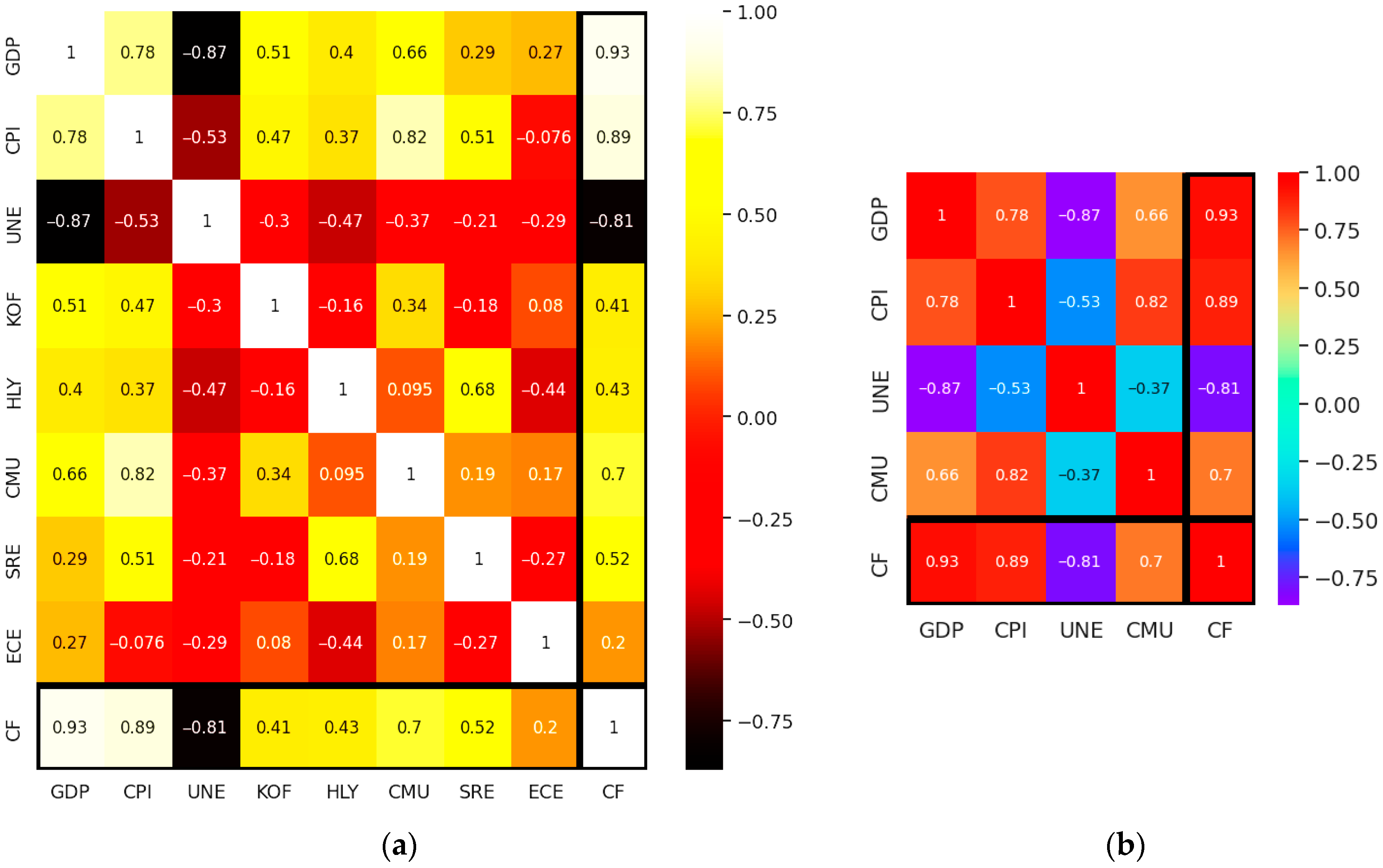
To identify the most influential indicators affecting the CF, a preliminary correlation analysis was conducted across all available socioeconomic and environmental variables, involving constructing a correspondence matrix that quantifies the strength of correlations in numerical form. The correlations are considered stronger as their values increase, as illustrated in Figure 1. Only those variables with a correlation coefficient greater than 0.7 with CF were retained for detailed analysis, ensuring a statistically significant and meaningful relationship with the target variable. Based on this criterion, four variables were selected: Gross Domestic Product (GDP), Price Level Indices (CPI), Unemployment Rate (UNE), and Circular Material Use Rate (CMU). Figure 1a displays all variables, while Figure 1b includes only those variables with a correlation coefficient of 0.7 or higher with respect to CF.

For easier presentation and to simplify tracking the research, from now on the use of all independent variables in methods and algorithms will be denoted as all_var, while the use of only the four independent variables considered more influential will be denoted as 4_var. From this point onward, all analyses concerning the variables will be conducted for both the all_var and 4_var datasets, thereby enhancing analytical clarity and methodological rigor.

To assess the internal consistency of the data, their heterogeneity, potential common variations, or simply to observe the correlations among variables, several tests were implemented. The lack of strong correlations between certain variables prompted the application of a wide range of tests in an effort to identify possible relationships. The tests applied are as follows:

• Cronbach’s Alpha—used to assess internal consistency.
• Shapiro–Wilk Test—tested for normality.
• Bartlett’s Test—assessed homogeneity of variances.
• Kruskal–Wallis and Mann–Whitney U Tests—used to detect differences between groups.

The detailed methodological explanations, which include formulas, assumptions, and interpretation guidelines, are presented in Appendix A.

The reliability analysis of the scale reveals significant issues, as indicated by the negative Cronbach’s alpha values. For the full scale of values (all_var), the alpha is −1.785 with a confidence interval ranging from −4.969 to 0.061. This suggests severe inconsistency, potentially due to small amount of data. The confidence interval includes zero, further emphasizing the unreliability of the scale. Similarly, for the subset (4_var), the alpha is −2.448 with a confidence interval entirely below zero [−6.935, −0.132]. The analysis shows that is a very low or zero variance (items have little, the covariance matrix becomes unstable) or there are too few items or small sample size (with very few items or a small number of observations, alpha can behave erratically). These results strongly suggest that the data requires further analysis.

For the full sample (all_var), the test statistic is 0.856 with a p-value of 7.84 × 10⁻⁹, indicating a significant deviation from a normal distribution. Similarly, for the subset of four groups (4_var), the test statistic is 0.878 and the p-value is 2.26 × 10⁻⁵, again rejecting the null hypothesis of normality. These consistently low p-values confirm that the data does not follow a normal distribution, which has important implications for the choice of statistical methods. Non-parametric approaches may be more appropriate given these results.

The Bartlett’s test results indicate significant heterogeneity of variances across the groups. For the full dataset (all_var), the test statistic is 177.27 with an extremely low p-value of 3.85 × 10⁻³⁴, strongly rejecting the null hypothesis of equal variances. Similarly, for the subset of four groups (4_var), the test statistic is 64.68 with a p-value of 3.00 × 10⁻¹³, again confirming significant differences in group variances. These findings provide strong evidence of heteroscedasticity and suggest that the assumption of homogeneity of variances is debased. Given the small sample size and the lack of normality, parametric tests such as ANOVA or t-tests may not be appropriate. Instead, non-parametric alternatives like the Kruskal-Wallis test or the Mann-Whitney U test should be considered for more reliable statistical inference.

The results of the analysis conducted using the two selected tests are summarized in

Table 1. Results of Kruskal–Wallis test, the Mann–Whitney U test.

Indicator	Test Statistic	p-Value	Conclusion	Test
GDP	17.295	0.00003200	Significantly different	Kruskal-Wallis test
CPI	17.288	0.00003213	Significantly different
UNE	17.318	0.00003162	Significantly different
KOF	17.280	0.00003226	Significantly different
HLY	17.303	0.00003188	Significantly different
CMU	0.857	0.35466787	Not significantly different
SRE	10.673	0.00108692	Significantly different
ECE	10.285	0.00134088	Significantly different
GDP	144.00	0.00003630	Significantly different	Mann-Whitney U test
CPI	144.00	0.00003644	Significantly different
UNE	144.00	0.00003588	Significantly different
KOF	144.00	0.00003658	Significantly different
HLY	144.00	0.00003616	Significantly different
CMU	88.00	0.36990627	Not significantly different
SRE	128.50	0.00120332	Significantly different
ECE	16.50	0.00148197	Significantly different

Source: Authors’ calculation.

.

The results of both the Kruskal-Wallis and Mann-Whitney U tests indicate statistically significant differences across groups for most indicators, including GDP, CPI, UNE, KOF, HLY, SRE, and ECE, as evidenced by extremely low p-values.

These findings suggest that these variables vary meaningfully between the compared groups. However, the CMU indicator does not show significant differences in either test, indicating a lack of variation across groups for this variable. Overall, the consistency between the two non-parametric tests reinforces the robustness of the observed differences and supports the use of non-parametric methods given the data characteristics.

Based on the results of the applied tests and the observation of significant nonlinearity in the evolution of the variables, it was deemed necessary to apply specific methods, which are presented in the following subsection.

2.2. Methods

The present research employs two distinct methodological approaches. The first method involves applying graphical representation techniques to observe the evolution of the dependent variable (CF) in relation to the four selected independent variables (GDP, CPI, UNE, CMU). The second method employs Artificial Neural Networks (ANN), a branch of Artificial Intelligence, to determine the hierarchy of the observed influences. To illustrate the evolution of each indicator and to concatenate these trends, several Python (version 3.11) modules and functions were utilized. Among the key tools applied within the first method are:

• sns.lineplot—Plots a line plot with possibility of several semantic groupings [19].
• sns.jointplot—Draws a plot of two variables with bivariate and univariate graphs [20].
• sns.regplot—The regplot generates a single scatter plot of data with a linear regression through the data points complete with a 95% confidence interval [21].
• corrmat—Creates a correlation Matrix. Correlation matrix is a table that shows how different variables are related to each other [22].
• curve_fit—Uses non-linear least squares to fit a function [23]. Due to the small number of values and their distribution, a fourth-degree function was used.
• ax.plot_surface—Creates a surface plot [24].
• np.polyfit—is a function that performs least squares polynomial fitting. It fits a polynomial of a specified degree to a set of data points, minimizing the squared error between the polynomial and the data [25].

For the second method, the ANN used is a feedforward type implemented with MLPRegressor (Multi-Layer Perceptron Regressor), both well-known and widely used variants. MLPRegressor is a supervised learning algorithm in the scikit-learn library used for regression tasks [26]. It models complex relationships between input features and a continuous target variable by training a feedforward neural network. The model optimizes the squared error using either the Limited-memory Broyden–Fletcher–Goldfarb–Shanno algorithm or stochastic gradient descent (SGD), and supports various activation functions such as ReLU, tanh, and logistic. It is particularly useful for capturing non-linear patterns in data and can be customized with multiple hidden layers and neurons.

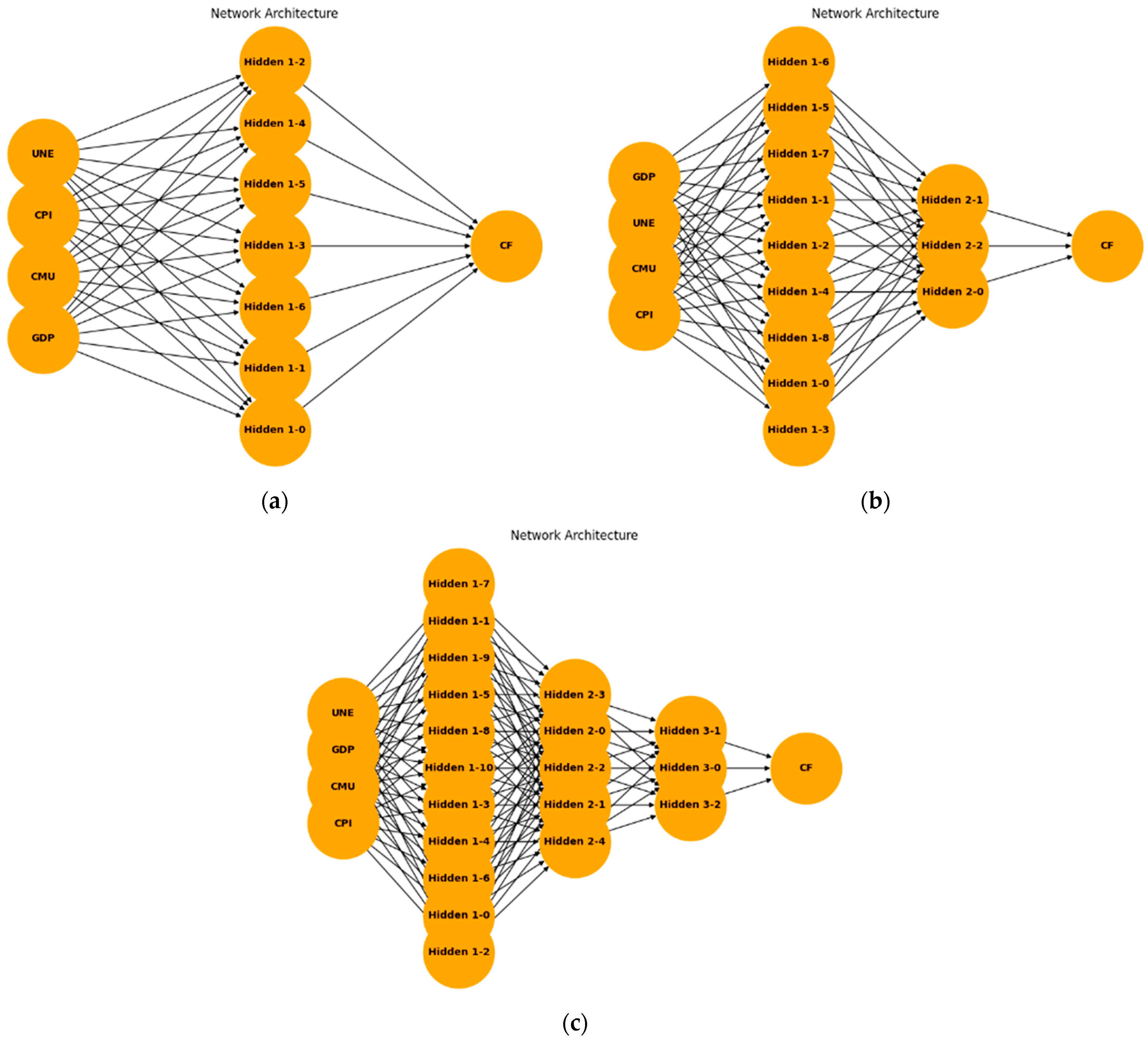
To determine the optimal internal structure of the ANN (i.e., the number of hidden layers and hidden neurons), several configurations were tested and evaluated, examples of these structures are shown in Figure 2. The selected variant is presented in Section 3—Results. The general characteristics used across all these internal structures are summarized in

Table 2. General training’s settings for all ANN’s architecture.

Settings	Values/Types
Learning rate type	adaptive
Learning rate value	0.01
Batch size	2
Activation function	relu/tanh
Solver	adam/sgd
No. of iteration without error change	500

Source: Authors’ calculation.

.

ReLU (Rectified Linear Unit Activation Function) outputs the input if positive, otherwise zero [27]. It’s fast and widely used in deep learning. Tanh (Hyperbolic Tangent Activation Function) maps input values to the range (−1, 1). It’s smoother than ReLU and often used in recurrent neural networks [28]. The adam solver (short for Adaptive Moment Estimation) is a popular optimization algorithm used in training machine learning models, especially deep neural networks [29]. SGD (Stochastic Gradient Descent Optimizer) is a basic optimization algorithm that updates model parameters using gradients from random batches. It can be enhanced with momentum and learning rate decay [30].

The dataset was divided into training and testing subsets using the parameter test_size = 0.05, which resulted in a testing set containing only a single value. This configuration was necessitated by the limited number of training sets (12) and the authors’ intention to prioritize the training process. Consequently, it was considered that calculating the R² score for the testing phase would offer limited relevance for evaluating the performance of the artificial neural network (ANN). Also, due to the limited sample size k-fold cross-validation was not applied.

The final structure selected for further application will be detailed in the following chapter and is based on the evaluation of both training error and training score.

3. Results

The results of the applied methods are presented in the following section, in alignment with the methodological sequence—starting with graphical representations and concluding with the implementation of artificial neural networks (ANNs).

3.1. Applying Graphical Representation

The results of applying the sns.jointplot function, highlighting areas of value concentration, are presented in Figure 3.

The graphical analysis revealed distinct patterns in how each variable relates to the CF (the higher the density, the darker the color (blue)):

• GDP showed a moderately scattered distribution with a central concentration, indicating a stable and interpretable influence on CF.
• CPI exhibited tighter clustering and stronger density contours, suggesting a more pronounced but potentially non-linear relationship.
• UNE presented a broader spread with localized density, implying variable influence across different ranges.
• CMU displayed the weakest correlation, with dispersed data and low-density contours, indicating minimal direct impact on CF.

The table below (

Table 3. graphical analysis including data point distribution, density contours, and histograms.

Variable	Distribution of Data Points	Density Contours	Histograms
GDP	Moderately scattered with central concentration	Medium-density area around center	Fairly even distribution
CPI	Tightly clustered	High-density zone	Concentrated distribution
UNE	Wider spread with dense region	Complex density variation	Broad distribution
CMU	Widely dispersed	Uniform spread, low density	Broadly distributed

Source: Authors’ calculation.

) summarizes the distribution characteristics of four key variables—GDP, CPI, UNE, and CMU—in relation to the CF, based on graphical analysis including data point distribution, density contours, and histograms.

Among the variables analyzed, GDP and UNE show the strongest influence on CF, supported by clear density patterns and concentrated distributions. CPI has a moderate and stable impact, while CMU appears to have the least effect, with no evident correlation. These insights indicate that CF is most sensitive to changes in GDP and UNE, making them potentially key variables in predictive modeling or economic analysis.

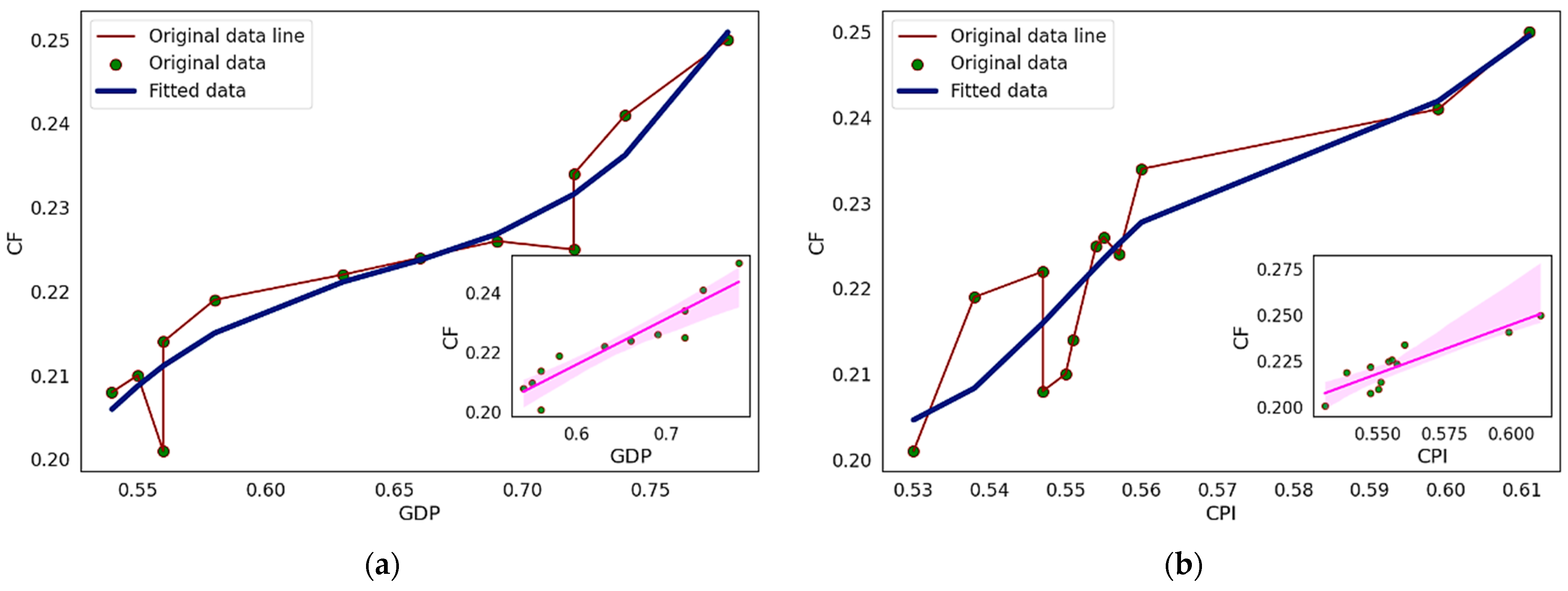
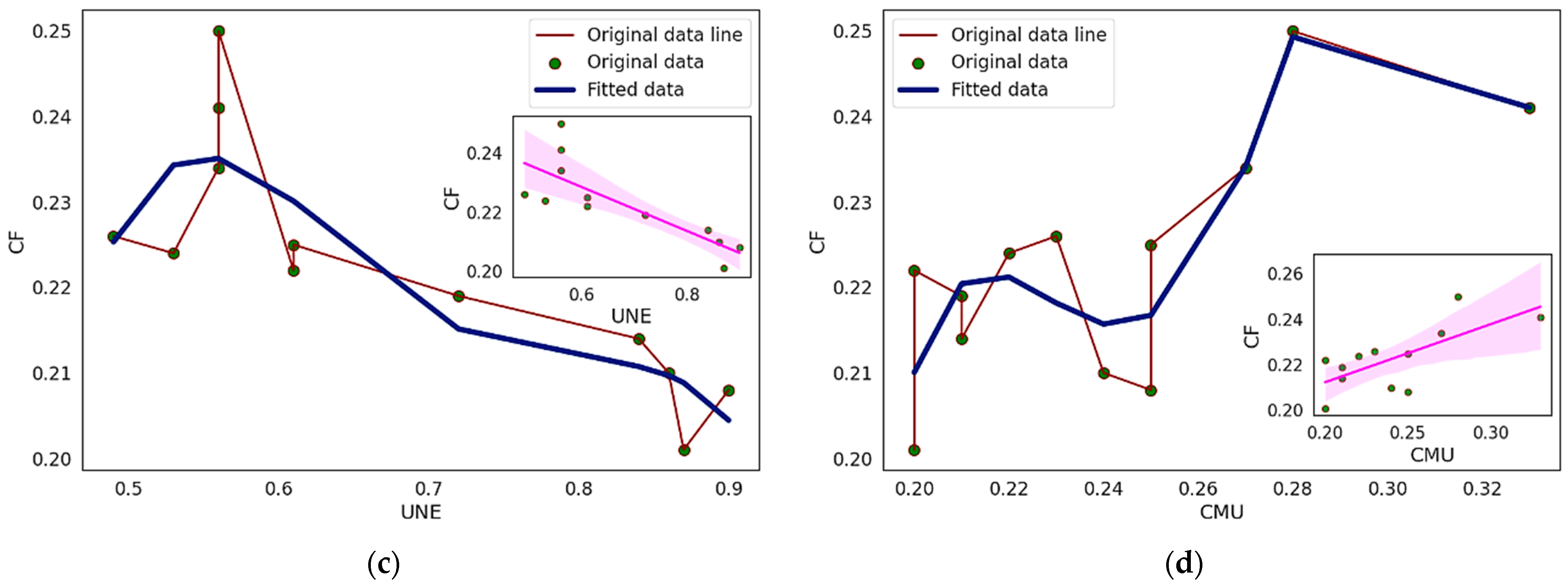
Figure 4 displays four types of graphical representations: the scatter plot of the original data (in green), a red line indicating the evolution of original data, the fitted data shown in blue, and the linear regression line in pink. All these graphs support the analysis of the evolution of the independent variables in relation to CF, as well as their slope and curvature.

The original data from plot Figure 4a, represented by green dots, shows moderate dispersion across the plot. The red line, which traces the original data trend, follows a smooth and consistent path. The fitted data, shown in blue, aligns closely with the original trend, particularly in the zoomed-in inset where the fit is most evident.

Table 4. Graphical analysis including original data, data trends and fitted data.

Variable	Original Data	Data Trend	Fitted Data
GDP	Relatively stable and well-modeled	Consistent trend, moderate and predictable influence on CF	Good approximation of overall trend
CPI	More scattered, indicating greater variability	General direction captured, but variability implies complex relationship	Visible deviations in certain areas
UNE	Noticeable spread and irregularity	Fluctuations and curvature, non-linear and variable relationship	Mismatches in specific regions, struggles to account for irregularities
CMU	Widely dispersed, with no clear pattern	Weakest alignment, minimal direct influence on CF	Fails to capture coherent trend

Source: Authors’ calculation.

summarizes the distribution characteristics of four key variables—GDP, CPI, UNE, and CMU—in relation to the CF, based on graphical analysis including original data, data trends and fitted data.

Among the variables analyzed, GDP shows the most consistent and well-fitted relationship with CF, making it a reliable predictor. CPI and UNE exhibit more complex and variable influences, with CPI being moderately predictable and UNE displaying non-linear behavior. CMU has the least impact, characterized by poor model fit and high data dispersion. These findings reinforce the idea that GDP is a stable driver of CF, while CPI and UNE require more sophisticated modeling approaches to accurately capture their effects. CMU may not be a significant factor in explaining variations in CF.

Next, 3D surface plots were implemented, which illustrate how a dependent variable (e.g., CF) changes in response to two independent variables (e.g., GDP and CPI). These plots help visualize:

• The strength and direction of influence each variable has;
• Nonlinear relationships and interaction effects;
• Steep slopes indicate a strong impact but are harder to simulate if the relationship is nonlinear, while flat areas suggest a weaker influence but are easier to model.

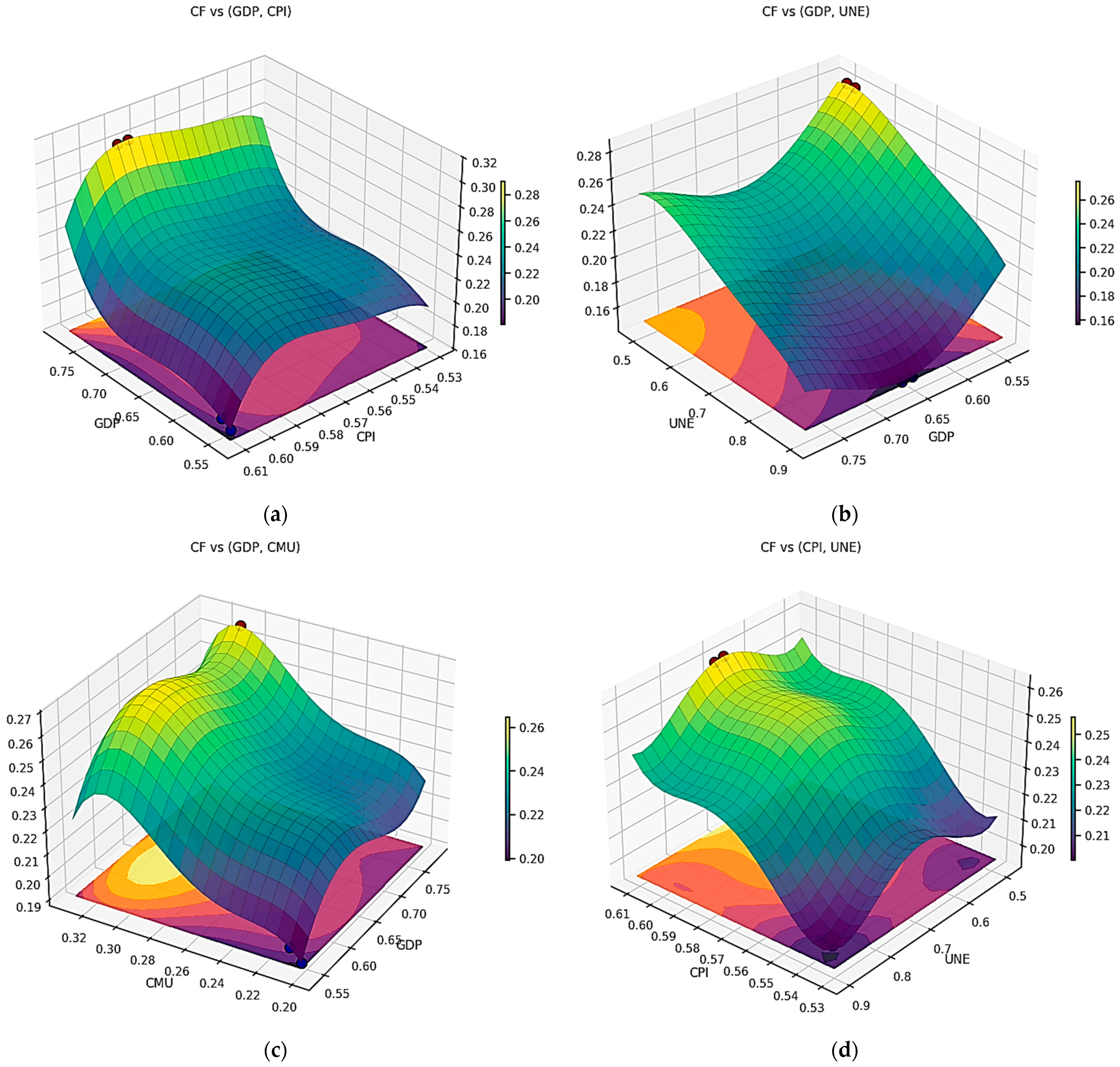
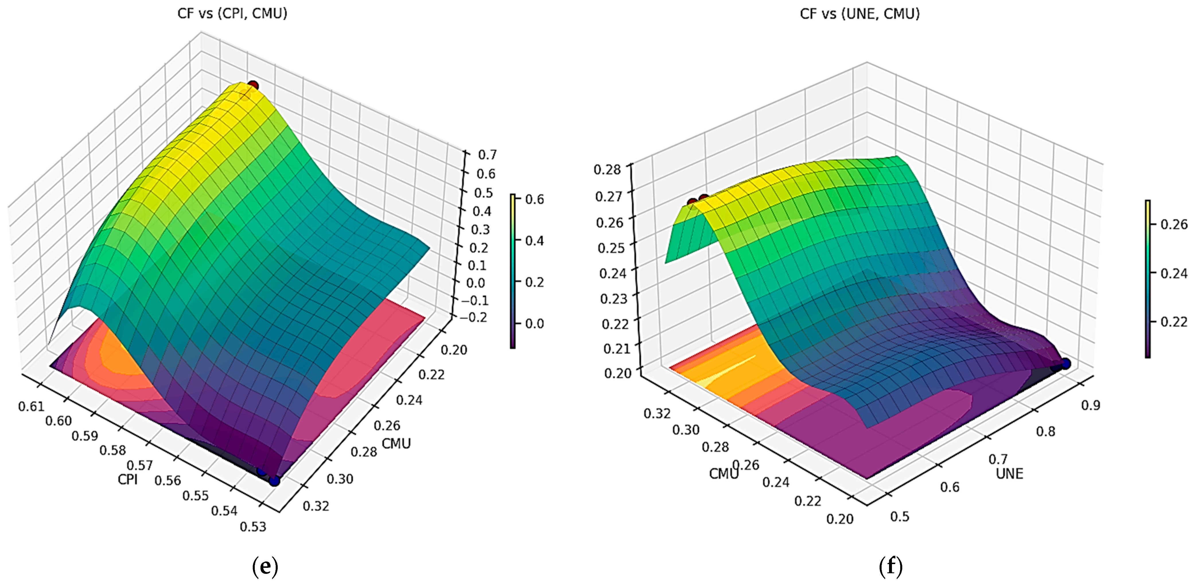
In Figure 5, more abrupt slope (or steeper surface) indicate stronger influence of a variable on CF and more complex surfaces suggest interaction effects and non-linear relationships. Also, variables that repeatedly show strong effects (same effects) across multiple plots are likely more influential.

In Figure 5a GDP is easier to follow, with fewer curvature changes, slightly steeper than CPI. CPI is more dynamic, with greater slope and curvature variation. Interpretation: While CPI shows stronger influence, GDP’s smoother behavior makes it more practical for modeling. Conclusion: Both variables are influential, but GDP is more stable and easier to interpret.

Next Figure 4b, shows that GDP is steeper and more consistent than UNE, and UNE has a Moderate influence, relatively stable but less steep. Interpretation: GDP dominates in terms of impact and usability; UNE contributes to smoother transitions but with limited influence. Conclusion: GDP is the key variable; UNE is secondary and less impactful.

In Figure 5c GDP is less steep than CMU, but with fewer curvature changes, while CMU is steeper and more nonlinear, harder to interpret. Interpretation: CMU’s volatility reduces its usefulness; GDP remains the more reliable variable. Conclusion: GDP is preferable for modeling CF; CMU is too erratic.

A revealed in Figure 5d CPI is much steeper than UNE, with more curvature, as UNE is balanced and less volatile. Interpretation: CPI has a stronger but more fluctuating impact; UNE offers smoother transitions. Conclusion: CPI is dominant but harder to model; UNE is stable but less influential.

CPI has a strong influence, in Figure 5e, with significant slope and curvature, and CMU is steep but highly nonlinear, difficult to use. Interpretation: CPI is more usable despite its fluctuations; CMU’s instability limits its value. Conclusion: CPI is the most effective variable; CMU is negligible.

In the last Figure 5f UNE is less steep and more stable, while CMU is steeper but with excessive curvature. Interpretation: Neither variable shows strong or usable influence; both are weak contributors. Conclusion: This combination is the least informative for modeling CF.

Overall Conclusion:

• GDP: Offers a more stable and consistent contribution to CF, making it easier to interpret and model, even if slightly less impactful than CPI;
• CPI: Has the strongest influence on CF but is highly dynamic, with steep slopes and curvature changes. Useful but harder to model;
• UNE: Provides a moderate and smooth influence, but lacks strength in driving CF variation;
• CMU: Is steep and nonlinear, making it the least useful variable for modeling CF.

3.2. Applying ANN

The first step in applying ANNs involves determining the optimal internal structure and network characteristics to achieve the lowest possible training error.

Table 5. MLP Train performance. The results of the training and testing processes are presented for mae (Mean Absolute Error) and mse (Mean Squared Error), for both types of neural networks: ReLU with Adam optimizer and tanh with sgd optimizer.

	relu_adam					tahn_sgd
Structure	train_mae	train_mse	test_mae	test_mse	Batch	train_mae	train_mse	test_mae	test_mse
3	0.091641	0.009365	0.351572	0.123603	2	0.020429	0.000659	0.196605	0.038654
5	0.018154	0.000508	0.191466	0.036659		0.009116	0.000188	0.315603	0.099605
7	0.004565	0.000030	0.241717	0.058427		0.019347	0.000517	0.299656	0.089794
9	0.005663	0.000052	0.312752	0.097814		0.018757	0.000503	0.272436	0.074221
11	0.004816	0.000038	0.283183	0.080193		0.016226	0.000396	0.433591	0.188001
(7, 3)	0.004991	0.000079	0.289356	0.083727		0.012665	0.000259	0.157976	0.024956
(7, 5)	0.004202	0.000029	0.401818	0.161458		0.014445	0.000316	0.176232	0.031058
(9, 3)	0.020282	0.001557	0.256201	0.065639		0.012844	0.000232	0.176966	0.031317
(9, 5)	0.001617	0.000004	0.311531	0.097052		0.012850	0.000277	0.376260	0.141571
(9, 7)	0.006979	0.000064	0.321017	0.103052		0.014675	0.000314	0.265022	0.070237
(11, 3)	0.004132	0.000025	0.307319	0.094445		0.016546	0.000377	0.184856	0.034172
(11, 5)	0.009022	0.000106	0.289825	0.083999		0.013224	0.000270	0.192924	0.037220
(11, 7)	0.002865	0.000010	0.257168	0.066135		0.009559	0.000154	0.311000	0.096721
(11, 9)	0.002880	0.000012	0.305964	0.093614		0.011044	0.000247	0.126320	0.015957
(11, 7, 3)	0.012299	0.000347	0.290862	0.084601		0.009880	0.000164	0.300916	0.090550
3	0.010529	0.000210	0.071842	0.005161	10	0.021888	0.000691	0.136415	0.018609
5	0.011701	0.000194	0.036446	0.001328		0.019032	0.000572	0.301698	0.091022
7	0.012604	0.000264	0.053137	0.002824		0.019837	0.000561	0.313816	0.098480
9	0.004126	0.000032	0.082135	0.006746		0.022618	0.000671	0.411375	0.169230
11	0.002319	0.000007	0.080373	0.006460		0.017603	0.000397	0.022822	0.000521
(7, 3)	0.003835	0.000021	0.028261	0.000799		0.013405	0.000270	0.421143	0.177361
(7, 5)	0.010040	0.000145	0.010812	0.000117		0.020497	0.000739	0.577472	0.333474
(9, 3)	0.003237	0.000014	0.079359	0.006298		0.020628	0.000643	0.279601	0.078177
(9, 5)	0.001699	0.000004	0.023428	0.000549		0.015882	0.000406	0.437467	0.191378
(9, 7)	0.004002	0.000023	0.090012	0.008102		0.022570	0.000605	0.041390	0.001713
(11, 3)	0.024801	0.000861	0.126712	0.016056		0.026733	0.000923	0.160771	0.025847
(11, 5)	0.001638	0.000004	0.028097	0.000789		0.019877	0.000527	0.183269	0.033587
(11, 7)	0.003739	0.000019	0.060645	0.003678		0.021401	0.000649	0.375592	0.141070
(11, 9)	0.011678	0.000165	0.066278	0.004393		0.013277	0.000282	0.154537	0.023882
(11, 7, 3)	0.002066	0.000007	0.021839	0.000477		0.016882	0.000409	0.175754	0.030890
3	0.149170	0.033702	0.546881	0.299079	20	0.079502	0.008306	0.029899	0.000894
5	0.007263	0.000094	0.506114	0.256152		0.053927	0.004382	0.090439	0.008179
7	0.031153	0.001736	0.167186	0.027951		0.045266	0.002845	0.104119	0.010841
9	0.007137	0.000101	0.347443	0.120717		0.044810	0.002884	0.108131	0.011692
11	0.010858	0.000235	0.833500	0.694723		0.047858	0.003178	0.104588	0.010939
(7, 3)	0.002533	0.000011	0.405441	0.164383		0.056138	0.004416	0.045948	0.002111
(7, 5)	0.002832	0.000015	0.258917	0.067038		0.045785	0.004041	0.122020	0.014889
(9, 3)	0.005382	0.000067	0.288988	0.083514		0.062158	0.005892	0.073902	0.005462
(9, 5)	0.013190	0.000305	0.468289	0.219295		0.028208	0.001175	0.083037	0.006895
(9, 7)	0.005863	0.000092	0.295006	0.087029		0.042655	0.002803	0.086398	0.007465
(11, 3)	0.004709	0.000071	0.134288	0.018033		0.035892	0.001914	0.076595	0.005867
(11, 5)	0.005770	0.000075	0.557366	0.310657		0.034558	0.001597	0.148793	0.022139
(11, 7)	0.001781	0.000008	0.295189	0.087137		0.048404	0.002944	0.122672	0.015048
(11, 9)	0.004437	0.000063	0.179088	0.032073		0.042594	0.002767	0.114558	0.013123
(11, 7, 3)	0.004768	0.000058	0.080422	0.006468		0.046416	0.003028	0.076354	0.005830
Min	0.001617	0.000004	0.010812	0.000117		0.009116	0.000154	0.022822	0.000521
		Min relu_adam vs. than_sgd				0.001617	0.000004	0.010812	0.000117

Source: Authors’ calculation.

presents a selection of the evaluated network structures, which are compared based on four error metrics: training error, expressed as both Mean Absolute Error (mae) and Mean Squared Error (mse), and testing error, also expressed in the same two forms. Another differentiating factor is the batch value that refers to a subset of the dataset used in one iteration of model optimization [31]. The batch size influences training efficiency and model performance by controlling how often weights are updated during learning. The batch sizes selected by the researchers were 2, 10, and 20.

To facilitate a clearer visualization of the training results and corresponding training errors, Figure 6 has been developed.

Since the comparison of training errors yielded different results for training and testing phases—resulting in distinct structures and varying batch values—a new evaluation metric was introduced in the form of the Train R² Score. MLP (Multilayer Perceptron) Train R² Score refers to the coefficient of determination calculated during the training phase of an MLP regression model [32]. It measures how well the model’s predictions fit the actual training data. A score of 1.0 indicates perfect prediction, while 0 means the model does not explain any of the variability in the target variable. The results of this evaluation are presented in

Table 6. MLP Train R² Score for all ANNs’ structures.

	Batch Number
Structure	2	10	20	2	10	20
	than_sgd			relu_adam
3	0.997963	0.988678	0.869912	0.996055	0.937743	0.843557
5	0.999908	0.994041	0.948313	0.998831	0.997494	0.990658
7	0.998554	0.999736	0.997606	0.999792	0.996281	0.996847
9	0.997189	0.997706	0.972909	0.995539	0.996023	0.995237
11	0.999197	0.994034	0.995193	0.997628	0.990635	0.999966
(7, 3)	0.997592	−0.022910	0.993218	0.987146	0.995476	0.999929
(7, 5)	0.996834	0.999312	0.990236	0.985755	0.987440	0.956785
(9, 3)	0.948170	0.993604	0.898490	0.998116	0.996867	0.972333
(9, 5)	0.986947	0.993855	0.997416	0.999066	0.998511	0.996316
(9, 7)	0.995878	0.987195	0.998150	0.999691	0.999624	0.999605
(11, 3)	0.997565	0.996152	0.999694	0.972995	0.990862	−0.000180
(11, 5)	0.996094	0.999899	0.995200	0.996439	−0.000360	0.994340
(11, 7)	0.996328	0.999052	0.984302	0.999809	0.999592	0.980697
(11, 9)	0.997754	0.998901	0.999153	0.993065	0.999931	0.993057
(11, 7, 3)	0.999383	0.999175	−0.004469	0.999713	0.958768	0.999812
Max Train R2 Score	0.999908	0.999899	0.999694	0.999809	0.999931	0.999966

Source: Authors’ calculation.

.

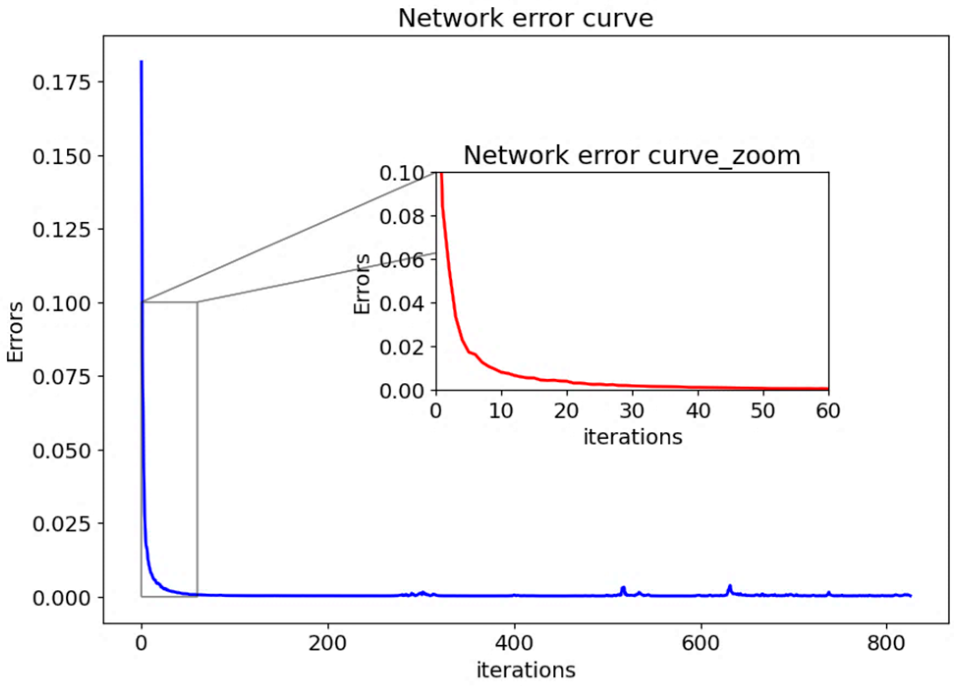
The comparison in Table 6 shows that the score of the (9, 5) AAN’s structure is superior to that of the (7, 5) structure. It can also be observed that the structure with the highest training score (R²) is the one with only 11 neurons in a single hidden layer. Therefore, from this point onward in the present study, the (9, 5) structure will be used. To support this choice, the following figures present elements related to the evaluation of the training process. Figure 7 illustrates the decrease in training error over the course of the iterations.

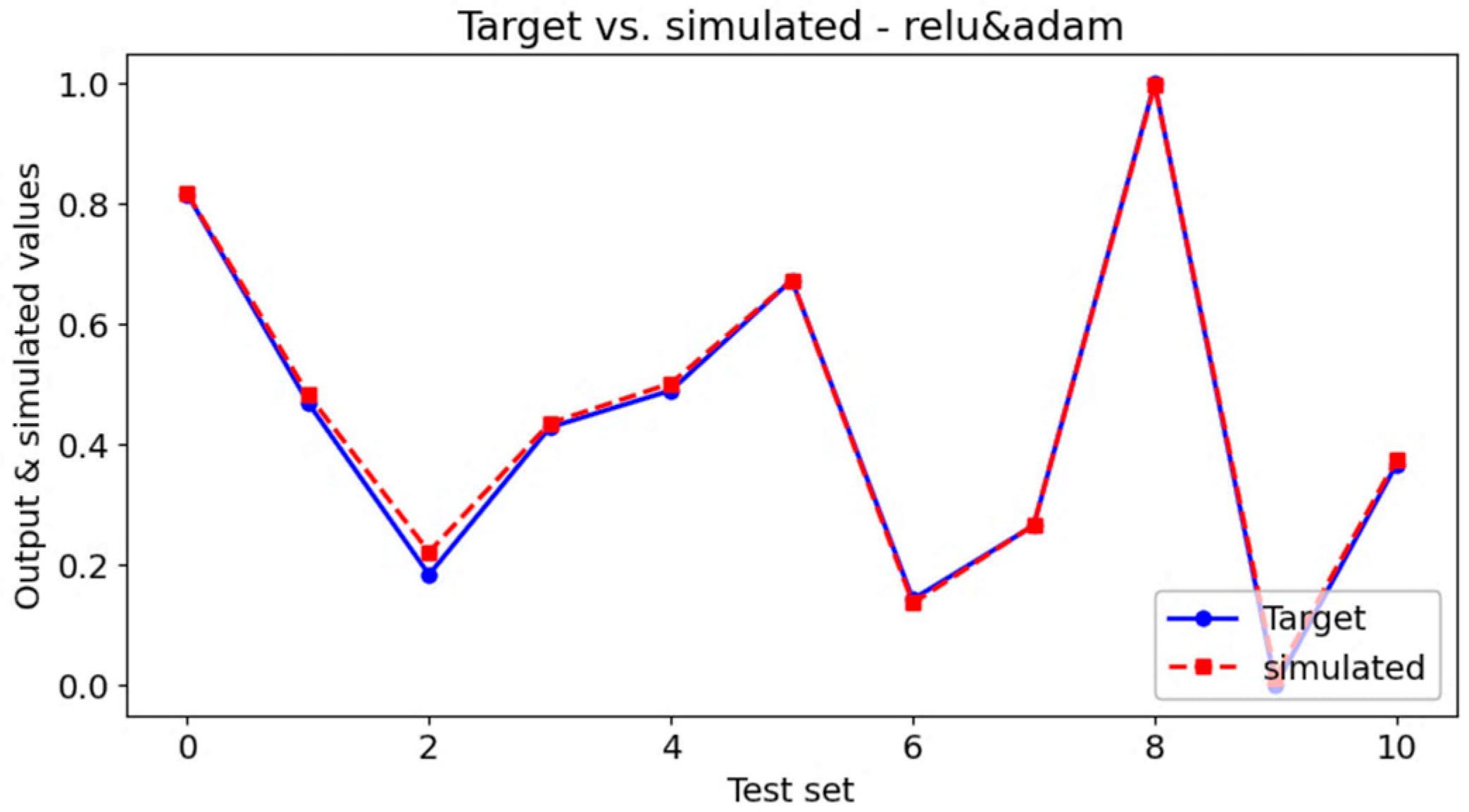
In Figure 8, a comparison can be seen between the target values—these are the actual values used for training the network, shown in blue—and the values simulated by the network after training, represented by a dashed red line.

As can be seen, the two lines (or points) are nearly overlapping, which indicates that the simulation performed by the ANN produced values very close to the target ones. This can be interpreted as a highly accurate training, further supported by the high training score (MLP Train R² Score).

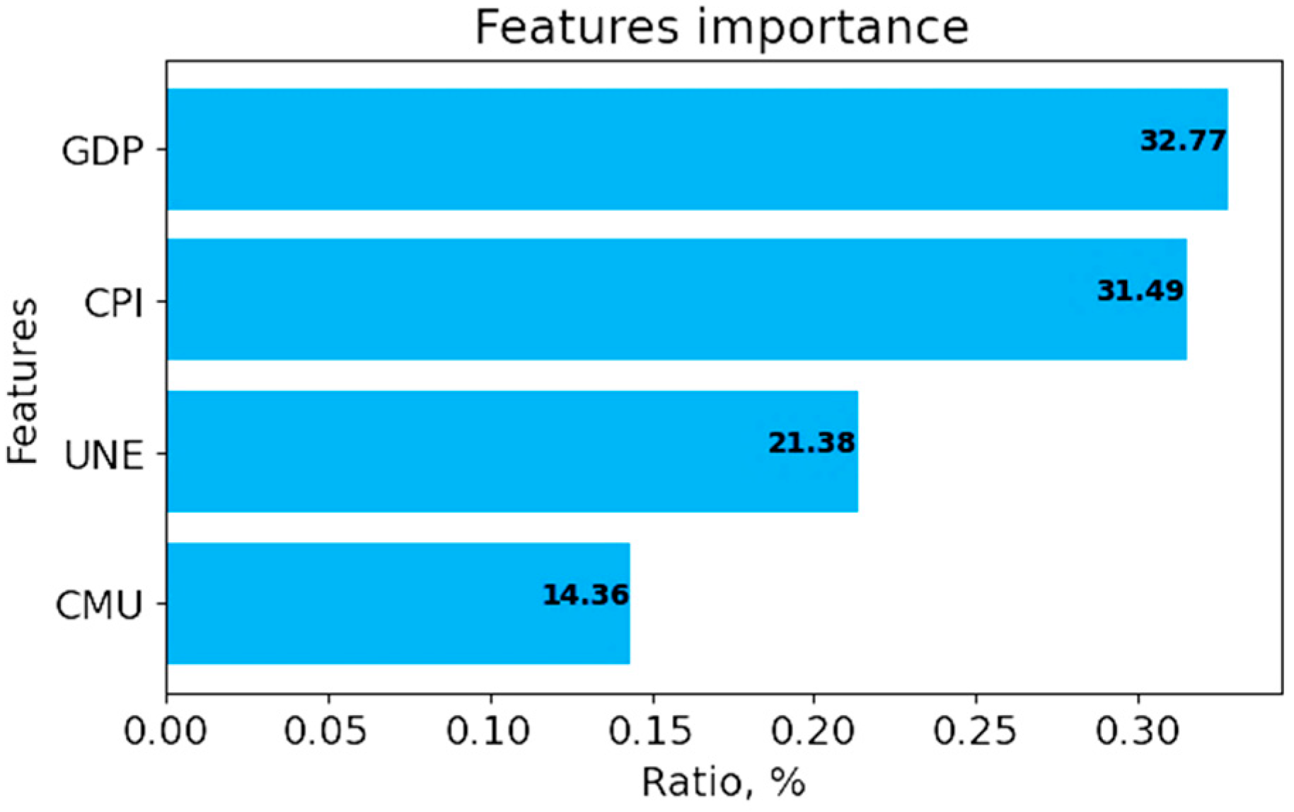
All steps of the ANN evaluations, as well as the selection of the best-performing model, led to the use of the (9, 5) structure with a batch size of 2 for determining the hierarchy of influence of the independent variables on CF, as simulated by the artificial neural network. This hierarchy can be observed in Figure 9.

The bar chart illustrates the relative importance of four independent variables—GDP, CPI, UNE, and CMU—in influencing the dependent variable CF, as determined by the artificial neural network (ANN). The importance is expressed as a percentage ratio:

• GDP has the highest influence at 32.77%,
• Followed closely by CPI at 31.49%,
• UNE (unemployment) contributes 21.38%,
• While CMU has the lowest impact at 14.36%.

The ANN model identifies GDP and CPI as the most influential variables affecting CF, together accounting for over 64% of the total importance showing that economic indicators such as GDP and CPI play a dominant role in shaping the outcome. UNE and CMU, while still relevant, have a comparatively lower impact. This hierarchy of influence supports targeted analysis and decision-making focused primarily on GDP and CPI.

The variable importance in CF evolution training, as determined using the ANN structure 4-9-5-1 (batch size = 2), remains consistent across most of the alternative network architectures and batch sizes applied. The most common deviations from the predominant importance hierarchy (GDP > CPI > UNE > CMU) were of the form CPI > GDP and UNE > CPI, observed in less than 25% of the analyzed cases. Such deviations were primarily noted when using a batch size of 20, as well as in architectures with either a small number of neurons (e.g., 4-3-1 or 4-5-1) or a large number of neurons (e.g., 4-11-7-3-1). These findings reinforce the appropriateness of the chosen structure—both in terms of the number of neurons (4-9-5-1) and the batch size (2)—as deviations from these characteristics tend to disrupt the established importance hierarchy.

4. Discussion and Conclusions

To contextualize Romania’s findings within the broader European landscape, we examined recent studies on the relationship between socioeconomic indicators and environmental impact in other EU countries, notably Italy, Germany, and Spain. These countries have been active in sustainability research and policy implementation, offering valuable benchmarks for comparative analysis.

For instance, ref. [33] analyzed macroeconomic sustainability across European economies and found that green employment and ESG-aligned economic performance significantly contribute to GDP and environmental outcomes. Their study highlights the role of economic indicators such as GDP and employment in advancing SDG targets, particularly SDG 8 (Decent Work and Economic Growth) and SDG 12 (Responsible Consumption and Production).

Similarly, ref. [34] explored the link between economic complexity and ecological footprint in highly developed economies, including Germany and Italy. The study confirmed a positive long-term association between GDP per capita and environmental impact, reinforcing the findings of our ANN model that identified GDP and CPI as dominant drivers of the CF.

These comparative insights validate the applicability of our analytical framework and support the conclusion that economic growth and price dynamics are consistent predictors of consumption-related environmental pressure across diverse EU contexts. They also underscore the importance of integrating labor market and innovation indicators into future models to capture broader sustainability dimensions.

To ensure alignment with global sustainability objectives, each indicator has been mapped to specific Sustainable Development Goals (SDGs):

• GDP → SDG 8 (Decent Work and Economic Growth), reflecting the link between economic performance and sustainable employment. Economic Growth (GDP) drives higher consumption levels, increasing resource use and emissions. Rising GDP typically correlates with greater demand for goods and services, amplifying environmental pressures.
• CPI → SDG 12 (Responsible Consumption and Production), emphasizing the role of price mechanisms in promoting sustainable consumption. CPI affect consumer choices by influencing affordability and substitution patterns. Price fluctuations can shift demand toward products with varying environmental footprints.
• UNE → SDG 10 (Reduced Inequalities), as labor market stability supports equitable access to resources. UNE influence household income and purchasing power, indirectly shaping consumption intensity and sustainability preferences.
• CMU → SDG 12 and SDG 13 (Climate Action), highlighting circularity as a key strategy for reducing emissions and resource depletion. CMU mitigates environmental impact by promoting resource efficiency and reducing dependency on primary raw materials.

This research provides a comprehensive and structured approach to understanding the key factors influencing CF, a central metric in evaluating sustainability within the European Union. By categorizing the 17 SDGs into five thematic clusters—economic conditions, globalization and technology, health, environmental awareness, and cultural factors—the study offers a clear analytical framework that enhances both interpretability and policy relevance.

The methodological rigor of the study is reflected in its dual approach: Graphical representations and correlation analyses and advanced modeling through ANNs, supported by statistical analysis using non-parametric tests (Cronbach’s alpha test, Shapiro-Wilk test, Bartlett’s test, Kruskal–Wallis and Mann–Whitney U). These methods revealed that GDP and CPI are the most influential variables affecting CF, followed by UNE and CMU. The ANN model confirmed this hierarchy, with GDP and CPI together accounting for over 64% of the total influence on CF.

Graphical representations and correlation analyses further supported these findings, showing that GDP and CPI exhibit stable and interpretable relationships with CF, while CMU demonstrates weak and erratic behavior. The study also highlighted the limitations of traditional parametric methods due to data non-normality and heteroscedasticity, reinforcing the value of non-parametric and machine learning techniques in sustainability research.

The interpretation of such a hierarchy can be done as follows: GDP, as the most influential variable, suggests that economic growth directly drives consumption levels, which in turn increase environmental impact. CPI, closely following GDP, indicates that price dynamics affect consumer choices, potentially shifting demand toward more or less sustainable products. The unemployment rate influences purchasing power and social stability, indirectly shaping consumption behavior. CMU, despite its relevance to circular economy practices, shows the least influence, possibly due to limited integration of circularity into mainstream consumption or the indicator’s low sensitivity to short-term changes.

To evaluate the robustness of the findings, a linear regression model (sns.regplot) was implemented using the same dataset and variables (GDP, CPI, UNE, CMU) as those applied in the ANN analysis. The regression model provided a baseline understanding of the linear relationships between the independent variables and CF. While the linear model confirmed the positive association between GDP and CPI with CF, its predictive accuracy was significantly lower compared to the ANN approach.

This limitation stems from the pronounced nonlinearity observed in relationships, particularly for CPI and UNE, as revealed by graphical analysis (Figure 4). Also, the fitted regression lines failed to capture the curvature and variability present in the original data, resulting in higher residual errors and reduced explanatory power. In contrast, the ANN model effectively accommodated these nonlinear patterns, delivering a more accurate simulation and hierarchy of variable importance.

These results underscore the advantage of ANN modeling for complex sustainability datasets, where interactions among socioeconomic indicators and environmental impact cannot be adequately represented by linear assumptions.

To consolidate these observations,

Table 7. Comparative summary of each variable’s influence as determined by both graphical analysis and ANN modeling.

Variable	Correlation Strength	Graphical Pattern	ANN Importance	Interpretation
GDP	High (r > 0.7)	Moderate clustering, stable trend	32.77%	Strong, consistent influence
CPI	High (r > 0.7)	Dense clustering, non-linear	31.49%	Strong, dynamic influence
UNE	Moderate (r > 0.7)	Broad spread, localized density	21.38%	Variable, context-dependent
CMU	Low (r ≈ 0.7)	Dispersed, low density	14.36%	Weak, minimal impact

Source: Authors’ calculation.

presents a comparative summary of each variable’s influence as determined by both graphical analysis and ANN modeling.

This table reinforces the conclusion that GDP and CPI are the most influential drivers of CF, while UNE has a moderate effect and CMU contributes marginally.

Overall, the paper contributes significantly to the field by offering a replicable and adaptable model for analyzing sustainability indicators. Its findings are highly relevant for policymakers, researchers, and practitioners aiming to design targeted interventions that accelerate progress toward the EU’s sustainability objectives. The integration of structured SDG clustering with robust analytical tools positions this work as a valuable reference for future studies in sustainable consumption and development planning.

Also, building on the analytical results, we propose actionable strategies that integrate economic and educational policies to mitigate environmental impact:

• Economic Policies

• Green Taxation and Incentives: Introduce progressive green taxes on high-impact products and services, while offering subsidies for sustainable alternatives. This approach leverages the strong influence of GDP and CPI on consumption patterns.
• Support for Circular Economy: Increase investments in sectors that promote material reuse and recycling, thereby enhancing CMU and reducing resource extraction.
• Price Regulation for Sustainable Goods: Implement price stabilization mechanisms for eco-friendly products to counteract CPI volatility and encourage sustainable purchasing behavior.

• Educational Policies

• Curriculum Integration: Embed sustainability principles and circular economy concepts into school and university curricula to foster long-term behavioral change.
• Awareness Campaigns: Launch nationwide campaigns emphasizing the environmental cost of consumption and practical steps for reducing CF.
• Community-Based Programs: Promote local initiatives such as repair cafés, recycling workshops, and sustainability clubs to strengthen cultural norms around responsible consumption.

These recommendations are aligned with SDG 12 (Responsible Consumption and Production) and aim to translate analytical insights into actionable strategies for policymakers. By targeting both economic levers and educational interventions, these measures address the dominant drivers of CF while fostering systemic behavioral change

The study’s limitations are a result of the fact that study is based on data from Romania between 2012 and 2023, which, while relevant, may not capture long-term trends or broader regional dynamics. The application of ANNs in this study was exploratory in nature, aimed at complementing traditional statistical methods and identifying potential nonlinear relationships among sustainability indicators. To mitigate the risk of overfitting, several safeguards were implemented, including the use of regularization techniques, careful selection of network architecture, and validation through testing accuracy. The training and testing errors were consistently low, and the model’s predictions closely matched actual values, suggesting that the ANN captured meaningful patterns despite the limited data. Furthermore, the consistency of results across statistical and AI-based methods reinforces the robustness of the findings. While we agree that larger datasets are preferable for generalization, the current approach provides valuable preliminary insights and a foundation for future research with expanded data.

Future research could expand the dataset to include multiple countries, longer time series, and behavioral data. Moreover, integrating explainable AI techniques and dynamic modeling could enhance the interpretability and predictive power of the framework. These improvements would support more targeted and effective sustainability strategies aligned with the SDGs. Moreover, incorporating longitudinal data and analyzing the effects of policy interventions would strengthen the validation of the causal relationships suggested by the ANN-derived hierarchy.

References

1. Peng, C.; Law, Y.-W. How Do Consumption Patterns Influence the Discrepancy Between Economic and Subjective Poverty? J. Happiness Stud. 2023, 24, 1579–1604. [Google Scholar] [CrossRef]
2. Cleveland, M. Globalization and global consumer culture: The fragmentation, fortification, substitution and transmutation of social identities. In Globalized Identities: The Impact of Globalization on Self and Identity; Katzarska-Miller, I., Reysen, S., Eds.; Palgrave Macmillan: London, UK, 2022; pp. 71–105. ISBN 978-3-031-04644-5. [Google Scholar] [CrossRef]
3. Melumad, S.; Hadi, R.; Hildebrand, C.; Ward, A. Technology-augmented choice: How digital innovations are transforming consumer decision processes. Cust. Needs Solut. 2020, 7, 90–101. [Google Scholar] [CrossRef]
4. Liu, Y.; Lopez, R.A. The impact of social media conversations on consumer brand choices. Mark. Lett. 2016, 27, 1–13. [Google Scholar] [CrossRef]
5. García-Salirrosas, E.E.; Esponda-Perez, J.A.; Millones-Liza, D.Y.; Haro-Zea, K.L.; Moreno-Barrera, L.A.; Ezcurra-Zavaleta, G.A.; Rivera-Echegaray, L.A.; Escobar-Farfan, M. The influence of healthy lifestyle on willingness to consume healthy food brands: A perceived value perspective. Foods 2025, 14, 213. [Google Scholar] [CrossRef] [PubMed]
6. Testa, F.; Pretner, G.; Iovino, R.; Bianchi, G.; Tessitore, S.; Iraldo, F. Drivers to green consumption: A systematic review. Environ. Dev. Sustain. 2020, 23, 4826–4850. [Google Scholar] [CrossRef]
7. Rahman, S.U.; Chwialkowska, A.; Hussain, N.; Bhatti, W.A.; Luomala, H. Cross-cultural perspective on sustainable consumption: Implications for consumer motivations and promotion. Environ. Dev. Sustain. 2023, 25, 997–1016. [Google Scholar] [CrossRef]
8. Gross Domestic Product. Available online: https://ec.europa.eu/eurostat/databrowser/view/tec00114/default/table?lang=en&category=t_na10.t_nama10.t_nama_10_ma (accessed on 15 January 2025).
9. Price Level Indices. Available online: https://ec.europa.eu/eurostat/databrowser/view/tec00120__custom_15072228/default/table?lang=enc (accessed on 15 January 2025).
10. Antohi, I.; Ghiță-Mitrescu, S. NEETs’ Attitude towards Entrepreneurship. Ovidius Univ. Ann. Ser. Econ. 2022, 22, 498–506. [Google Scholar] [CrossRef]
11. Unemployment Rate by Sex. Available online: https://ec.europa.eu/eurostat/databrowser/view/tesem120/default/table?lang=en&category=es.tesem (accessed on 15 January 2025).
12. KOF Globalisation Index. Available online: https://ts-explorer.kof.ethz.ch/guest/941475d6-b1bb-462d-985f-2dee0f4fcc04?range=0-50 (accessed on 15 January 2025).
13. Healthy Life Years. Available online: https://ec.europa.eu/eurostat/databrowser/view/tps00150__custom_15073772/default/table?lang=en (accessed on 15 January 2025).
14. Share of Renewable Energy in Gross Final Energy Consumption. Available online: https://ec.europa.eu/eurostat/databrowser/view/sdg_07_40/default/table?lang=en&category=sdg.sdg_13 (accessed on 15 January 2025).
15. Ghiță-Mitrescu, S. Mapping Romania’s progress towards a circular economy using the EU Circular Economy Monitoring Framework. Ovidius Univ. Ann. Ser. Civ. Eng. 2024, 26, 156–164. [Google Scholar] [CrossRef]
16. Circular Material Use Rate. Available online: https://ec.europa.eu/eurostat/databrowser/view/sdg_12_41/default/table?lang=en&category=sdg.sdg_12 (accessed on 15 January 2025).
17. Persons Employed in Circular Economy Sectors. Available online: https://ec.europa.eu/eurostat/databrowser/view/cei_cie011__custom_15073943/default/table?lang=en (accessed on 1 June 2025).
18. Consumption Footprint—Single Weighted Score. Available online: https://ec.europa.eu/eurostat/databrowser/view/sdg_12_31/default/table?lang=en&category=sdg.sdg_12 (accessed on 15 January 2025).
19. seaborn.lineplot. Available online: https://seaborn.pydata.org/generated/seaborn.lineplot.html (accessed on 1 June 2025).
20. seaborn.jointplot. Available online: https://seaborn.pydata.org/generated/seaborn.jointplot.html (accessed on 1 June 2025).
21. sns.regplot. Available online: https://weisscharlesj.github.io/SciCompforChemists/notebooks/chapter_10/chap_10_notebook.html (accessed on 1 June 2025).
22. Corrmat. Available online: https://www.geeksforgeeks.org/create-a-correlation-matrix-using-python/ (accessed on 13 July 2025).
23. curve_fit. Available online: https://docs.scipy.org/doc/scipy/reference/generated/scipy.optimize.curve_fit.html (accessed on 13 July 2025).
24. ax.plot_surface. Available online: https://matplotlib.org/stable/api/_as_gen/mpl_toolkits.mplot3d.axes3d.Axes3D.plot_surface.html (accessed on 13 July 2025).
25. np.polyfit. Available online: https://numpy.org/doc/stable/reference/generated/numpy.polyfit.html (accessed on 13 July 2025).
26. Pedregosa, F.; Varoquaux, G.; Gramfort, A.; Michel, V.; Thirion, B.; Grisel, O.; Duchesnay, É. Scikit-learn: Machine learning in Python. J. Mach. Learn. Res. 2011, 12, 2825–2830. [Google Scholar]
27. Relu Function. Available online: https://keras.io/2/api/layers/activations/ (accessed on 13 July 2025).
28. Tanh. Hyperbolic Tangent. Available online: https://www.mathworks.com/help/matlab/ref/double.tanh.html (accessed on 13 July 2025).
29. Adam. Available online: https://keras.io/api/optimizers/adam/ (accessed on 13 July 2025).
30. Stochastic Gradient Descent. Available online: https://scikit-learn.org/stable/modules/sgd.html (accessed on 13 July 2025).
31. Batch Size in Neural Network. Available online: https://www.geeksforgeeks.org/deep-learning/batch-size-in-neural-network/ (accessed on 13 July 2025).
32. Regression Metrics. Available online: https://www.geeksforgeeks.org/machine-learning/regression-metrics/ (accessed on 13 July 2025).
33. Figuerola-Ferretti, I.; Lumbreras, S.; Paraskevas, P.; Paraskevopoulos, I. Sustainability in action: Macro-level evidence from Europe (2008–2023) on ESG, green employment, and SDG-aligned economic performance. Sustainability 2025, 17, 9103. [Google Scholar] [CrossRef]
34. Neagu, O. Economic complexity and ecological footprint: Evidence from the most complex economies in the world. Sustainability 2020, 12, 9031. [Google Scholar] [CrossRef]
35. Cronbach, L.J. Coefficient alpha and the internal structure of tests. Psychometrika 1951, 16, 297–334. [Google Scholar] [CrossRef]
36. Shapiro, S.S.; Wilk, M.B. An analysis of variance test for normality (complete samples). Biometrika 1965, 52, 591–611. [Google Scholar] [CrossRef]
37. Reddon, J.R.; Jackson, D.N. A note on testing the sphericity hypothesis with Bartlett’s test. Multivar. Exp. Clin. Res. 1984, 7, 49–52. [Google Scholar] [CrossRef]
38. Kruskal, W.H.; Wallis, W.A. Use of ranks in one-criterion variance analysis. J. Am. Stat. Assoc. 1952, 47, 583–621. [Google Scholar] [CrossRef]
39. Mann, H.B.; Whitney, D.R. On a test of whether one of two random variables is stochastically larger than the other. Ann. Math. Stat. 1947, 18, 50–60. [Google Scholar] [CrossRef]
Figure 1. CF correlations according to: (a) all independent variables; (b) 4 independent variables with corr > 0.7. Source: Authors’ graphic representation.
Systems 13 01022 g001
Figure 2. Examples of ANNs’ structures: (a) 4-7-1; (b) 4-9-3-1; (c) 4-11-5-3-1 layers (hidden layers and hidden neurons). Source: Authors’ graphic representation.
Systems 13 01022 g002
Figure 3. CF scatter values (clouds of data) in accordance with the values of the independent variables: (a) GDP; (b) CPI; (c) UNE; (d) CMU; using Joinplot. Source: Authors’ graphic representation.
Systems 13 01022 g003
Figure 4. CF’s dispersion, trend and fitted values in accordance with the values of the independent variables: (a) GDP; (b) CPI; (c) UNE; (d) CMU; using Polyfit and regplot. Source: Authors’ graphic representation.
Systems 13 01022 g004aSystems 13 01022 g004b
Figure 5. 3D surfaces of CF against: (a) GDP & CPI; (b) GDP & UNE; (c) GDP & CMU; (d) UNE & CPI; (e) CPI & CMU; (f) UNE & CMU. Source: Authors’ graphic representation.
Systems 13 01022 g005aSystems 13 01022 g005b
Figure 6. MLP Train performance (here only for ReLU with Adam optimizer): (a) train_mae; (b) train_mse; (c) test_mae; (d) test_mse. Source: Authors’ graphic representation.
Systems 13 01022 g006
Figure 7. Network error curve. Source: Authors’ calculation.
Systems 13 01022 g007
Figure 8. Target vs. simulated values. Source: Authors’ calculation.
Systems 13 01022 g008
Figure 9. Variable’s importance on CF evolution training. Source: Authors’ graphic representation.
Systems 13 01022 g009