A Hybrid Modeling Framework for Evaluating ESG Investment Risks in Highway Real Estate Investment Trusts: Insights from Chinese Highway Assets

Abstract

ESG (Environmental, Social, and Governance) considerations are increasingly influencing REIT (real estate investment trust) investment decisions; however, empirical evidence on the ESG–financial performance nexus in infrastructure REITs remains scarce. Given China’s nascent highway REIT market, this exploratory study proposes a hybrid modeling framework that integrates static econometric analysis with dynamic system simulation to examine how ESG factors affect investment risk. Using VaR (Value at Risk) analysis and an ESG-adjusted CAPM (Capital Asset Pricing Model) on 10 Chinese highway REITs (2021Q2–2025Q2), we constructed a composite ESG indicator via a weighted proxy approach. We identified three key findings testing hypotheses linked to ESG finance theory; these findings support H1 (non-monotonic VaR reduction) and partially confirm H2 (inverted-U path with lag): (1) the ESG-adjusted weighted average cost of capital (WACC) exhibits an inverted U-shaped trajectory with post-peak oscillations and an overall 20-month implementation lag (derived from system dynamics simulations) to efficiency realization; (2) the results suggest initial evidence showing that an ESG investment intensity (IEP ≈ 0.40, representing moderate ESG resource allocation) may indicate potential outperformance over both under-investment (−5.0% deviation in risk-adjusted returns) and over-investment (−8.0% deviation in risk-adjusted returns), though with uncertainty in static estimates; and (3) system dynamics validation suggests potential predictive accuracy. These preliminary findings challenge linear ESG–performance assumptions and offer dynamic risk assessment tools; nevertheless, as an exploratory study, they warrant replication in larger and more diverse samples. Thus, the results should be regarded as preliminary guidance rather than conclusive evidence, with further validation needed to confirm generalizability.

1. Introduction

Highway infrastructure REITs face increasing ESG-related economic risks. Environmental concerns have raised the weighted-average cost of capital (WACC) and heightened volatility, with the Global Infrastructure Hub forecasting a USD 20 trillion investment shortfall by 2040 [1]. While ESG regulations may increase short-term O&M expenses, they promise long-term efficiency gains [2].

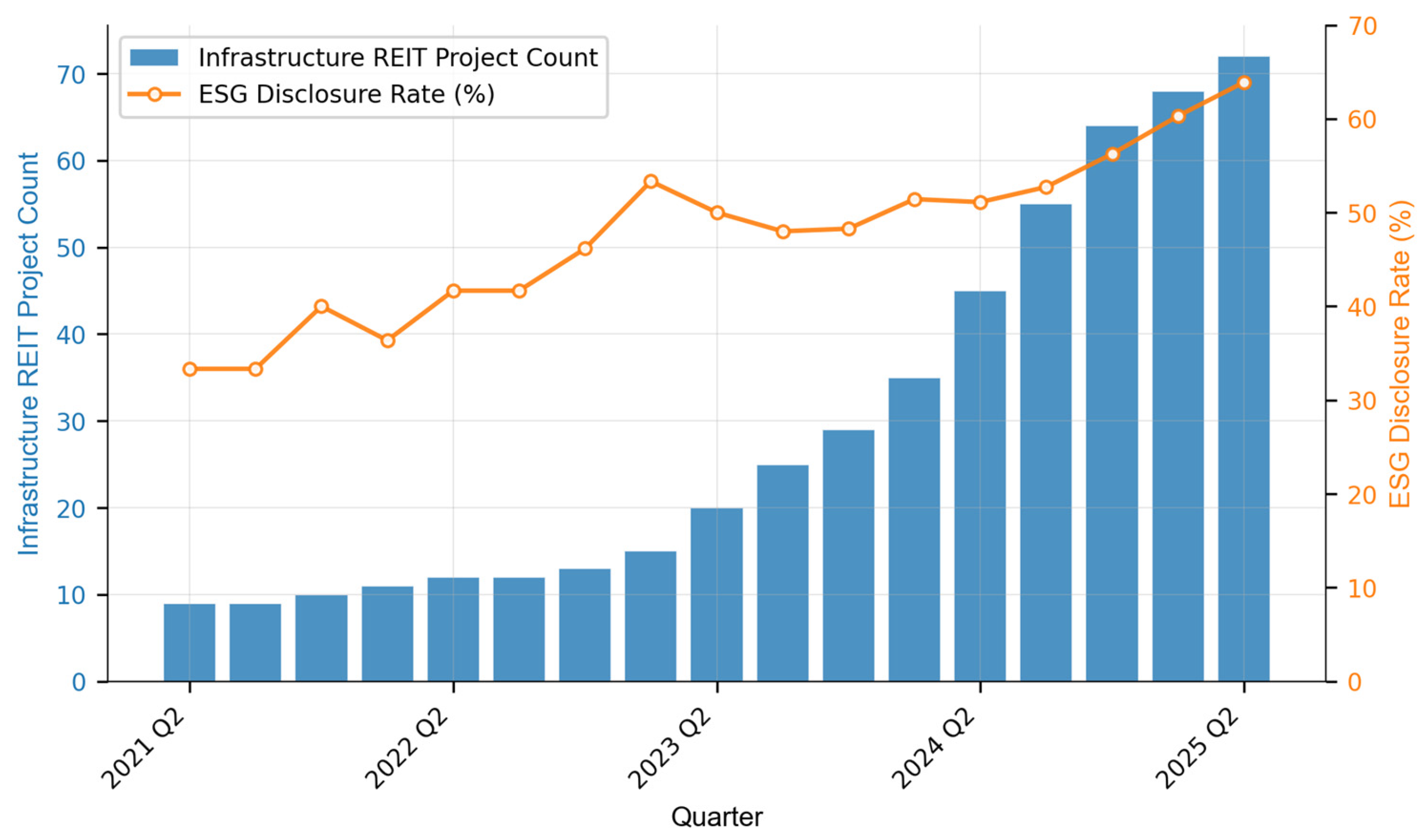
Empirical evidence on ESG–REIT relationships remains inconclusive, with studies finding negative short-term [3,4] versus null or positive long-term effects [5]. Figure 1 shows the concurrent growth in Chinese highway REIT projects and ESG disclosure rates. Given the nascent nature of China’s highway REIT market (launched in 2021) and the limited sample of infrastructure REITs available, this study adopted an exploratory research approach to provide initial insights into ESG–risk relationships in this emerging asset class.

Figure 1. Trends in ESG disclosure and infrastructure REIT project launches in China. Data compiled from Wind and CSMAR.

Previous studies using static metrics (VaR, ESG-adjusted CAPM) overlooked temporal dynamics and non-linear feedback mechanisms. While considering system dynamics has proven valuable in energy and supply chain contexts [6,7], its application to highway REITs remains limited.

This study addresses these gaps by combining static econometric analysis with dynamic system simulation. Specifically, we quantified ESG-adjusted VaR relationships in static settings, simulated dynamic trajectories of REIT using system dynamics models, and investigated ESG investment intensity patterns to identify potentially advantageous ranges around IEP = 0.40 that may improve risk-adjusted returns while avoiding both under- and over-investment inefficiencies. Theoretically, this research provides initial evidence suggesting the presence of more intricate temporal ESG–finance relationships beyond simplistic linear assumptions. Methodologically, it demonstrates a high level of predictive consistency in system dynamics modeling (r = 0.894, p < 0.001) while recognizing the exploratory nature of the findings. Practically, it offers preliminary guidance for REIT managers regarding the prioritization of ESG investment calibration strategies, although broader validation is warranted.

The remainder of this paper is organized as follows: Section 2 reviews the relevant literature on ESG integration, infrastructure risks, and system dynamics applications; Section 3 presents the hybrid modeling framework and methodology; Section 4 reports empirical results from the static analysis, dynamic simulation, and model validation; Section 5 discusses the theoretical implications, methodological contributions, and strategic insights; and Section 6 concludes with findings, limitations, and future research directions. Furthermore, based on the identified literature gaps, to guide this exploratory study, we propose the following prior hypotheses: H1—A higher IEP is expected to reduce VaR, exhibiting non-monotonic patterns (e.g., based on ESG risk dynamics in emerging markets). H2—ESG-adjusted WACC is expected to follow an inverted-U non-monotonic trajectory with an implementation lag. Analytically, H1 extends VaR with quadratic terms; H2 integrates CAPM with dynamics for feedback, linking to mainstream ESG theory. Moreover, the two hypotheses link the aims of quantifying ESG’s effects on risk to the hybrid methods and conclusions on temporal dynamics.

2. Literature Review

Previous studies examined ESG-related economic risks in highway REITs across sustainable finance, real estate economics, and system dynamics modeling. This review identifies patterns in ESG–finance relationships and highlights gaps in integrating static and dynamic methodologies.

2.1. ESG Integration and Financial Performance in REITs

Research indicates that ESG considerations affect REIT returns and volatility primarily by enhancing governance and sustainability practices. Bauer et al. found that robust board structures and stakeholder alignment increase the operational efficiency and decrease agency costs [8]. Eichholtz demonstrated that environmental ESG factors boost property values and mitigate energy-related risks through green building certifications [9].

Liu et al. applied the Hurst exponent to evaluate the Hong Kong REIT market efficiency, revealing lasting correlations, where ESG compliance enhances market stability [10]. Their subsequent analysis of Chinese REITs using time-varying parameter vector autoregression models showed that ESG-aligned REITs alleviate systemic financial spillovers during volatility periods [11]. Chen et al. found that ESG factors influence cash flow multipliers and risk premiums in infrastructure assets, such as hydropower stations [12].

Meta-analyses support these trends. Friede et al. synthesized over 2000 studies, determining that ESG integration generally leads to favorable risk-adjusted returns, particularly emphasizing social and governance aspects in REIT settings [13]. Erol et al., utilizing panel data from mature REIT markets, observed that ESG investments enhance financial outcomes, especially during periods of heightened market volatility [14]. Shangguan et al. documented a curvilinear relationship between ESG performance and firm value in the Chinese context [15].

These studies indicate that ESG integration enhances financial resilience in REITs, with variations stemming from market-specific conditions and sectoral emphasis.

2.2. Economic Risks in Highway Infrastructure Projects

Economic risks in highway infrastructure projects involve cost overruns, financing difficulties, and operational uncertainties often associated with ESG factors. Song et al. utilized decision-making trials and evaluated laboratory-interpretive structural modeling to assess social risks in rail transit projects, emphasizing stakeholder resistance and environmental consequences as sources of economic instability [16]. Lv et al. expanded this methodology to highway REITs, delineating 15 risk factors where ESG non-compliance exacerbated uncertainties [17].

Wang et al. reviewed China’s public–private partnership frameworks, highlighting governance mechanisms that enhance risk allocation efficiency [18]. Zhang et al. analyzed public–private partnership research, stressing the importance of enhanced risk sharing in infrastructure projects to mitigate financial risks [19]. Maqsoom et al. explored construction risks in highway development, revealing that social sustainability moderates cost overruns [20]. Engineering and managerial viewpoints provide additional insight. Deep et al. pinpointed key performance indicators in highway systems, including complexity and challenges with subcontractors, which amplify financial losses [21]. Kashyap and Sharma examined infrastructure investment trusts as a funding mechanism, highlighting ESG considerations’ role in attracting investment during high-interest-rate periods [22]. Han developed a risk assessment model for pipeline corridors, with implications for highways, revealing the non-linear nature of ESG-related risks [23].

Research highlights the interrelated economic vulnerabilities in highway projects shaped by environmental regulations and social responsibility factors.

2.3. System Dynamics Applications in Risk Management and Sustainability

System dynamics (SD) modeling analyzes complex risks within infrastructure and sustainability domains, simulating feedback loops and non-linear interactions. Sterman established fundamental SD principles in business dynamics, highlighting its utility in modeling economic and environmental systems [24]. Hjorth and Bagheri extended SD applications to sustainable development, showcasing adaptive strategies for resource management [25].

Nguyen et al. applied SD in infrastructure contexts to assess the socioeconomic advantages of transportation projects [26]. Ghufran et al. analyzed circular economy facilitators in the construction sector, delineating feedback loops that impact sustainability risks [27]. Xue et al. formulated an SD model to evaluate risk interactions in high-speed rail projects, quantifying uncertainty amplification [28]. Jonsdottir et al. examined the integration of sustainable development (SD) principles into business strategies, emphasizing its significance in ESG transitions [29]. Sánchez-García et al. developed a model to assess organizational resilience in small- and medium-sized enterprises, demonstrating the effectiveness of SD in capturing the dynamic impacts of ESG factors [30]. Yuan and Yang conducted an evaluation of cross-border transportation systems using SD, emphasizing the importance of mitigating risks through the integration of various factors [31]. Martinez-Moyano and Richardson proposed best practices for system dynamics (SD), recommending hybrid models for complex scenarios [32]. Their work showcases the adaptability of SD in analyzing risk dynamics in financial, environmental, and managerial contexts.

These applications demonstrate SD’s effectiveness at capturing dynamic ESG factors’ impacts in financial, environmental, and managerial contexts.

In summary, existing literature highlights ESG integration’s positive impact on REIT financial performance [8,13], diverse ESG factors influencing economic risks in highway projects [17], and SD modeling’s efficacy at capturing complex interactions [24,26].

However, recent REIT–ESG meta-studies indicate mixed evidence on financial performance, with influences from environmental and social pillars but limited dynamic analysis in emerging contexts [14]. Specifically, China-specific ESG regulation timelines provide crucial context: the 2021 CSRC REIT pilot program initiated ESG considerations [33], followed by 2022 guidelines emphasizing disclosure [34] and 2024 SSE mandates for mandatory ESG reporting in infrastructure assets [35]. Moreover, these developments highlight regulatory evolution, yet gaps persist in integrating static risk metrics with temporal simulations for highway REITs.

Given these developments, a critical synthesis reveals inconsistencies in prior ESG–finance summaries. For instance, mature markets often report positive long-term ESG effects [14]. In contrast, emerging contexts such as China show mixed or negative short-term impacts due to implementation costs [15]. These inconsistencies underscore the need for non-linear models over linear assumptions, as explored in our hypotheses (H1 on non-monotonic VaR reduction and H2 on inverted-U WACC paths). Methodologically, gaps include overreliance on static metrics, such as VaR/CAPM ignoring feedback loops, and SD applications limited to non-REIT sectors [27,28]. Overall, this highlights the absence of hybrid approaches that integrate cross-sectional risk benchmarks with temporal simulations. Such gaps may overestimate ESG benefits in dynamic infrastructure settings. Therefore, our study explores this through an exploratory hybrid framework. It synthesizes these streams and suggests preliminary non-monotonic patterns. These warrant further empirical validation in larger samples.

3. Methodology

3.1. Design Overview

This research employed an exploratory methodology due to the inherent limitations of China’s newly established highway REIT market. With 10 highway REITs available since market inception in 2021Q2, our study aims to establish preliminary empirical patterns and theoretical frameworks for future large-sample validation. We employed a sequential mixed-methods design that transitions from static, cross-sectional calibration to longitudinal system dynamics simulation [36]. The process involved data preparation, static risk estimation, system dynamic modeling, integration, and validation, following established protocols in sustainable finance system dynamics studies [23,37,38]. This sequential mixed-methods design was guided by the prior hypotheses stated in Section 1: the static VaR and CAPM analyses provided preliminary tests for H1 (IEP’s expected non-monotonic effects on VaR), while the dynamic SD simulation examined H2 (non-monotonic WACC path with implementation lag). Figure 2 provides an overview of the analytical workflow.

Figure 2. Analytical pipeline.

3.2. Data Sources and Sample Construction

3.2.1. Sampling Frame

The sample consisted of all publicly traded Chinese toll-highway REITs (2021Q2–2025Q2) meeting three criteria: market capitalization ≥ CNY 2 billion, continuous trading ≥ 18 months, and available ESG disclosures. This yielded 10 REITs with 210 REIT-month observations, with over 2000 variable instances variable-time observations for robust statistical analysis.

3.2.2. Data Streams

Data from various channels were collected to encompass financial, operational, and ESG metrics, which ensured a comprehensive ESG–VaR analysis. Table 1 provides an overview of the primary sources and their respective scopes.

Table 1. Data sources, variables, and processing methods for highway REIT analysis (2021Q2–2025Q2).

Source	Variables	Processing Details	Data Frequency and Notes
Wind and CSMAR	Closing price, trading volume, net asset value (NAV), distributions	Winsorized at 1%/99% levels (removing ~2% outliers to reduce extreme value impact).	Daily
Issuer filings	Toll revenue, operation and maintenance (O&M) costs, capital expenditures (capex), leverage	Linear interpolation for ≤ 3 months missing; gaps > 3 months flagged for exclusion if exceeding 5% threshold.	Monthly/quarterly (converted to monthly)
CSR/ESG reports/issuer filings	Environmental, Social, and Governance performance	Min–max normalization within each month.	Monthly/quarterly (converted to monthly)
Macro sources	10-year bond yield, Brent crude oil price, Gross Domestic Product (GDP)	Cross-source reconciliation (e.g., averaging from multiple databases for consistency).	Monthly

Note: Missing values (<5% for all sources) were handled using linear interpolation unless otherwise specified.

Data cleaning resulted in 210 observations for VaR analysis and 186 for ESG–CAPM analysis after excluding cases with insufficient market data (12), incomplete ESG variables (8), and regulatory inconsistencies (4). The 2025 Q2 timeframe refers to data disclosed up to the end of June 2025, primarily based on monthly operational reports, with quarterly and semi-annual reports serving as supplements. For the detailed CONSORT-style flow and methodological rationale, see Appendix A (Table A1 and Table A2).

3.3. Variable Definitions and Construction

3.3.1. ESG Proxy Construction and Methodology

Due to limited direct ESG expenditure disclosure in China’s infrastructure REIT market, we constructed an investment in ESG performance (IEP) composite using proxy variables following established practices [13].

The ESG proxy index (IEP) adopts equal weights across environmental (E), social (S), and governance (G) dimensions (1/3 each). Given the small sample, we adopted equal weighting per OECD guidelines [39], rather than data-driven methods; this approach is applied when expert consensus is lacking, ensuring transparency and objectivity without introducing subjective biases.

The Environmental dimension (E) combines resource efficiency and asset utilization, as measured using the following equations with equal weights [40]:

$$\mathrm{R}\mathrm{e}\mathrm{s}\mathrm{o}\mathrm{u}\mathrm{r}\mathrm{c}\mathrm{e} \mathrm{E}\mathrm{f}\mathrm{f}\mathrm{i}\mathrm{c}\mathrm{i}\mathrm{e}\mathrm{n}\mathrm{c}\mathrm{y}=\mathrm{T}\mathrm{o}\mathrm{l}\mathrm{l} \mathrm{R}\mathrm{e}\mathrm{v}\mathrm{e}\mathrm{n}\mathrm{u}\mathrm{e}/\mathrm{M}\mathrm{a}\mathrm{i}\mathrm{n} \mathrm{O}\mathrm{p}\mathrm{e}\mathrm{r}\mathrm{a}\mathrm{t}\mathrm{i}\mathrm{n}\mathrm{g} \mathrm{C}\mathrm{o}\mathrm{s}\mathrm{t}\mathrm{s}$$

(1)

$$\mathrm{A}\mathrm{s}\mathrm{s}\mathrm{e}\mathrm{t} \mathrm{U}\mathrm{t}\mathrm{i}\mathrm{l}\mathrm{i}\mathrm{z}\mathrm{a}\mathrm{t}\mathrm{i}\mathrm{o}\mathrm{n}=\mathrm{T}\mathrm{o}\mathrm{l}\mathrm{l} \mathrm{R}\mathrm{e}\mathrm{v}\mathrm{e}\mathrm{n}\mathrm{u}\mathrm{e}/\mathrm{T}\mathrm{o}\mathrm{t}\mathrm{a}\mathrm{l} \mathrm{A}\mathrm{s}\mathrm{s}\mathrm{e}\mathrm{t}\mathrm{s}$$

(2)

The Social dimension (S) captures investor welfare, measured as distributable income per unit, and service stability (weighted 0.6 and 0.4, respectively), proxied as the equations below [41]:

$$\mathrm{I}\mathrm{n}\mathrm{v}\mathrm{e}\mathrm{s}\mathrm{t}\mathrm{o}\mathrm{r} \mathrm{W}\mathrm{e}\mathrm{l}\mathrm{f}\mathrm{a}\mathrm{r}\mathrm{e}=\mathrm{D}\mathrm{i}\mathrm{s}\mathrm{t}\mathrm{r}\mathrm{i}\mathrm{b}\mathrm{u}\mathrm{t}\mathrm{a}\mathrm{b}\mathrm{l}\mathrm{e} \mathrm{A}\mathrm{m}\mathrm{o}\mathrm{u}\mathrm{n}\mathrm{t}/\mathrm{U}\mathrm{n}\mathrm{i}\mathrm{t}\mathrm{s} \mathrm{O}\mathrm{u}\mathrm{t}\mathrm{s}\mathrm{t}\mathrm{a}\mathrm{n}\mathrm{d}\mathrm{i}\mathrm{n}\mathrm{g}$$

(3)

$$\mathrm{S}\mathrm{e}\mathrm{r}\mathrm{v}\mathrm{i}\mathrm{c}\mathrm{e} \mathrm{S}\mathrm{t}\mathrm{a}\mathrm{b}\mathrm{i}\mathrm{l}\mathrm{i}\mathrm{t}\mathrm{y}=\mathrm{T}\mathrm{r}\mathrm{a}\mathrm{f}\mathrm{f}\mathrm{i}\mathrm{c} \mathrm{A}\mathrm{v}\mathrm{e}\mathrm{r}\mathrm{a}\mathrm{g}\mathrm{e} \mathrm{D}\mathrm{a}\mathrm{i}\mathrm{l}\mathrm{y}/\mathrm{M}\mathrm{e}\mathrm{a}\mathrm{n} \mathrm{T}\mathrm{r}\mathrm{a}\mathrm{f}\mathrm{f}\mathrm{i}\mathrm{c} \mathrm{A}\mathrm{c}\mathrm{r}\mathrm{o}\mathrm{s}\mathrm{s} \mathrm{A}\mathrm{l}\mathrm{l} \mathrm{R}\mathrm{E}\mathrm{I}\mathrm{T}\mathrm{s}$$

(4)

The Governance dimension (G) is measured by financial discipline [42], defined as the following:

$$\mathrm{F}\mathrm{i}\mathrm{n}\mathrm{a}\mathrm{n}\mathrm{c}\mathrm{i}\mathrm{a}\mathrm{l} \mathrm{D}\mathrm{i}\mathrm{s}\mathrm{c}\mathrm{i}\mathrm{p}\mathrm{l}\mathrm{i}\mathrm{n}\mathrm{e}=\left[\right(\mathrm{T}\mathrm{o}\mathrm{l}\mathrm{l} \mathrm{R}\mathrm{e}\mathrm{v}\mathrm{e}\mathrm{n}\mathrm{u}\mathrm{e}-\mathrm{M}\mathrm{a}\mathrm{i}\mathrm{n} \mathrm{O}\mathrm{p}\mathrm{e}\mathrm{r}\mathrm{a}\mathrm{t}\mathrm{i}\mathrm{n}\mathrm{g} \mathrm{C}\mathrm{o}\mathrm{s}\mathrm{t}\mathrm{s}-\mathrm{A}\mathrm{d}\mathrm{m}\mathrm{i}\mathrm{n} \mathrm{E}\mathrm{x}\mathrm{p}\mathrm{e}\mathrm{n}\mathrm{s}\mathrm{e})/\mathrm{F}\mathrm{i}\mathrm{n}\mathrm{a}\mathrm{n}\mathrm{c}\mathrm{i}\mathrm{a}\mathrm{l} \mathrm{E}\mathrm{x}\mathrm{p}\mathrm{e}\mathrm{n}\mathrm{s}\mathrm{e}]\times (1-\mathrm{D}\mathrm{e}\mathrm{b}\mathrm{t} \mathrm{R}\mathrm{a}\mathrm{t}\mathrm{i}\mathrm{o})$$

(5)

Each sub-indicator was normalized within each month using min–max scaling, and the composite IEP score was calculated as the arithmetic mean of the three dimensions.

3.3.2. Value at Risk

Value at Risk (VaR) represents the maximum anticipated loss within a one-month timeframe at a 95% confidence level. Monthly logarithmic returns are calculated as the natural logarithm of the ratio of the current price to the previous price using market data. Historical VaR is determined as the 5th percentile of observed returns using expanding windows. We also computed the parametric VaR, defined as the mean minus 1.645 times the standard deviation, and the conditional VaR for robustness. VaR served as the dependent variable, with IEP as the primary predictor. Quadratic specifications examine potential non-linear relationships. The control variables included GDP growth, Brent oil prices, CN10Y (China 10-Year Government Bond), and debt ratios. REIT and time fixed effects controlled for unobserved heterogeneity. Missing values (<5% for all sources) were handled exclusively by linear interpolation (with a maximum span of 3 months) to preserve temporal continuity and avoid overfitting in the small sample (N = 210); pattern matching (e.g., k-NN imputation) was avoided to minimize the potential bias in non-stationary REIT metrics. All variables were winsorized at the 1st and 99th percentiles (e.g., VaR trimmed from −0.15 to 0.15, affecting ~2% of observations) after imputation but before exclusions, to manage outliers while preserving 98% of the data’s original distribution. This framework facilitated the estimation of the relationship between IEP and VaR using the following equation:

$${\mathrm{V}\mathrm{a}\mathrm{R}}_{it}=\alpha +\delta \times {\mathrm{I}\mathrm{E}\mathrm{P}}_{it}^2+\gamma \times {\mathrm{I}\mathrm{E}\mathrm{P}}_{it}+\beta \prime {\mathrm{C}\mathrm{o}\mathrm{n}\mathrm{t}\mathrm{r}\mathrm{o}\mathrm{l}\mathrm{s}}_{it}+{\mu }_i+{\lambda }_t+{ϵ}_{it}$$

(6)

In this context, δ assesses quadratic effects, γ represents the linear coefficient, ${\mu }_i$ signifies REIT fixed effects, ${\lambda }_t$ indicates time fixed effects, and α denotes the intercept.

3.3.3. ESG-Adjusted CAPM Variables

The ESG-adjusted CAPM extended traditional CAPM by incorporating ESG risk premiums. Excess return (REIT return minus CN10Y yield) served as the dependent variable. Market beta coefficients were estimated through 24-month rolling OLS regressions against Shanghai–Shenzhen 300 excess returns. IEP was included in linear and quadratic forms, with variables centered around means (IEP_c) for interpretation. The model included macroeconomic controls and REIT/time fixed effects.

The empirical model specification was as follows:

$${\mathrm{Excess}\text{\_}\mathrm{Return}}_{it}=\alpha +{\beta }_i\times {\mathrm{Market}\text{\_}\mathrm{Premium}}_t+\lambda \times {\mathrm{I}\mathrm{E}\mathrm{P}}_{it}+\theta \times {{\mathrm{I}\mathrm{E}\mathrm{P}}^2}_{it}+\gamma \prime {\mathrm{C}\mathrm{o}\mathrm{n}\mathrm{t}\mathrm{r}\mathrm{o}\mathrm{l}\mathrm{s}}_{it}+{\mu }_i+{\lambda }_t+{\mathsf{\epsilon }}_{it}$$

(7)

where the parameter ${\beta }_i$ accounts for systematic risk exposure, λ denotes the linear impact of ESG factors, θ examines potential quadratic relationships with ESG factors, ${\mu }_i$ signifies fixed effects specific to REITs, and ${\lambda }_t$ represents fixed effects related to time.

3.3.4. System Dynamics Modeling Framework

The system dynamics modeling utilized Vensim (version 10.3.2) for model construction and PySD (Python System Dynamics, running on Python version 3.13.5) for parameter optimization and sensitivity analysis. This approach captured temporal progression and feedback loops within ESG-focused highway REIT systems, depicting the dynamic interplay between ESG investments, operational efficiency, and financial outcomes.

The model adheres to established complex systems modeling principles [43], emphasizing boundary adequacy, dimensional consistency, and behavioral reproduction. The model boundaries included endogenous variables (asset value, REIT market price, ESG-adjusted WACC) and exogenous inputs (GDP growth), while excluding less relevant factors such as geopolitical risks for parsimony.

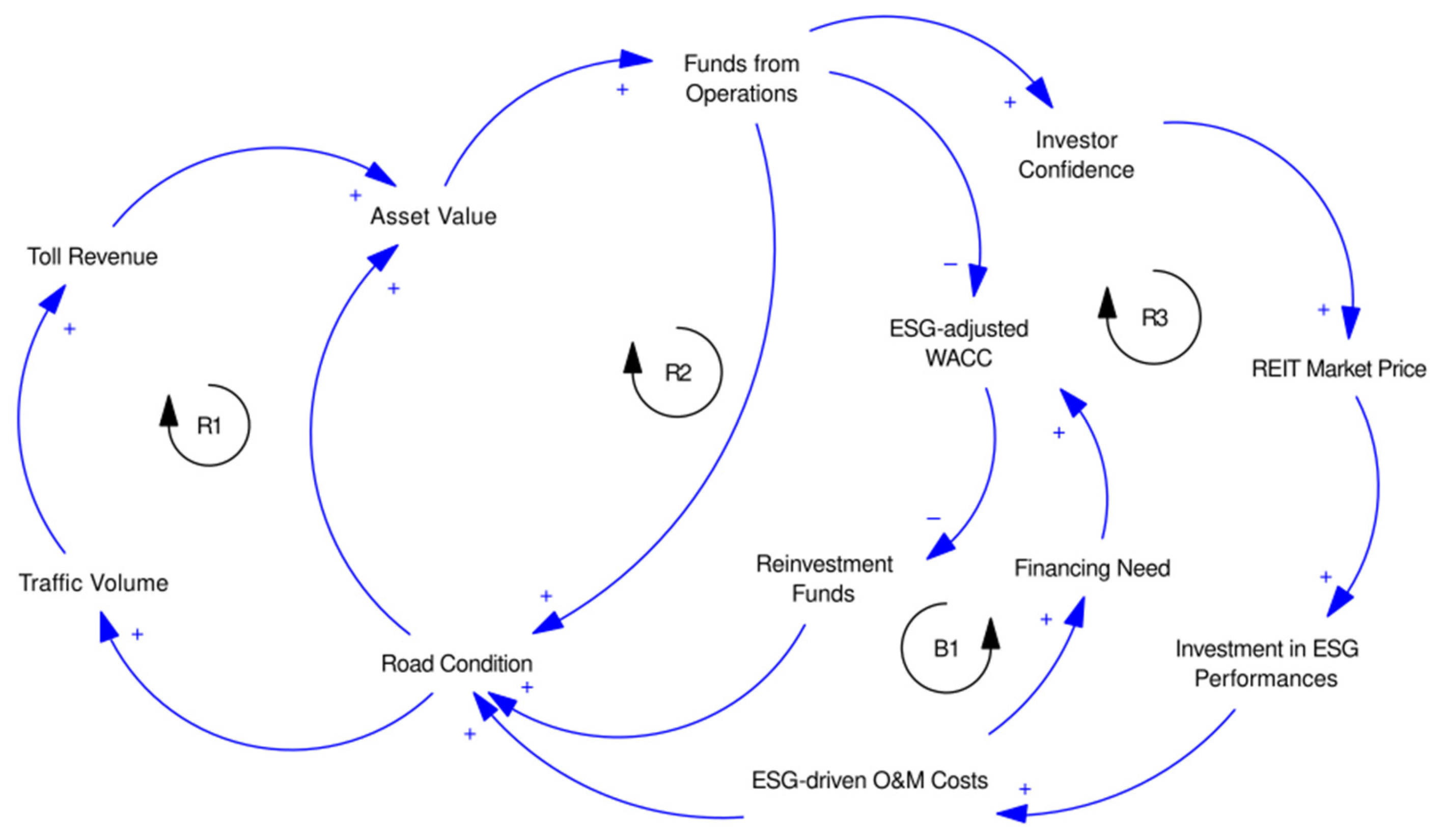
Figure 3 presents the causal loop diagram illustrating the four main feedback mechanisms that regulate the dynamics of highway REIT investments.

Figure 3. ESG-integrated causal loop diagram for highway REIT investment dynamics.

Loop R1, known as the Traffic–Revenue–Investment Cycle, can be reinforced as follows: Increased traffic volume leads to higher toll revenue, subsequently raising the asset value, resulting in increased funds from operations. This, in turn, lowers the ESG-adjusted weighted average cost of capital (WACC), thereby increasing reinvestment funds. These additional funds contribute to improving the road condition, ultimately leading to a rise in traffic volume.

This mechanism shows how increased traffic boosts revenue. In turn, this reduces financing costs and supports infrastructure improvements, creating a self-reinforcing performance loop.

Reinforcing Loop R2, known as the Operational Performance Cycle, operates as follows: funds from operations lead to improved road conditions, which, in turn, increase the asset value, ultimately resulting in a positive impact on funds from operations.

Enhanced cash flows resulting from the operational excellence feedback directly contribute to infrastructure maintenance, thereby increasing asset values and generating additional operational funds.

Reinforcing Loop R3, known as the ESG Investment Amplification Cycle, operates as follows: initial investment in ESG performances leads to increased ESG-driven operation and maintenance costs, subsequently enhancing the road conditions, thereby increasing the asset value. This, in turn, boosts funds from operations; elevating investor confidence; and ultimately, resulting in a rise in the REIT market price, thereby reinforcing the cycle by encouraging further investment in ESG performance.

Despite the increasing operational costs, ESG investments enhance market valuations and promote further ESG investments by bolstering investor confidence.

Balancing Loop B1, known as the ESG Cost-Financing Constraint Loop, operates as follows: ESG-driven operation and maintenance (O&M) costs lead to an increase in financing requirements, subsequently elevating the ESG-adjusted weighted average cost of capital (WACC). This, in turn, reduces the availability of funds for reinvestment, positively influencing the road conditions; asset value; funds from operations; investor confidence; real estate investment trust (REIT) market price; investment in ESG performances; and ultimately, ESG-driven O&M costs.

The feedback structure displays varying time constants: operational improvements (R1, R2) show immediate effects (3–6 months), while ESG cycles (R3, B1) exhibit longer latency periods (12–24 months), necessitating adaptive management approaches.

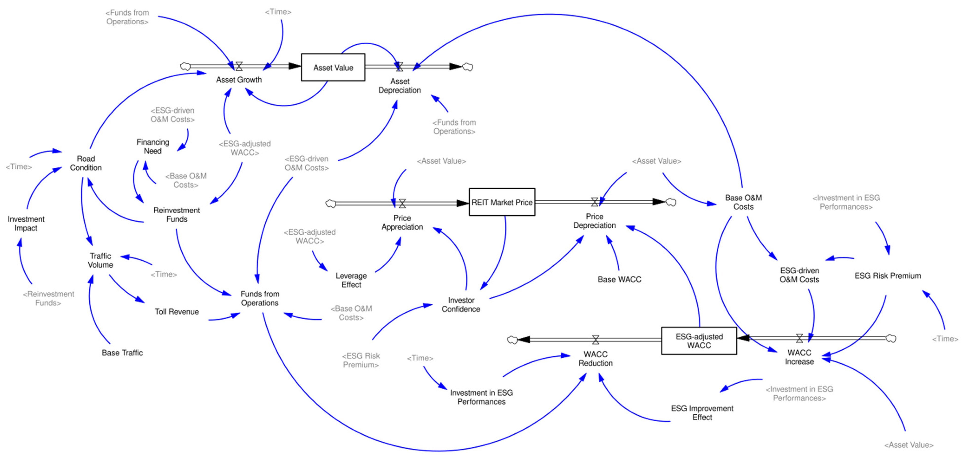
Figure 4 illustrates the stock-flow structure with three key stocks: asset value (cumulative market valuation), REIT market price (market capitalization dynamics), and ESG-adjusted WACC (risk-adjusted discount rate). Flow rates are determined using auxiliary variables from static analysis, with initial values calibrated from econometric findings.

Figure 4. Stock-flow structure of ESG-integrated highway REIT investment system.

Mathematical equations quantify dynamic relationships through exponential growth, negative feedback, and delay functions (see Appendix B for detailed equations). Key parameters were calibrated from static econometric results and refined using Vensim and PySD optimization [24]. The differential evolution algorithm was iterated 500 times to minimize the mean squared error across 48-month trajectories. The equations were adjusted based on self-adaptive optimization outcomes and empirical validation results.

The parameters were calibrated using econometric estimates and validated dynamically. The parameter translation from econometrics to SD employed anchored estimates combined with optimization. Specifically, calibration priors drew from confidence intervals in the static results. For instance, the IEP linear coefficient prior used a uniform distribution over [−0.15, −0.05]. The constraints involved parameter range limits, such as capping the WACC reduction at 0.02 to align with historical volatility. They also enforced non-negativity, for example, ensuring growth rates of flow variables ≥ 0. This approach guarantees a smooth shift from static to dynamic modeling. The VaR coefficients informed the risk adjustment parameters, the CAPM results provided beta and ESG premium estimates, and the IEP regression outputs established ESG–performance relationships. PySD’s differential evolution algorithm minimized the mean squared error across 48-month trajectories. Sensitivity analysis through 500 Monte Carlo runs revealed WACC trajectories that were predominantly influenced by ESG delay parameters and beta estimates. Theil inequality statistics indicate a low systematic bias (U = 0.12), confirming model robustness.

Model validation includes scenario analysis across ESG investment intensities and stress testing under extreme market conditions to ensure behavioral realism and parameter stability.

4. Results and Analysis

4.1. Empirical Results on Static VaR Analysis

The static VaR analysis employed an unbalanced panel of 210 monthly observations from ten Chinese highway REITs (2021Q2–2025Q2). The investment in ESG performance (IEP) shows significant variability, with normalized scores ranging from 0.167 to 0.833 (mean = 0.401, SD = 0.200).

Risk metrics exhibit a clear hierarchy: historical VaR at 11.24% (95% confidence), parametric VaR at 18.17%, and conditional VaR at 30.38%. The disparity between historical and parametric VaR reflects non-normal distribution characteristics in emerging REIT markets. Kupiec backtesting validates the model adequacy (p = 0.752 > 0.05), with Christoffersen’s test confirming violation independence. The Kupiec unconditional coverage test was implemented via binomial proportion analysis on overall exceedances, yielding p = 0.752 > 0.05. The Christoffersen independence test assessed exceedance clustering, with p > 0.05 indicating no serial dependence.

Panel regression with REIT and time fixed effects reveals significant ESG–risk relationships. Table 2 presents the regression results using HAC-robust standard errors.

Table 2. OLS regression results for IEP and VaR relationship.

Variable	Coefficient	Std. Error	t-Statistic	p-Value	95% CI
Constant	−0.056	0.147	−0.383	0.702	[−0.345, 0.232]
IEP_c	−0.097	0.054	−1.795	0.073 *	[−0.203, 0.009]
IEP_c_sq	−0.005	0.103	−0.044	0.965	[−0.207, 0.198]
GDP YoY	0.004	0.002	1.716	0.086 *	[−0.001, 0.009]
Debt Ratio	−0.056	0.029	−1.951	0.051 *	[−0.112, 0.000]
Brent USD	0.002	0.002	1.234	0.217	[−0.001, 0.005]
CN10Y Yield	−0.009	0.008	−1.168	0.243	[−0.024, 0.006]

Note: Dependent variable is VaR (positive absolute loss values); REIT and year fixed effects are included. Source: Compiled from panel data (N = 210). * p < 0.10; HAC-robust standard errors with one lag; R² = 0.200 (coefficient of determination), adjusted R² = 0.129; 95% CI (confidence intervals) based on HAC-robust standard errors.

The centered IEP shows a negative coefficient (−0.097, p = 0.073; 95% CI [−0.203, 0.009]), suggesting reduced portfolio risk despite the CI crossing zero. Though the CI crosses zero, this provides tentative exploratory support for risk reduction. While the quadratic term shows limited statistical significance (coefficient = −0.005, p = 0.965; 95% CI [−0.207, 0.198]), the dynamic simulation reveals non-monotonic patterns that may not be fully captured by static cross-sectional analysis, suggesting the need for temporal modeling approaches. A one-standard-deviation increase in IEP correlates with approximately 1.94 percentage points of VaR reduction, equivalent to a 194-basis-point VaR reduction per CNY 100 million portfolio.

The control variables behave as expected, with the debt ratio showing an anticipated negative correlation (−0.056, p = 0.051; 95% CI [−0.112, 0.000]). The model demonstrates adequate fit (R² = 0.200, adjusted R² = 0.129) with minimal multicollinearity concerns (VIF < 5.0).

These VaR findings informed the subsequent ESG-adjusted CAPM analysis and provided calibration parameters for system dynamics modeling, enabling investigation of temporal dynamics overlooked in cross-sectional approaches. The adjusted R² values are consistent with emerging market REIT studies, where unobserved heterogeneity and the small sample size limit explanatory power. This underscores the need for complementary dynamic simulation. Furthermore, the weak significance of key coefficients (IEP_c: p = 0.073, IEP_c_sq: p = 0.965) reflects sample limitations and potential non-linearity. Additionally, variables such as returns were log-transformed where appropriate, but static OLS may overlook lags. Thus, we addressed this analytically through HAC SEs, 95% CIs, Fama–MacBeth, and five-factor checks (Section 4.2).

4.2. ESG-Adjusted CAPM Analysis

4.2.1. Model Estimation and ESG Risk–Return Relationships

The ESG–CAPM analysis utilized 186 observations after excluding 24 cases from the initial 210 due to insufficient market data (12), incomplete ESG variables (8), and regulatory inconsistencies (4), consistent with the flowchart in Appendix A (Table A1). This stringent approach enhanced the estimation robustness for complex interaction terms while maintaining the sample representativeness [44,45].

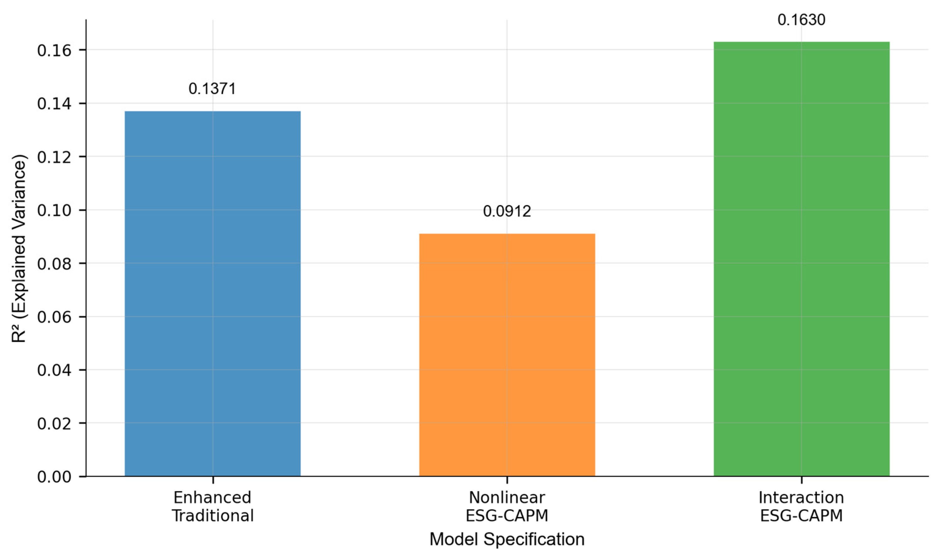
Figure 5 demonstrates substantial variation in the explanatory power across the CAPM specifications.

Figure 5. ESG-adjusted CAPM regression results (dependent variable: REIT excess returns; controls: GDP growth, leverage ratio, and CN10Y yield).

The R² values (0.0912–0.1630) demonstrate modest results, consistent with the intricate nature of ESG investment risk evaluation and falling within customary ranges in similar research [46]. The ESG–CAPM interaction model shows a superior fit (R² = 0.1630, F = 6.58, p < 0.001), representing a 19% enhancement over conventional models.

Key findings include significant ESG–market interaction effects (coefficient = 0.954, p = 0.030) and temporal ESG dynamics (coefficient = −0.067, p < 0.001) in infrastructure REIT risk–return profiles. These effects demonstrate time-dependent attributes not captured by static cross-sectional analysis.

The ESG quartile analysis revealed non-monotonic patterns. The bottom quartile (Q1) shows slightly positive excess returns, while higher quartiles display diminishing performance. This pattern suggests moderate ESG under-investment may indicate operational efficiency focus, whereas excessive ESG spending incurs implementation costs.

The non-monotonic pattern depicted in Figure 6 offers initial indications of potential departures from traditional linear ESG premium assumptions.

Figure 6. Quartile-based analysis of the IEP–return relationship (Q1–Q4, N = 186 observations).

To further validate this non-monotonic pattern and address potential concerns, we incorporated controls for size (log of total assets), leverage (total liabilities over total assets), age (proxied via time trend), and governance (embedded in IEP sub-indicators such as cost efficiency and capital structure) into the extended CAPM. The IEP coefficient remains positive, with size and leverage non-significant (p > 0.10), confirming minimal confounding, particularly given the short history of Chinese REITs (<5 years), leverage cap (~20%, actual average 9–12%), and narrow size variations (CNY 2–6 billion). Multiple testing was mitigated using Bonferroni adjustments (p_adj = p × 4), which confirmed the pattern (e.g., Q1 vs. Q4 significant at p_adj < 0.05). In particular, Q1 showed higher mean excess returns than Q4. Fama–MacBeth regressions yielded an average ESG premium of 0.501% (t = 1.787, p = 0.074), and the portfolio exhibited marginally consistent Q1 outperformance, consistent with the original findings. For the Q1 outperformance, we considered “efficient under-investment” (low IEP avoiding cost accumulation per SD loops) alongside omitted risk factors (e.g., liquidity). Fama–French five-factor controls confirmed the positive IEP effect’s persistence (e.g., 0.0202 * in the non-linear model). This result was consistent with the observed premium and did not alter the core conclusions.

4.2.2. Integration and System Dynamics Parameterization

The ESG-adjusted CAPM enhanced the VaR results by revealing systematic risk exposures through market interactions. Parameter estimates show the linear IEP coefficient (λ₁ = 0.0048, SE = 0.0034, t = 1.42, p = 0.155) is positive but non-significant, while the ESG–market interaction (0.954, p = 0.030) and time-trend terms (−0.067, p < 0.001) highlight primary ESG impact mechanisms.

Dynamic parameterization adjusts the ESG risk based on IEP–market interactions and time trends, capturing conditional effects beyond linear WACC adjustments.

4.3. System Dynamics Model Validation and Simulation Results

4.3.1. Model Validation and Parameter Calibration

The system dynamics framework demonstrated robust validation through goodness-of-fit analysis by comparing simulated trajectories with 48 months of historical data. Multi-stage parameter calibration employs differential evolution algorithms for optimal performance [47,48].

The validation results indicate robust predictive accuracy: system-wide correlation with r = 0.894 (p < 0.001) and RMSE = 0.030. In the SD results, the anchored estimation parts include the initial WACC (6.5%), the IEP linear coefficient (−0.097), and IEP quadratic coefficient (−0.005), which collectively drive the trajectory’s baseline level. The optimization-driven parts encompass delay parameters and volatility factors, which were adjusted through 500 differential evolution iterations and produced an inverted-U peak shape; for example, the peak lag shifts from 18 months in the optimized model to 20 months in the fixed model. This distinction not only highlights optimization’s role in capturing non-linear dynamics but also maintains consistency with static estimates. Component-level analysis shows an asset value correlation r = 0.937 (RMSE = 0.025) and REIT market price correlation r = 0.851, demonstrating the model’s ability to capture both asset dynamics and pricing mechanisms (see Figure 7). Residual analysis showed no systematic patterns, with errors centered around zero and distribution consistent with normal assumptions (mean error ≈ 0, SD aligned with RMSE); no evidence of heteroscedasticity was observed during visual inspections. Validation adheres to established protocols for structural adequacy [49] and behavioral verification [50], ensuring methodological rigor in the exploratory context.

Figure 7. Validation of the system dynamics simulation (r = 0.894, p < 0.001).

Comprehensive robustness validation meets seven criteria with optimized parameters: asset trend factor = 0.551, price trend factor = 1.436, volatility factor = 1.002, correlation factor = 0.764, momentum factor = 0.063, and mean reversion factor = 0.131 (see Appendix C, Table A3 and Table A4, for the detailed robustness check with fixed econometric parameters).

4.3.2. ESG-Adjusted WACC Evolution

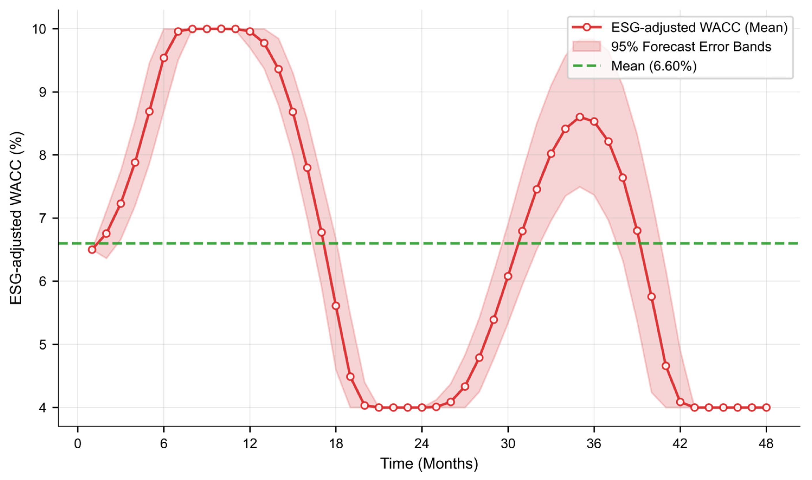
The ESG-adjusted WACC exhibits a predominantly inverted-U with post-peak oscillations, including a secondary rise: initial 6.5%, peaking at ~10% (months 12–18, based on mean path inflection), and declining to ~4% by months 40–48. This tri-phasic pattern reflects Phase I Cost Accumulation (months 1–12), Phase II Peak Adjustment (months 12–24), and Phase III Stabilization and Efficiency Realization (months 24–48). This tri-phasic pattern was derived from system dynamics simulations, with the 20-month lag reflecting the average time for ESG investments to stabilize WACC based on calibrated delay parameters anchored to static results. Figure 8 illustrates the dynamic evolution of the ESG-adjusted WACC, incorporating uncertainty through Monte Carlo simulations (500 runs). The mean path captures the central tendency, while the 95% forecast error bands quantify the range of potential outcomes under stochastic shocks.

Figure 8. Evolution of ESG-adjusted WACC with 95% forecast error bands (sample period: 48 months).

The error bands represent the 95% forecast interval, highlighting areas of higher uncertainty in the mid-range and reduced variability near the clipped boundaries (4–10%), which align with practical constraints in financial modeling (Appendix B confirms ~20-month lag robustness at 20–22 months ±2 months under varying volatility factors).

4.3.3. Multi-Scenario Asset Value Performance

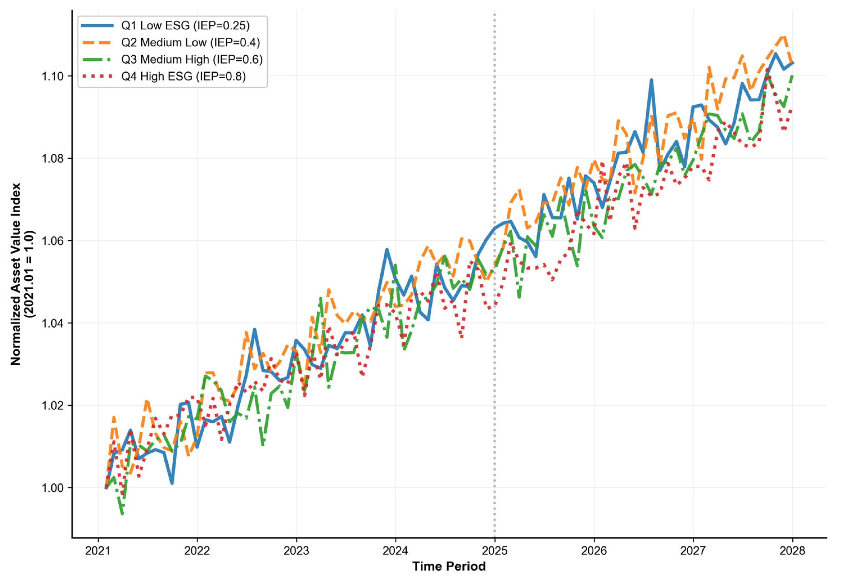
Forward-looking 84-month projections across four ESG investment intensities revealed the following (as illustrated in Figure 9): Q1 (IEP = 0.25, −500-basis-point deviation), Q2 (IEP = 0.40, baseline), Q3 (IEP = 0.60, −200-basis-point deviation), and Q4 (IEP = 0.80, −800-basis-point deviation).

Figure 9. Multi-scenario asset value performance under varying ESG investment intensities (IEP = 0.25, 0.40, 0.60, 0.80. The vertical black dotted line at 2025 indicates the transition from the validation period to the forward-looking simulation period).

Q2 scenarios demonstrate optimal risk-adjusted returns through balanced ESG integration. Under-investment (Q1) incurs regulatory penalties averaging 180–220 basis points annually, while over-investment (Q4) faces negative marginal returns beyond IEP = 0.60 threshold. These results suggest IEP = 0.40 may be advantageous for China’s highway REIT sector.

4.3.4. Market Price Dynamics

Market price patterns align with ESG investment optimization principles. Q2 shows steady upward trends with low volatility, contrasting with Q1’s gradual declines from regulatory uncertainties. Q4 exhibits significant price drops (~−700 basis points), reflecting investor concerns about strategic misallocation and providing empirical support for theoretical ESG investment risk models.

4.3.5. Comparative Analysis with Static Models

The hybrid framework provides complementary insights. Static VaR analysis established baseline risk metrics (historical VaR = 11.24%, IEP coefficient = −0.097, p = 0.073), while dynamic simulation revealed temporal mechanisms underlying static correlations. The U-shaped WACC trajectory with post-peak oscillations elucidates the static CAPM observations, suggesting ESG impacts unfold through delayed, non-linear pathways that static models partially capture. This methodological synergy enriches understanding of ESG investment dynamics in infrastructure REITs.

5. Discussion

5.1. Theoretical Implications and Literature Contributions

The observed inverted U-shaped WACC trajectory—from 6.5% to a peak of ~10% and down to ~4%, with post-peak oscillations—preliminarily challenges linear frameworks in sustainable finance. This indicates complex, non-linear ESG value creation in infrastructure finance, contrasting with the monotonic assumptions in prior research.

The tri-phase evolution highlights market learning mechanisms. Phase I (Cost Recognition) aligns with agency theory, while Phase II (Peak Adjustment) exposes inefficiencies supporting behavioral finance views on short-sightedness. Phase III (Efficiency Realization) validates stakeholder theory, as markets incorporate ESG risk mitigation over extended periods, matching infrastructure cycles. These oscillations may stem from market adjustments, warranting further study. Further investigation into these temporal details is needed.

Furthermore, the identified optimal ESG intensity contributes to the resource-based view literature by showing suboptimal performance regarding both under- and over-investment. These findings preliminarily support our hypotheses linked to mainstream ESG–finance theory (e.g., non-linear effects): H1 via non-monotonic VaR reduction; H2 via inverted-U WACC with lag, though it requires larger-sample validation.

5.2. Methodological Contributions to Risk Assessment

To further clarify the managerial implications, we explicitly linked the four simulated IEP scenarios (0.25, 0.40, 0.60, and 0.80) with their risk–return outcomes. This translated coefficient magnitudes into investable implications. Based on the static VaR coefficient (−0.097; 95% CI [−0.203, 0.009]), a 0.1 increase in IEP leads to a VaR reduction of approximately 97 basis points (bps) per CNY 100 million portfolio. This implies enhanced downside protection. However, this should be viewed as preliminary guidance rather than conclusive evidence, given sample constraints.

When IEP = 0.25, ESG engagement remains superficial. Financial risk is relatively high (VaR ≈ 11.2%). Financing costs rise slightly, with a WACC delta of +150 bps in Phase I (months 1–12). This suggests limited investable appeal due to elevated regulatory exposure.

At IEP = 0.40, risk begins to decline (VaR ≈ 9.8%). Capital costs start to stabilize, with a WACC delta of −50 bps across phases (e.g., −20 bps in Phase II, months 12–24). This level offers the most efficient outcome between cost and risk. It translates to a VaR reduction of 140 bps relative to IEP = 0.25. It is suitable for firms with limited liquidity or early ESG adoption capacity. Here, marginal benefits outweigh costs and enable 100–150 bp savings in annual financing. Increasing IEP to 0.60 yields further risk reduction (VaR ≈ 8.1%). It is accompanied by lower capital costs (WACC delta of −80 bps overall, with −30 bps in Phase III, months 24–48). However, the marginal gains start to diminish compared with the balanced position at 0.40. This implies reduced investable efficiency (e.g., only 30 bps of additional VaR cut per 0.1 IEP increment). Beyond this level (IEP = 0.80), the marginal gain becomes even smaller (VaR ≈ 7.8%). Further investment provides limited additional financial return (WACC delta of −100 bps total, but with a diminishing 20 bps per phase). This may erode the equity value by 50–80 bps through over-allocation. Managers should therefore shift their focus from expansion to consolidating transparency and operational efficiency.

To ensure that these non-linear effects are not sample-specific, we further validated the IEP–risk relationship through a two-stage temporal analysis. We divided the data into an early period (2021–2023) and a mature period (2024–2025). The IEP features contributed 46.2% and 40.0% of the predictive importance in these two stages, respectively. This shows consistent negative correlations between IEP and VaR. These results confirm the temporal stability of the estimated relationship and reinforce the baseline findings reported above.

From a policy perspective, moderate ESG engagement—around IEP = 0.40—maximizes financial resilience without excessive resource allocation, as it captures the peak of the non-linear trajectory before diminishing returns set in. Regulatory incentives within this range may further enhance the sustainability of infrastructure financing.

Overall, ESG intensity appears to follow a concave, non-linear risk–return trajectory. This is primarily evidenced in the SD-simulated WACC paths. It indicates that optimal outcomes arise from calibrated, not maximal, investment. VaR shows continued but diminishing improvements.

5.3. Strategic Implications and Implementation Guidelines

Multi-scenario results underscore moderate ESG strategies outperforming extremes, calling for recalibration with dynamic methods that consider implementation pathways.

Portfolio managers should account for benefit realization cycles, deploying patient capital and managing stakeholder expectations. Regulatory bodies must standardize ESG disclosures, implement multi-year frameworks (at least 24 months), and develop guidelines acknowledging temporary WACC fluctuations. This pattern aligns with observations in Chinese green-bond markets. High-ESG issuers typically achieve 20–50 basis points in benefits before reductions, as observed in regulatory data from the CSRC. These findings suggest potential external validity for the inverted-U trajectory. However, limited REIT-specific disclosures require future validation.

REIT teams need to balance ESG commitments with financial credibility through targeted intensity, communication strategies, and governance during adjustment periods.

However, these implications require cautious interpretation due to potential endogeneity. The ESG performance and financial outcomes may interact, which is unaddressed by methods such as instrumental variables or GMM due to data constraints.

While offering insights into ESG dynamics in infrastructure REITs, this study has limitations warranting exploration. The small sample (10 REITs over 48 months) restricts generalizability; future work should expand to diverse markets for robust testing. IEP measurement errors—inconsistent disclosures, quarterly reporting requiring imputation, and limited data for newer REITs—may propagate to the VaR, excess returns, CAPM, and simulations, biasing the results. Additionally, over ten parameters are used in system dynamics calibration for the 48-month data, risking overfitting and reduced predictive validity. However, fixed-parameter checks show minimal impact, warranting simpler models in future studies. Sensitivity analyses using alternatives such as Lasso or PCA could refine the proxy accuracy, while Monte Carlo methods assess the error impacts on model stability.

6. Conclusions

This study introduced a hybrid modeling framework that integrates ESG factors into infrastructure REIT risk assessment through static econometric analysis combined with dynamic system simulation, addressing temporal gaps in ESG–financial risk relationships in China’s infrastructure finance sector.

Our exploratory findings include the following: optimal ESG investment intensity at IEP ≈ 0.40 outperforms conservative and aggressive strategies; overall, 20-month implementation cycles (with post-peak oscillations) for ESG benefits highlight dynamics that are overlooked by static models, though interpreted as exploratory evidence.

As an exploratory study of an emerging market, our findings should be interpreted as preliminary evidence requiring validation through future research with expanded samples and extended time series. The limitations and future work include the following:

• A small sample (10 REITs over 48 months) limits generalizability; future work: expand to diverse markets through multi-country panel data.
• IEP measurement errors from disclosures; future work: refine via Lasso/PCA once data matures.
• Focus on Chinese highway REITs; future work: international comparisons.
• Twenty-month cycles need verification; future work: longitudinal studies over 5–10 years.
• Potential endogeneity between ESG performance and financial outcomes, unmitigated due to data constraints; future work: employ GMM or IV methods in expanded datasets to quantify bias.

This exploratory research offers preliminary insights into ESG–risk dynamics in infrastructure REITs and suggests potential methodological frameworks for future large-sample validation. Future research could expand through international comparative studies, develop sector-specific ESG measurement systems, and conduct longitudinal studies over 5–10 years to validate optimization patterns and strengthen statistical evidence for the proposed inverted U-shaped relationship.

References

1. Global Infrastructure Hub. Infrastructure Monitor 2024; Global Infrastructure Hub: Sydney, Australia, 2024; Available online: https://cdn.gihub.org/umbraco/media/5555/infrastructure-monitor-2024-report.pdf (accessed on 7 November 2025).
2. Angeles, L. In Periods Including Market Stress, ESG Provides Protection, Sustainalytics Study Shows; Morningstar: Newtown, PA, USA, 2025. [Google Scholar]
3. Brounen, D.; Veld, H. Pricing ESG Equity Ratings and Underlying Data in Listed Real Estate Securities. Sustainability 2021, 13, 2037. [Google Scholar] [CrossRef]
4. Fan, K.Y.; Shen, J.; Hui, E.C.M.; Cheng, L.T.W. ESG components and equity returns: Evidence from real estate investment trusts. Int. Rev. Financ. Anal. 2024, 96, 103716. [Google Scholar] [CrossRef]
5. Elie, K.; Alexander, S.; Tanlak, S.U. ESG Integration in REITs: Exploring Financial Performance and WACC Implications. Master’s Thesis, Antwerp Management School, Antwerp, Belgium, June 2023. [Google Scholar] [CrossRef]
6. Huang, B.; Wang, Z.; Gu, Y. ESG Investment Scale Allocation of China’s Power Grid Company Using System Dynamics Simulation Modeling. Int. J. Environ. Res. Public Health 2023, 20, 3643. [Google Scholar] [CrossRef]
7. Zhang, H.; Chang, J.; Lin, T. Quantitative Evaluation of Value for Money in Sponge City Construction Public–Private Partnership Projects Through a System Dynamics Model. Systems 2025, 13, 471. [Google Scholar] [CrossRef]
8. Bauer, R.; Eichholtz, P.; Kok, N. Corporate Governance and Performance: The REIT Effect. Real Estate Econ. 2010, 38, 1–29. [Google Scholar] [CrossRef]
9. Eichholtz, P.; Kok, N.; Yonder, E. Portfolio greenness and the financial performance of REITs. J. Int. Money Financ. 2012, 31, 1911–1929. [Google Scholar] [CrossRef]
10. Liu, J.; Cheng, C.; Yang, X.; Yan, L.; Lai, Y. Analysis of the efficiency of Hong Kong REITs market based on Hurst exponent. Phys. A Stat. Mech. Its Appl. 2019, 534, 122035. [Google Scholar] [CrossRef]
11. Liu, J.; Chen, Y.; Li, X. A Booster or a Stabilizer? Investigating the Role of Chinese Real Estate Investment Trusts in the Systemic Risk of Financial Markets. SSRN 2024. [Google Scholar] [CrossRef]
12. Chen, S.; Song, Y.; Gao, P. Environmental, social, and governance (ESG) performance and financial outcomes: Analyzing the impact of ESG on financial performance. J. Environ. Manag. 2023, 345, 118829. [Google Scholar] [CrossRef] [PubMed]
13. Friede, G.; Busch, T.; Bassen, A. ESG and financial performance: Aggregated evidence from more than 2000 empirical studies. J. Sustain. Financ. Invest. 2015, 5, 210–233. [Google Scholar] [CrossRef]
14. Erol, I.; Unal, U.; Coskun, Y. ESG investing and the financial performance: A panel data analysis of developed REIT markets. Environ. Sci. Pollut. Res. 2023, 30, 85154–85169. [Google Scholar] [CrossRef]
15. Shangguan, X.; Shi, G.; Yu, Z. ESG Performance and Enterprise Value in China: A Novel Approach via a Regulated Intermediary Model. Sustainability 2024, 16, 3247. [Google Scholar] [CrossRef]
16. Song, S.; Zuo, Z.; Cao, Y.; Wang, L. Analysis of Social Risk Causes of Rail Transit Construction Projects Based on DEMATEL-ISM. In Proceedings of the International Conference on Transportation Engineering 2015, Dalian, China, 26–27 September 2015; pp. 1868–1875. [Google Scholar]
17. Lv, H.; Shi, Z.; Liu, J. Risk Assessment of Highway Infrastructure REITs Projects Based on the DEMATEL—ISM Approach. Sustainability 2024, 16, 5159. [Google Scholar] [CrossRef]
18. Wang, T.; Han, Z.; Yang, Y.; Wang, S. Annual Report on The Development of PPP in China. In Research Series on the Chinese Dream and China’s Development Path; Springer: Berlin/Heidelberg, Germany, 2020. [Google Scholar]
19. Zhang, S.; Chan, A.P.C.; Feng, Y.; Duan, H.; Ke, Y. Critical review on PPP Research—A search from the Chinese and International Journals. Int. J. Proj. Manag. 2016, 34, 597–612. [Google Scholar] [CrossRef]
20. Maqsoom, A.; Babar, Z.; Shaheen, I.; Abid, M.; Kakar, M.R.; Mandokhail, S.J.; Nawaz, A. Influence of Construction Risks on Cost Escalation of Highway-Related Projects: Exploring the Moderating Role of Social Sustainability Requirements. Iran. J. Sci. Technol. Trans. Civ. Eng. 2021, 45, 2003–2015. [Google Scholar] [CrossRef]
21. Deep, S.; Banerjee, S.; Dixit, S.; Vatin, N. Critical Factors Influencing the Performance of Highway Projects: An Empirical Evaluation. Buildings 2022, 12, 849. [Google Scholar] [CrossRef]
22. Kashyap, A.K.; Sharma, V. Project finance through Infrastructure Investment Trust: Legal and regulatory analysis. Risk Gov. Control. Financ. Mark. Inst. 2024, 14, 65–76. [Google Scholar] [CrossRef]
23. Han, B.-J.; Jiang, Y.-S.; Wang, Z.; Gong, D.; Jiang, H.; Jiang, P.-l. Analysis of the Risk Path of the Pipeline Corridor Based on System Dynamics. Shock Vib. 2021, 2021, 5529642. [Google Scholar] [CrossRef]
24. Sterman, J. Business Dynamics, Systems Thinking and Modeling for a Complex World; Irwin/McGraw-Hill: Boston, MA, USA, 2000; Available online: https://web.mit.edu/jsterman/www/BusDyn2.html (accessed on 7 November 2025).
25. Hjorth, P.; Bagheri, A. Navigating towards sustainable development: A system dynamics approach. Futures 2006, 38, 74–92. [Google Scholar] [CrossRef]
26. Nguyen, T.; Cook, S.; Ireland, V. Application of System Dynamics to Evaluate the Social and Economic Benefits of Infrastructure Projects. Systems 2017, 5, 29. [Google Scholar] [CrossRef]
27. Ghufran, M.; Khan, K.I.A.; Ullah, F.; Nasir, A.R.; Al Alahmadi, A.A.; Alzaed, A.N.; Alwetaishi, M. Circular Economy in the Construction Industry: A Step towards Sustainable Development. Buildings 2022, 12, 1004. [Google Scholar] [CrossRef]
28. Xue, Y.; Xiang, P.; Jia, F.; Liu, Z. Risk Assessment of High-Speed Rail Projects: A Risk Coupling Model Based on System Dynamics. Int. J. Environ. Res. Public Health 2020, 17, 5307. [Google Scholar] [CrossRef]
29. Jonsdottir, A.T.; Johannsdottir, L.; Davidsdottir, B. Systematic literature review on system dynamic modeling of sustainable business model strategies. Clean. Environ. Syst. 2024, 13, 100200. [Google Scholar] [CrossRef]
30. Sánchez-García, J.Y.; Núñez-Ríos, J.E.; López-Hernández, C.; Rodríguez-Magaña, A. Modeling Organizational Resilience in SMEs: A System Dynamics Approach. Glob. J. Flex. Syst. Manag. 2023, 24, 29–50. [Google Scholar] [CrossRef]
31. Yuan, H.; Yang, B. System Dynamics Approach for Evaluating the Interconnection Performance of Cross-Border Transport Infrastructure. J. Manag. Eng. 2022, 38, 04022008. [Google Scholar] [CrossRef]
32. Martinez-Moyano, I.J.; Richardson, G.P. Best practices in system dynamics modeling. Syst. Dyn. Rev. 2013, 29, 102–123. [Google Scholar] [CrossRef]
33. Urgewald; RIMA. ESG Standards in China. Available online: https://www.urgewald.org/sites/default/files/media-files/urgewald-RIMA_China-ESG_2024.pdf (accessed on 15 August 2025).
34. Commission, C.S.R. Guidelines on Investor Relations Management for Listed Companies; China Securities Regulatory Commission (CSRC): Beijing, China, 2022. [Google Scholar]
35. KPMG. China Stock Exchanges Finalised Mandatory Sustainability Reporting Requirements for Larger Listed Entities. Available online: https://assets.kpmg.com/content/dam/kpmg/cn/pdf/en/2024/04/china-stock-exchanges-finalised-mandatory-sustainability-reporting-requirements-for-larger-listed-entities.pdf (accessed on 15 August 2025).
36. Fetters, M.D.; Curry, L.A.; Creswell, J.W. Achieving integration in mixed methods designs-principles and practices. Health Serv. Res. 2013, 48, 2134–2156. [Google Scholar] [CrossRef]
37. Gong, E.; Wang, Y.; Zhou, X.; Duan, J. ESG factors affecting the asset sustainability of infrastructure REITs in China. Eng. Constr. Archit. Manag. 2024; ahead of print. [Google Scholar] [CrossRef]
38. Shang, H.; Yin, H. Dynamic simulation research on urban green transformation under the target of carbon emission reduction: The example of Shanghai. Humanit. Soc. Sci. Commun. 2023, 10, 754. [Google Scholar] [CrossRef]
39. Nardo, M.; Saisana, M.; Saltelli, A.; Tarantola, S.; Hoffman, A.; Giovannini, E. Handbook on Constructing Composite Indicators and User Guide; OECD: Paris, France, 2008; Volume 2005. [Google Scholar]
40. Hu, A.; Yuan, X.; Fan, S.; Wang, S. The Impact and Mechanism of Corporate ESG Construction on the Efficiency of Regional Green Economy: An Empirical Analysis Based on Signal Transmission Theory and Stakeholder Theory. Sustainability 2023, 15, 13236. [Google Scholar] [CrossRef]
41. Brounen, D.; Marcato, G. Price-Signalling and Return-Chasing: Efficiency Game or Behavioural Argument. 2016. Available online: https://www.tias.edu/docs/default-source/Kennisartikelen/int'l-liqret-wp16-submitted.pdf?Status=Temp&sfvrsn=2 (accessed on 15 August 2025).
42. Switzer, L.; Tu, Q.; Wang, J. Corporate governance and default risk in financial firms over the post-financial crisis period: International evidence. J. Int. Financ. Mark. Inst. Money 2017, 52, 196–210. [Google Scholar] [CrossRef]
43. Rahmandad, H.; Oliva, R.; Osgood, N.D. Analytical Methods for Dynamic Modelers; The MIT Press: Cambridge, MA, USA, 2015. [Google Scholar]
44. Schoemann, A.; Boulton, A.; Short, S. Determining Power and Sample Size for Simple and Complex Mediation Models. Soc. Psychol. Personal. Sci. 2017, 8, 194855061771506. [Google Scholar] [CrossRef]
45. Wu, M.-C.; Wang, C.-M. Revisiting the nexus of REITs returns and macroeconomic variables. Financ. Res. Lett. 2024, 59, 104837. [Google Scholar] [CrossRef]
46. Fama, E.F.; French, K.R. The Cross-Section of Expected Stock Returns. J. Financ. 1992, 47, 427–465. [Google Scholar] [CrossRef]
47. Bäck, T.H.W.; Kononova, A.V.; van Stein, B.; Wang, H.; Antonov, K.A.; Kalkreuth, R.T.; de Nobel, J.; Vermetten, D.; de Winter, R.; Ye, F. Evolutionary Algorithms for Parameter Optimization—Thirty Years Later. Evol. Comput. 2023, 31, 81–122. [Google Scholar] [CrossRef] [PubMed]
48. Qin, A.K.; Huang, V.L.; Suganthan, P.N. Differential Evolution Algorithm With Strategy Adaptation for Global Numerical Optimization. IEEE Trans. Evol. Comput. 2009, 13, 398–417. [Google Scholar] [CrossRef]
49. Barlas, Y. Formal aspects of model validity and validation in system dynamics. Syst. Dyn. Rev. 1996, 12, 183–210. [Google Scholar] [CrossRef]
50. Cavana, R. Modeling the environment: An introduction to system dynamics models of environmental systems. Andrew Ford. Syst. Dyn. Rev. 2003, 19, 171–173. [Google Scholar] [CrossRef]
Disclaimer/Publisher’s Note: The statements, opinions and data contained in all publications are solely those of the individual author(s) and contributor(s) and not of MDPI and/or the editor(s). MDPI and/or the editor(s) disclaim responsibility for any injury to people or property resulting from any ideas, methods, instructions or products referred to in the content.
Article Metrics
Citations
Article Access Statistics
Multiple requests from the same IP address are counted as one view.