Research on Traffic Accident Severity Level Prediction Model Based on Improved Machine Learning

Abstract

Traffic accidents occur frequently, causing significant losses to people’s lives and property safety. Accurately predicting the severity level of traffic accidents is of great significance. Based on traffic accident data, this study comprehensively considers various influencing factors such as the geographical location, road conditions, and environment. The data are divided into accident-related categories, weather-related categories, and road- and environment-related categories. The machine learning method is improved through integration for the accident level prediction. In the experiment, effective preprocessing measures were taken for problems such as data imbalance, missing values, the encoding of categorical variables, and the standardization of numerical features. The unbalanced distribution of “Severity” was improved through under-sampling and over-sampling techniques. Firstly, we adopted a multi-stage fusion strategy. A multi-layer perceptron (MLP) was used for the preliminary prediction, and then its result was combined with the original features to form a new feature. Decision tree, XGBoost, and random forest algorithms, respectively, were applied for the secondary prediction. The analysis results show that the improved machine learning model is significantly superior to a single model in the overall performance. The “MLP + random forest” model performs well in evaluation indicators such as the accuracy, recall rate, and F1 value. The accuracy rate is as high as 94%. In the prediction of different traffic accident severity levels (minor, moderate, and severe), the improved machine learning model also generally shows better performance and stability. The research results of this study have broad prospects in the field of intelligent driving. It can realize real-time accident prediction and early warnings, and provide decision support for drivers and autonomous driving systems. The research also provides a scientific basis for traffic planning and management departments to improve driving conditions and reduce the probability and losses of traffic accidents.

1. Introduction

Traffic accidents are unexpected and the worst situations for road users, yet they occur frequently [1]. Regrettably, in the past few years, with the explosive increase in car ownership, the number of traffic accidents has been on the rise. This has caused significant losses to people’s lives and property safety. According to relevant data, many people die in traffic accidents every year in various countries. Taking the United States, a country on wheels, as an example, in 2023, 40,990 people died in car accidents across the United States. The number of fatalities in 15 states increased. For instance, compared to the previous year, the traffic fatality rate in Washington State increased by nearly 11%, and, in Idaho, it increased by nearly 29% [2]. In China, a country with a growing number of cars, there were 10 million traffic accidents in 2023, with the number of deaths reaching 100,000 and the number of injured reaching 2 million [3]. According to relevant research, the occurrence of car accidents and their severity levels (mild, moderate, and severe) are significantly affected by factors such as the geographical location, road conditions, and environment where vehicles are traveling [4,5]. Therefore, predicting the severity level of traffic accidents based on different geographical locations, road conditions, and environmental factors has important practical significance. For example, the prediction of traffic accidents and their severity levels can provide decision support for drivers and autonomous driving systems, and also provide a scientific basis for traffic planning and management departments to improve driving conditions and reduce the probability and losses of traffic accidents [1].

In recent years, machine learning technology has developed rapidly. In the field of machine learning, continuously optimized algorithms can process large-scale data and extract more valuable information [6,7,8]. Multiple machine learning algorithms can be combined through an integrated mode to further improve the adaptability and stability of the model [9,10,11,12,13,14]. Machine learning technology is widely used in many accident prediction fields. In the field of construction safety, some scholars identify potential risk factors and issue early warnings by analyzing a large amount of historical data. However, in the transportation field, various advanced statistical models have also been proposed. These models offer different perspectives for crash severity prediction and show promise in capturing the complexity of crash data [15,16].

There has been a large number of relevant studies on machine learning in various engineering fields. Nayan used machine learning to bypass the seismic analysis of buildings and perform the damage estimation of reinforced concrete buildings [17]. Li proposed a hybrid method based on traditional multiphase flow mechanisms and machine learning models to determine the safe operational MTB for multiphase pipeline transportation processes [18]. In the field of industrial production, some scholars have also used machine learning algorithms such as LSTM networks and the SVM to monitor the operating status of equipment and predict failures in order to avoid safety accidents [9,10,11,12,13,14]. In fields like healthcare, environment, and geology, machine learning has also showed great potential [19,20,21,22,23]. When it comes to traffic accident prediction, there were also studies that employed different machine learning models for it [24,25,26,27]. Some studies were dedicated to developing innovative models and enhancing the prediction accuracy of models by improving the original machine learning algorithms. For example, Chen introduced the CTM to simulate traffic data and combined it with physical data to develop a collision prediction model to improve the collision prediction ability [28]. Pérez-Sala proposed a deep learning model based on convolutional neural networks and genetic algorithms to predict the severity level of traffic accidents [29]. Berhanu introduced an innovative approach that integrated random forest (RF) models, collision rates, and spatial network analysis to reduce road traffic accidents (RTAs) and congestion, and to provide drivers with safe route recommendations [25]. Meanwhile, data preprocessing and analysis were crucial in traffic accident research and could solve problems such as sample imbalance. Some scholars have attempted to combine data preprocessing, feature extraction, sampling processing, and other methods to improve the accuracy of traffic accident prediction. For instance, Pourroostaei analyzed the characteristics of traffic accident data by using a preprocessing model combined with machine learning technology [6]. Labib tried to improve the accuracy through dataset preprocessing and feature selection when using machine learning to analyze and predict road traffic accidents [7]. De combined latent class clustering and Bayesian networks to analyze the characteristics of traffic accident data [8]. Additionally, some scholars also analyzed the impact of the comprehensive application of sampling techniques on the preprocessing effect of historical traffic accident data [30,31,32,33]. However, currently, machine learning still faces challenges such as low model accuracy and insufficient data preprocessing in accident prediction modeling. Among them, Ali pointed out that the universality and accuracy of some models needed to be verified [34]. When Infante used logistic regression and multiple machine learning models to classify and evaluate the severity level of road traffic accidents, he found that some models were not effective in accident classification [27]. Depaire applied latent class clustering to traffic accident analysis and pointed out that the model might obtain a local rather than a global optimal solution [35]. De pointed out that traffic accident prediction currently faces challenges such as difficult data integration and difficult asynchronous data [36].

Therefore, in this study, by optimizing and integrating multiple machine learning methods, an improved machine learning model is constructed and is combined with multiple data preprocessing methods, such as under-sampling and over-sampling, to predict the severity level of traffic accidents. Based on the road accident data from 15 January 2016 to 1 January 2022 in the United States [4,5], this study divides the data into accident-related categories, weather-related categories, and road- and environment-related categories, covering many variables such as the Distance (mi), Side, State, Timezone, Temperature (F), etc. It not only takes into account the direct features related to accidents but also integrates the data from multiple dimensions, such as weather conditions and road environments. Through the integration of these multi-source features, the model can capture the factors influencing the severity of accidents in a more comprehensive manner. First, under-sampling and over-sampling are performed on the sample data to solve the problem of sample imbalance. Secondly, preprocessing operations, such as encoding relevant variables and the handling of missing values, are performed. Thirdly, through constructing a multi-layer perceptron model (MLP), preliminary prediction is carried out. The prediction result is taken as a new feature and integrated into the source data, and then brought into decision tree, XGBoost, and random forest algorithms for secondary prediction. The results show that this improved machine learning model shows significant advantages in the applicability and accuracy of the traffic accident level prediction. Meanwhile, as verified by experiments, this method enhances the model’s ability to understand and classify data, and it also has a good stability and generalization ability against external data interference.

2. Experimental Principles and Methods

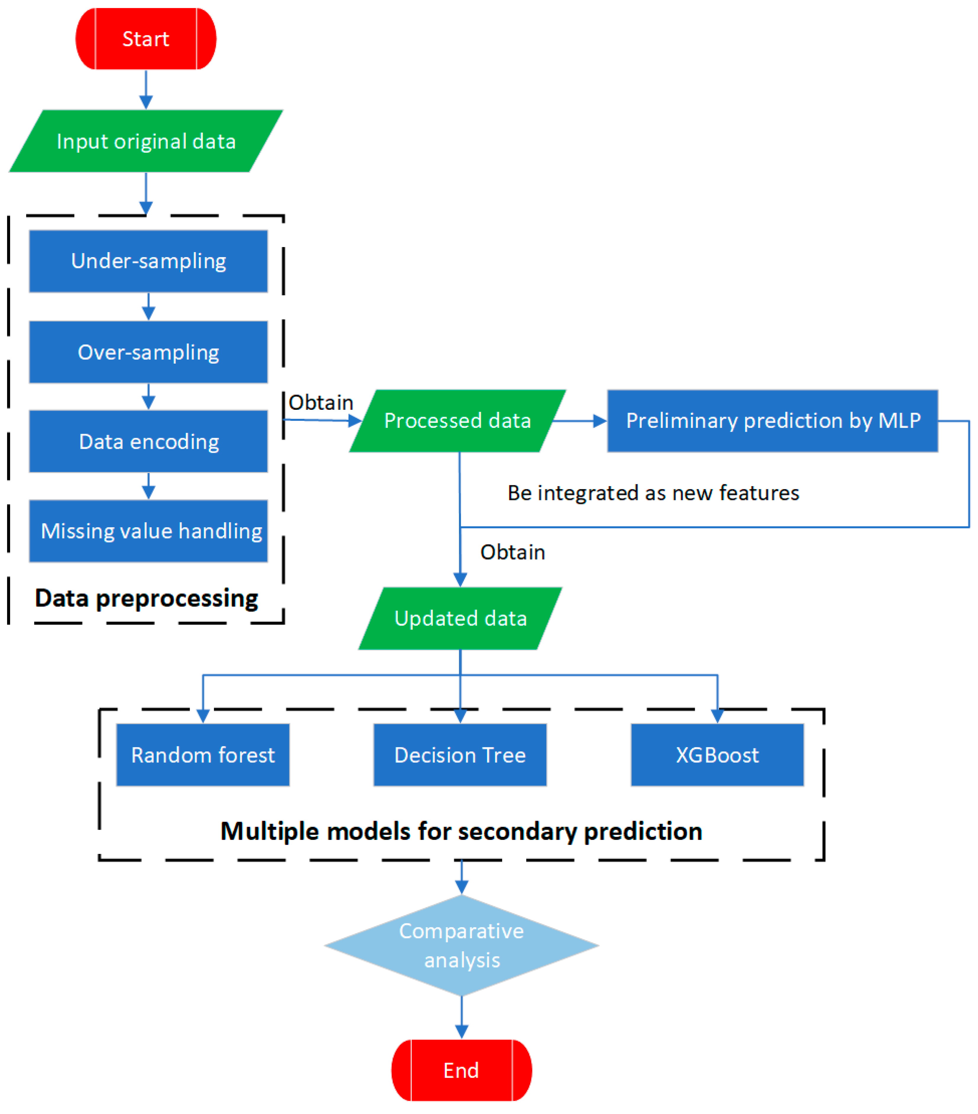
This study first performs under-sampling and over-sampling on historical traffic accident data to solve the common problem of sample imbalance. Then, an MLP is used for the preliminary classification prediction of accident severity levels, and decision tree, XGBoost, and random forest algorithms, respectively, are used for the secondary classification prediction of the data. The specific process is shown in Figure 1.

Since the samples of traffic accident data are often highly imbalanced, traditional models usually have a poor recognition ability for minority class samples and are prone to overfitting for majority class samples. To precisely address this issue, in this study, under-sampling is performed on the majority class of mild accident samples, while over-sampling is applied to the minority class of moderate and severe samples. This ensures a more balanced distribution of accident samples with different severity levels and enables more accurate predictions.

Firstly, the multi-layer perceptron (MLP) is used for the preliminary prediction of the accident severity. Its multi-layer structure and activation functions can explore the deep feature relationships. The output results are integrated into the source data as new features. In this way, the source data incorporate the potential feature patterns learned by the MLP. The hidden associations of accident features in the high-dimensional space are revealed by the MLP and integrated into the data, injecting strong feature information for the secondary prediction of the subsequent models, and improving the discriminative ability and prediction accuracy of the model for the accident severity from multiple dimensions.

2.1. Sampling Technique and Data Preprocessing

In a dataset, when the number of samples in a certain category is much larger than that in other categories, there is a situation of data imbalance [32]. Under-sampling is to randomly select a part of samples from the majority class samples to achieve a relatively balanced state with the number of minority class samples [31]. The principle is to reduce the dominant position of the majority class in model training by reducing the number of majority class samples, so that the model can pay equal attention to the characteristics and patterns of samples of various categories, avoid overfitting of the majority class samples by the model, and improve the recognition ability for the minority class. Over-sampling operates on minority class samples. By increasing the number of minority class samples in a way with or without replacement, the purpose of achieving a relatively balanced number with the majority class samples is achieved [33]. The principle of over-sampling is to increase the number of minority class samples so that the model has more opportunities to learn the characteristics of the minority class, thereby improving the sensitivity and recognition ability of the model for the minority class.

Historical traffic accident data often have the problem that the data with low accident severity levels account for a large proportion, while the data with high accident levels account for a relatively small proportion. Therefore, under the premise that the absolute sample size of different accident level data meets the preprocessing requirements, this study reasonably adjusts the gap in the relative sample size through under-sampling and over-sampling to solve the common problem of sample imbalance in historical traffic accident data. Meanwhile, preprocessing operations such as data encoding and standardization are also helpful in dealing with data imbalance. Categorical variables in the data (such as “Side”, “Weather_Condition”, etc.) need to be encoded into numerical forms so that the model can handle them better. In traffic accident data, categorical variables have an important impact on the accident severity. Taking “Weather_Condition” as an example, its different values (such as “Fair”, “Cloudy”, etc.) have complex associations with the accident severity. After encoding these categories into numerical values, the model can process them mathematically and better learn the relationship patterns between different weather conditions and the accident severity. Especially in the case of data imbalance, encoding helps the model to more accurately distinguish the feature differences in the different severity levels of accidents.

2.2. MLP

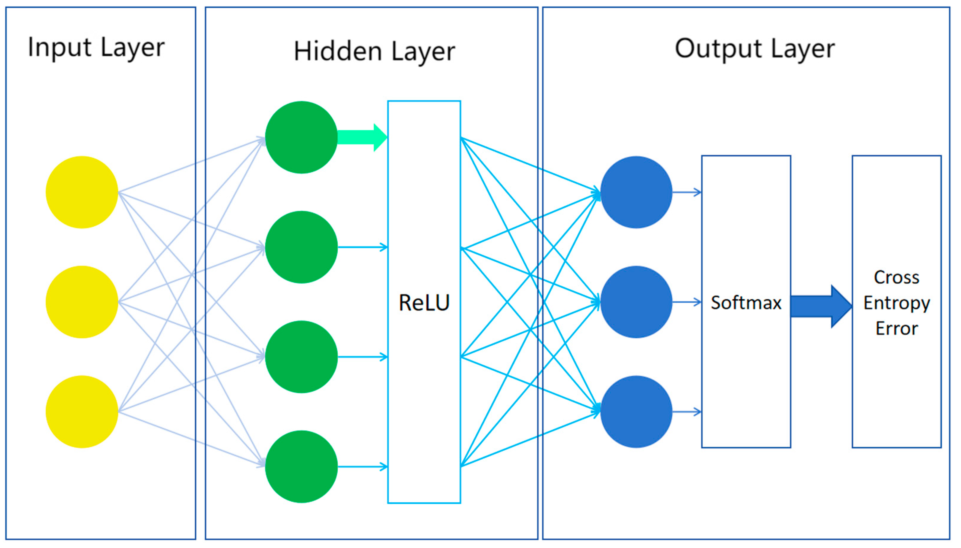
The MLP is an artificial neural network model composed of multiple neuron layers, including the input layer, hidden layer, and output layer [37]. The structure of the MLP is shown in Figure 2. The input layer receives the input data. The hidden layer learns the feature representations, and the output layer produces the final prediction result. Each neuron in the hidden layer and the output layer has an activation function for introducing nonlinear mapping.

The basic component unit of the MLP is a neuron. Each neuron receives input signals from neurons in the previous layer. These input signals are weighted and summed, and a bias term is added to obtain a total input value, as shown in calculation Formula (1):

$$z={\displaystyle \sum _i{{\displaystyle w}}_i{{\displaystyle x}}_i}+b$$

(1)

where $z$ is the total input value, ${\mathrm{w}}_{\mathrm{i}}$ is the weight connecting the $\mathrm{i}$-th neuron in the previous layer, ${\mathrm{x}}_{\mathrm{i}}$ is the output value of the $\mathrm{i}$-th neuron in the previous layer, and $b$ is the bias.

Then, this total input value is nonlinearly transformed through an activation function to obtain the output value of this neuron. In this experiment, the ReLU function is used for the activation, as shown in calculation Formula (2):

$$f(z)=\max (0,z)$$

(2)

The output layer uses the softmax activation function to convert the model’s output into the probability distribution of each category to meet the needs of multi-classification tasks. By reasonably configuring the number of neurons and activation functions in each layer, the model can learn the potential patterns and regularities in the data. The output probability distribution is shown in calculation Formula (3):

$$softmax\left(\left[z_4^1,z_4^2,z_4^3\right]\right)=\left[{\displaystyle \frac{e^{z_4^1}}{e^{z_4^1}+e^{z_4^2}+e^{z_4^3}}},{\displaystyle \frac{e^{z_4^2}}{e^{z_4^1}+e^{z_4^2}+e^{z_4^3}}},{\displaystyle \frac{e^{z_4^3}}{e^{z_4^1}+e^{z_4^2}+e^{z_4^3}}}\right]$$

(3)

During the training process, a loss function is defined to measure the difference between the probability distribution predicted by the model and the real label $y$. The Adam optimizer is used to update the weights and biases of the model with a learning rate of 0.001 to minimize the loss function, as shown in calculation Formula (4):

$$loss=-{\displaystyle \sum _i{{\displaystyle y}}_i\log ({{\displaystyle \widehat{y}}}_i)}$$

(4)

During the training process, this study conducts 100 rounds of training. Each round processes the data of 32 samples. Through continuous iteration and optimization, the MLP model can learn the complex relationship between the input data and “Severity”, thereby realizing the preliminary prediction and classification of the severity level of traffic accidents. Next, this study takes the result predicted by the MLP as a new feature and combines the original features to use algorithms such as the decision tree, XGBoost, and random forest, respectively, for the secondary prediction so to explore the classification effect.

2.3. Decision Tree

The decision tree is a machine learning algorithm that makes decisions based on a tree structure. It constructs decision rules by recursively dividing features to achieve the prediction of target variables [38]. In this study, the decision tree algorithm is used to perform the secondary prediction on the data preliminarily processed by the MLP. By adjusting parameters such as the depth and splitting criteria of the decision tree, the performance of the model is optimized. The schematic diagram of the decision tree process is shown in Figure 3.

The decision tree constructs decision rules by recursively dividing the data. Its basic principle is to select the optimal feature and splitting point based on criteria such as the information gain and the Gini index. Suppose the dataset is $D$, which contains features. Feature $\mathrm{A}$ has $\mathrm{V}$ possible values $\{a_1,a_2,\cdots ,a_V\}$. The dataset $D$ is divided into $V$ subsets $D_1,D_2,\cdots ,D_V$ based on feature $A$.

The calculation formula of the information gain (InformationGain) is as in Formula (5), as follows:

$$Gain\left(D,A\right)=Entropy\left(D\right)-\sum _{v=1}^V{\displaystyle \frac{\left|D_v\right|}{\left|D\right|}}Entropy\left(D_v\right)$$

(5)

where $Entropy\left(D\right)=-\sum _{k=1}^K{p}_k{log}_2\left(p_k\right)$, and $p_k$ is the entropy of the dataset, and is the conditional entropy of the dataset $D$ given feature.

The calculation formula of the Gini index (GiniIndex) is as shown in Formula (6):

$$Gini\left(D\right)=1-\sum _{k=1}^K{p}_k^2$$

(6)

By calculating the information gain or Gini index of different features, the optimal feature is selected for node splitting, and the decision tree is gradually constructed.

2.4. XGBoost

XGBoost is a powerful gradient boosting tree algorithm that performs well when dealing with large-scale data and complex features [39]. For the data used in this study, the regularization and parallel processing characteristics of XGBoost are utilized to improve the prediction accuracy and generalization ability. The flowchart of XGBoost is shown in Figure 4.

Using XGBoost to minimize the loss function, suppose the model at the $\mathrm{t}$-th iteration function is as in Formula (7), as follows:

$${\widehat{y}}_i^{\left(t\right)}=\sum _{k=1}^{\cdot }{f}_k\left(x_i\right)$$

(7)

where $f_k$ represents the $\mathrm{k}$-th tree.

The calculation formula of the loss function is as in Formula (8), as follows:

$$L^{\left(t\right)}=\sum _{i=1}^{n}l\left(y_i,{\widehat{y}}_i^{\left(t\right)}\right)+\sum _{k=1}^t\Omega \left(f_k\right)$$

(8)

where $l$ is the loss function (such as the square loss, logarithmic loss, etc.) and $\Omega \left(f_k\right)$ is the regular term used to control the complexity of the model. In each iteration, the structure of the tree and the value of the leaf node are determined by calculating the gradient and second-order derivative.

2.5. Random Forest

The random forest is composed of multiple decision trees. The final prediction result is obtained by comprehensively considering the prediction results of multiple decision trees [40]. For classification problems, voting is usually adopted. That is, each decision tree gives a category prediction, and the category with the most votes is taken as the prediction result of the random forest. The working principle of random forest is shown in Figure 5.

Suppose there are $\mathrm{N}$ decision trees. For sample $\mathrm{x}$, the predicted category of the $\mathrm{i}$-th tree is $C_i\left(x\right)$. Then, the predicted category of the random forest is calculated as in Formula (9), as follows:

$$\widehat{C}\left(x\right)=arg\underset{C}{max}\sum _{i=1}^{N}I\left(C_i\left(x\right)=C\right)$$

(9)

where $I$ is an indicator function. When $C_i\left(x\right)=C$, the value of $I$ is 1, otherwise it is 0.

2.6. Evaluation Indicators

To further verify the results, the prediction results of a single algorithm are compared with the results of the secondary integrated and improved algorithm.

First, the prediction results of single algorithms such as the decision tree, XGBoost, and random forest are evaluated. Indicators such as the accuracy (Accuracy), recall rate (Recall), and F1 value (F1-score) are used to measure their performance.

The calculation formula of accuracy is shown in Formula (10):

$$Accuracy={\displaystyle \frac{TP+TN}{TP+TN+FP+FN}}$$

(10)

The calculation formula of the recall rate (for a certain category) is shown in Formula (11):

$$Recall={\displaystyle \frac{TP}{TP+FN}}$$

(11)

The calculation formula of the F1 value is shown in Formula (12):

$$F1={\displaystyle \frac{2\times Precision\times Recall}{Precision+Recall}}$$

(12)

where $\mathrm{T}\mathrm{P}$ (TruePositive) represents true-positive cases, $\mathrm{T}\mathrm{N}$ (TrueNegative) represents true-negative cases, $\mathrm{F}\mathrm{P}$ (FalsePositive) represents false-positive cases, $\mathrm{F}\mathrm{N}$ (FalseNegative) represents false-negative cases, and Precision represents the precision. Then, the results of these single algorithms are compared with the results of the algorithm after the secondary integration and improvement.

3. Data and Preprocessing

3.1. Data Source and Description

This study improves the traditional machine learning prediction model in an integrated manner and compares different prediction models. For this purpose, the study is verified by using a set of traffic accident data with rich information on the Kaggle platform, which is part of the A Countrywide Traffic Accident Dataset [4]. The data package records the relevant information of road accidents in the United States from 15 January 2016 to 1 January 2022. This dataset mainly provides information on the weather conditions and road environment when each traffic accident occurs.

Making preliminary predictions on the severity level of traffic accidents by analyzing information such as the weather and road conditions is crucial for formulating safety measures, optimizing traffic management, and providing information for public policies. This dataset captures a series of weather-related parameters recorded during the occurrence of accidents, providing a rich data source for the subsequent analysis.

To understand and analyze these variables more effectively, this study further classifies them based on the original data, dividing them into the following three categories [24]:

(1)

Accident-related category

These variables are directly related to the characteristics and occurrence of accidents, including the Distance (mi), Side, State, and Timezone. By analyzing these variables, we can understand the scene and conditions of the accidents.

(2)

Weather-related category

This category of variables mainly describes the environmental conditions at the time of the accident, such as the Temperature (F), Wind_Chill (F), Humidity (%), etc. Environmental factors may have an important impact on the occurrence and development of accidents. The research on these factors helps to reveal the potential relationship between the environment and accidents.

(3)

Road and environment-related category

These variables, including Amenity, Bump, Crossing, etc., can help to understand the potential connection between specific driving conditions and the occurrence of accidents. The specific classification is shown in

Table 1. Variable names.

Variable Category	Variable Name
Accident-related	Distance (mi), Side, State, Timezone
Weather-related	Temperature (F), Wind_Chill (F), Humidity (%), Pressure (in), Visibility (mi), Wind_Direction, Wind_Speed (mph), Precipitation (in), Weather_Condition, Sunrise_Sunset, Civil_Twilight, Nautical_Twilight, Astronomical_Twilight
Road and Environment-related	Amenity, Bump, Crossing, Give_Way, Junction, No_Exit, Railway, Roundabout, Station, Stop, Traffic_Calming, Traffic_Signal, Turning_Loop

.

The data in this study cover multiple traffic-related features, including the accident severity, the side of the road where the accident occurred, the state, the timezone, weather conditions, wind direction, road roughness, intersection conditions, the presence of calming measures, traffic signal conditions, etc. Some of the main features are shown in

Table 2. Statistical information of some of the features.

Feature	First	Proportion	Second	Proportion	Third	Proportion
Severity	mild	92.13%	severe	4.06%	moderate	3.81%
Side	R	81.78%	L	18.22%	-	-
State	CA	25.33%	FL	16.23%	TX	5.94%
Timezone	Eastern	47.22%	Pacific	29.54%	Central	17.98%
Weather_Condition	Fair	38.44%	MostlyCloudy	13.45%	Cloudy	10.24%
Wind_Direction	CALM	13.74%	S	6.09%	W	5.48%
Sunrise_Sunset	Day	69.85%	Night	30.00%	-	-
Civil_Twilight	Day	74.19%	Night	25.65%	-	-
Nautical_Twilight	Day	79.12%	Night	20.73%	-	-
Bump	FALSE	99.96%	TRUE	0.04%	-	-
Crossing	FALSE	93.13%	TRUE	6.87%	-	-
Traffic_Calming	FALSE	99.94%	TRUE	0.06%	-	-
Traffic_Signal	FALSE	92.21%	TRUE	7.79%	-	-

. Through the proportional analysis of these features, we can gain an in-depth understanding of the roles and impacts of different factors in traffic accidents.

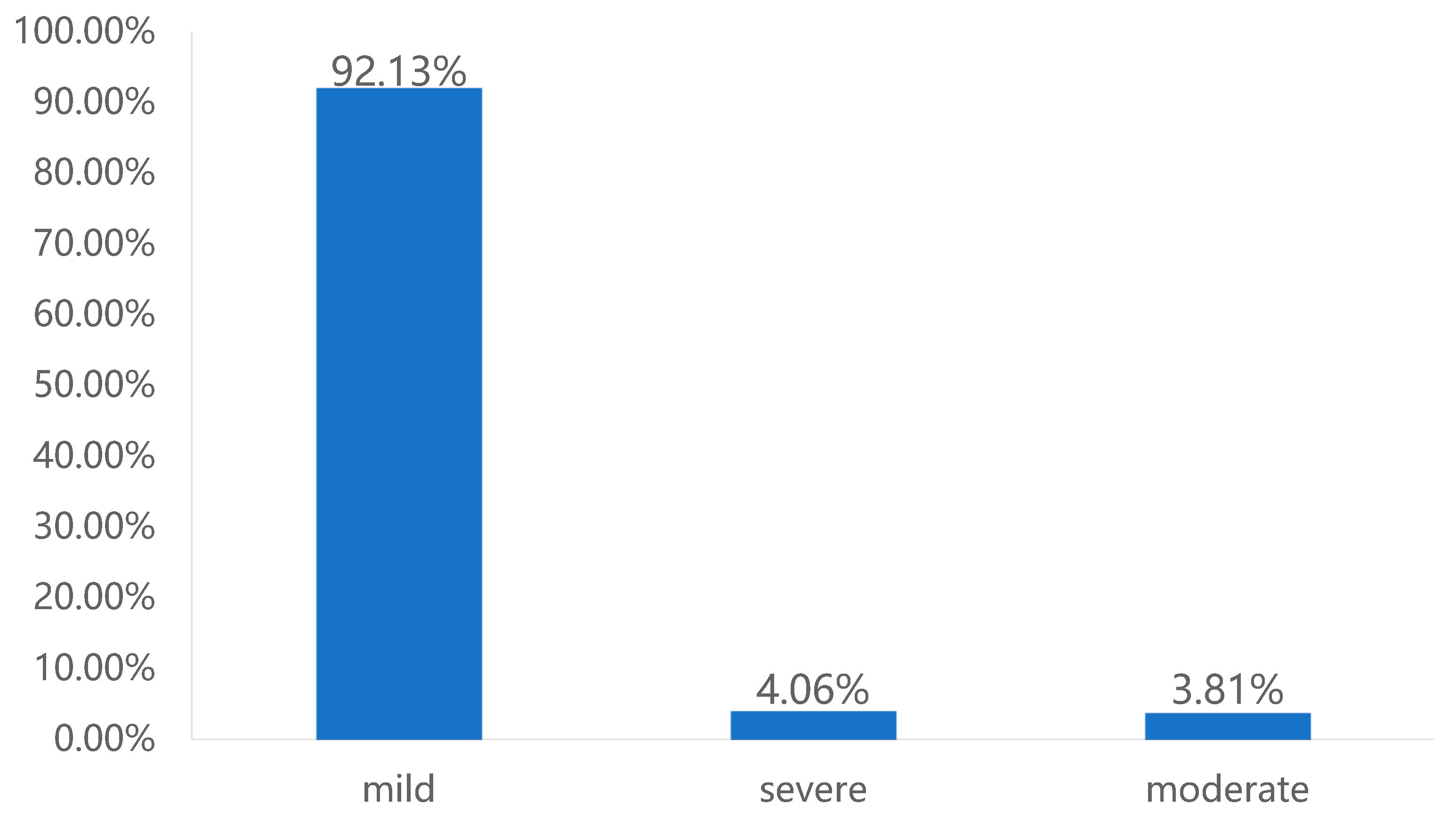
As shown in Figure 6, the vast majority of accidents are mild, with a proportion as high as 92.13%. The severity of most accidents is relatively low. Severe accidents account for only 4.06%, and moderate accidents account for 3.81%. Although these two types of accidents account for a relatively small proportion, they still cannot be ignored. In particular, severe accidents may cause significant losses to traffic, people, and property.

As shown in Figure 7, the proportion of “CA” (California) is the highest, reaching 25.33%, followed by 16.23% for “FL” (Florida) and 5.94% for “TX” (Texas). The proportion of “R” (right side) is 81.78%, which is significantly higher than that of “L” (left side), which is 18.22%. The proportion of “Eastern” (Eastern Timezone) is the highest, at 47.22%, followed by 29.54% for “Pacific” (Pacific Timezone) and 17.98% for “Central” (Central Timezone). This is because the distribution of accidents is affected by factors such as the population density, traffic flow, road conditions, and climate conditions.

As shown in Figure 8, in terms of the wind direction, the proportion of “CALM” (calm wind) is the highest, reaching 13.74%, followed by 6.09% for “S” (south wind) and 5.48% for “W” (west wind). The wind direction has a relatively minor impact on the occurrence of accidents, but strong winds may affect vehicle stability as well as drivers’ vision and judgment. Regarding the sunrise and sunset situations, the accident proportion during “Day” (daytime) is 69.85%, which is significantly higher than that during “Night” (night-time), which is 30.00%. The distribution of accidents during the day and at night is affected by factors such as the visibility, traffic flow, and driver behavior. During the day, although the visibility is good, drivers’ attention may be distracted. At night, the low visibility and drivers’ tendency to feel tired and sleepy increase the risk of accidents. Under civil twilight, the proportion of “Day” (daytime) is 74.19%, which is higher than that of “Night” (night-time), which is 25.65%. The change in lighting conditions during this period will affect drivers’ vision and judgment, and traffic flow and driver behavior are also different from those in other periods. Similarly, under nautical twilight, the proportion of “Day” (daytime) is also the highest, reaching 79.12%, which is higher than that of “Night” (night-time), which is 20.73%. Its special lighting conditions may also affect drivers’ vision and judgment on road traffic, and increase the risk of accidents.

As shown in Figure 9, in terms of the road roughness when the accidents occurred, the proportion of “FALSE” (no roughness) was as high as 99.96%, while that of “TRUE” (with roughness) was only 0.04%. The road roughness can affect the vehicle handling performance and driver comfort, increasing the risk of accidents. In the case of road intersections, the proportion of “FALSE” (non-intersection) was 93.13%, which was higher than that of “TRUE” (intersection), which was 6.87%. Most of the accidents happened on sections that were not at intersections, possibly due to high vehicle speeds or drivers’ lack of concentration. Regarding traffic calming measures, the proportion of “FALSE” (without traffic calming measures) was as high as 99.94%, and that of “TRUE” (with traffic calming measures) was only 0.06%. The implementation of such measures is affected by factors like the road types, surrounding environments, and traffic flows. In densely populated areas, they can reduce vehicle speeds to ensure the safety of pedestrians. On sections lacking these measures, vehicle speeds may be relatively high, increasing the risk of accidents. In the situation of traffic lights, the proportion of “FALSE” (without traffic lights) was 92.21%, which was higher than that of “TRUE” (with traffic lights), which was 7.79%. Most of the accidents occurred on sections without traffic lights. Traffic lights can regulate the traffic order and reduce accidents, and they play a particularly important role at intersections, where accidents are prone to happen.

3.2. Data Preprocessing

Due to the serious problem of data imbalance in the original data, this study performed under-sampling and over-sampling on “Severity”.

First, perform under-sampling on samples with “Severity” as mild. Use the sample function of the numpy library in Python3.11 to randomly select 80,000 pieces from many samples with the “Severity” as mild to reduce the number of such samples. In addition, perform over-sampling on those samples with the “Severity” as moderate and severe, respectively. For those samples with the “Severity” as moderate, use the resample function of sklearn in Python3.11 to increase the sample number to twice that of the original with the replacement. Perform the same over-sampling operation on those samples with the “Severity” as severe. Finally, combine the samples with the “Severity” as mild after the under-sampling and the samples with the “Severity” as moderate and severe after the over-sampling through the pd.concat function to create a more balanced data structure for the subsequent model training, with the hope to improve the key evaluation indicators, such as the accuracy and recall rate, of the classification prediction model.

To optimize the data quality to adapt to the subsequent model training, this study also performed missing value processing. Due to the large amount of data, this study deleted rows containing missing values so to ensure the integrity and accuracy of the data.

Encode categorical variables [41]. Determine the following features as categorical variables: [‘Side’, ‘State’, ‘Timezone’, ‘Weather_Condition’, ‘Wind_Direction’, ‘Sunrise_Sunset’, ‘Civil_Twilight’, ‘Nautical_Twilight’, ‘Astronomical_Twilight’]. Create and fit the LabelEncoder for each categorical column so to convert the categorical values into numerical codes.

Standardize the numerical features [42]. Determine the following numerical feature columns: [‘Distance(mi)’, ‘Temperature(F)’, ‘Wind_Chill(F)’, ‘Humidity(%)’, ‘Pressure(in)’, ‘Visibility(mi)’, ‘Wind_Speed(mph)’, ‘Precipitation(in)’]. Use StandardScaler for the standardization processing to make the different features have similar scales and distributions, which helps to improve the training efficiency and stability of the model.

4. Prediction Process

4.1. MLP Preliminary Prediction

This study took the lead in using the multi-layer perceptron (MLP) to conduct preliminary predictions and integrated the prediction results as new features into the source data. By incorporating the prediction results of the MLP to strengthen the depth of the feature expression, information was injected into the subsequent integrated prediction, thereby improving the upper limit of the model’s performance.

When constructing the MLP model architecture, a reasonable layout of the input layer, multiple hidden layers, and the output layer was set to complete the three-class classification task. The ReLU activation function was enabled in the hidden layer. Its advantages lie in effectively avoiding the problem of vanishing gradients, accelerating the convergence rate of the model, enhancing the nonlinear fitting efficiency, accurately capturing the complex feature interaction relationships, and deeply mining the potential patterns in the data, thus laying a solid foundation for accurate prediction. The softmax activation function was adapted in the output layer, which was in line with the characteristics of the multi-class classification tasks. It smoothly converted the model’s output into the probability distribution of each category, met the requirements of the multi-category judgment of the severity of traffic accidents, and ensured that the prediction results were accurate, reliable, and in line with the actual situation.

In the model initialization stage, the model structure was carefully determined according to the feature dimension of the input data to ensure that the architecture was delicately adapted to and synergized with the data features. The Adam optimizer was selected. Its excellent ability to adjust the adaptive learning rate could dynamically optimize the update step size according to the characteristics of the gradient, efficiently balance the convergence speed and stability throughout the training process, avoid falling into the trap of local optima, accurately locate the global optimal solution, and promote the model learning to reach an ideal state. Through experiments and fine-tuning, the learning rate was precisely set to 0.001. On the premise of ensuring convergence, it avoided the drawbacks of the parameters skipping the optimal region caused by too-large gradients or slow convergence caused by too-small gradients, ensuring a win–win situation for the training efficiency and effectiveness. The CrossEntropyLoss function was adopted as the loss function. This function could accurately measure the difference between the predicted probability distribution and the true label in multi-class classification scenarios, was in line with the essence of the classification task of the severity of traffic accidents, effectively guided the model to learn accurately and optimize the parameters, and improved the prediction accuracy and reliability. The evaluation indicator focused on the accuracy because it intuitively reflected the proportion of samples correctly predicted by the model and was the core benchmark for measuring the overall prediction quality of the model. It provided clear guidance for the model performance evaluation and optimization, ensuring that the model could stably output high-quality results in the task of predicting the severity of accidents, and laid a solid and accurate data foundation for traffic management decisions.

4.2. Secondary Prediction with Multiple Models

In this experiment, the results preliminarily predicted by the MLP were added as new features into the source data so to provide guidance and reference for the subsequent secondary prediction models and to improve the relevant indicators of the model by combining the advantages of multiple models.

4.2.1. Decision Tree Secondary Prediction

When constructing the decision tree model for the secondary prediction, its maximum depth was set to be unlimited, aiming to deeply explore the complex feature correlations in the traffic accident data. The severity of traffic accidents is affected by the interaction of multiple factors such as the geography, weather, roads, and vehicle driving status, with intertwined relationships. The unlimited depth enabled the decision tree to comprehensively explore the deep logic of features, accurately capture the subtle differences in the accident occurrence mechanism, avoid truncating critical information due to the limited depth, ensure a complete mapping and in-depth insight into the complex data features, and improve the accuracy of discriminating the severity of the accidents.

The minimum number of samples required for internal node splitting was set to two, and the minimum number of samples for leaf nodes was set to one, which was in line with the unbalanced characteristics of the traffic accident data. Although the minority class samples (severe accidents) accounted for a small proportion, their key features were prominent. This setting prevents ignoring important feature combinations of the minority class due to strict requirements on the number of samples. Based on sufficient sample statistical information, it steadily expands the growth path of the decision tree, enhances the model’s sensitivity to samples of various categories, accurately depicts the mapping relationship between the accident features and severity levels, and strengthens the stability and discriminative accuracy of the model.

4.2.2. XGBoost Secondary Prediction

When constructing the XGBoost classifier, in this study, if there were too many trees, the model would easily fit the noise and local fluctuations in the training data, while too few trees would make it difficult to capture the complex feature patterns. Therefore, the number of trees in the model was set to 100, and the contribution degree of each tree was set to 0.1. This enabled the model to effectively learn the features and collaboratively optimize the prediction, avoid the accumulation of biases of a single tree and the risk of overfitting, achieve a delicate balance between the accuracy and generalization, and accurately capture the change trend and feature associations of the accident severity.

The maximum depth of the trees was limited to six layers, which was highly consistent with the characteristics of traffic accident data and the requirements for generalization. Traffic data usually have a high dimension and complex feature relationships. If the tree depth was too large, the model would easily become trapped in the details of the training data and overfit the accidental features in specific scenarios, thus weakening the generalization ability for new samples. With a depth of six layers, the XGBoost model was guided to focus on the core feature levels and common patterns in the data, accurately extract the key information, maintain a good generalization vitality, ensure the stable and accurate prediction of the accident severity under different traffic conditions, and improve the reliability and practicability of the model.

4.2.3. Random Forest Secondary Prediction

When creating the random forest classifier, the number of decision trees affects the stability of the model. If the number is small, the model is easily affected by a single tree, resulting in insufficient learning and large fluctuations in the prediction results. Although a large number of decision trees can reduce the variance, it will increase the computational load and the risk of overfitting. Through experiments, the number of decision trees was set to 100, achieving the best performance balance under the data size and feature dimension of this study. It can fully integrate the advantages of multiple decision trees, stably capture the feature patterns in the accident data, and improve the consistency and accuracy of the prediction.

The “gini” criterion was adopted to measure the importance of features and the quality of splitting. Given that traffic accident data contain multiple variables, and some of them are correlated, the “gini” criterion focuses on the improvement degree of the sample class purity of the child nodes after feature splitting, accurately screens out the key features to construct decision tree branches, suppresses the interference of irrelevant features, optimizes the learning path and structure of the model, and enhances the interpretability and prediction performance of the model.

The maximum depth of the trees was limited to six layers, which was carefully determined based on the complex structure of traffic accident data and the requirements for the generalization. If the depth is too large, the model is prone to overfitting the local details and noise in the training data, thus impairing the generalization ability of the model for new samples. With a depth of six layers, overfitting can be effectively curbed, guiding the model to focus on the core feature levels and common patterns, ensuring the accurate and stable prediction of the severity of accidents under different traffic scenarios, and improving the practicality and reliability of the model.

5. Prediction Results and Analysis

5.1. Comparison of Overall Results

As shown in

Table 3. Comparison results of the overall results.

Model	Precision	Recall	F1
Individual MLP	0.86	0.84	0.85
Individual XGBoost	0.82	0.77	0.79
MLP + XGBoost	0.90	0.90	0.91
Individual random forest	0.92	0.90	0.90
MLP + random forest	0.94	0.94	0.94
Individual decision tree	0.87	0.88	0.85
MLP + decision tree	0.91	0.92	0.91

, in terms of the accuracy, among the individual models, the random forest model has the highest accuracy of 0.92, followed by the MLP with 0.86, while the XGBoost model is relatively low at 0.82. In the integrated model, the accuracy of the MLP + random forest model reaches 0.94, which is the most outstanding. In terms of the recall rate, among the individual models, the random forest model has the highest recall rate of 0.90, followed by the decision tree model with 0.88. In the integrated model, the recall rates of the MLP + random forest and MLP + decision tree models are both 0.94 and 0.92, showing good performance. In terms of the F1 value, among the individual models, the F1 value of random forest model is 0.90, which is relatively high. In the integrated model, the F1 value of the MLP + random forest model is 0.94, with obvious advantages. Generally speaking, the performance of the integrated and improved model is better than that of the individual model. Among them, the MLP + random forest model has achieved good results in the accuracy, recall rate, and F1 value, indicating that combining the MLP with random forest can effectively improve the comprehensive performance of the model. The individual random forest performs relatively well among the individual models, but there is still a certain gap compared with the integrated model.

In order to more intuitively distinguish the performance improvement of the improved model, the heat maps of the confusion matrix of the model before and after the improvement are shown in Figure 10.

5.2. Comparison of Results at Different Severity Levels

As shown in

Table 4. Mild level.

Model	Precision	Recall	F1
Individual MLP	0.86	0.95	0.90
Individual XGBoost	0.84	0.90	0.87
MLP + XGBoost	0.92	0.94	0.93
Individual random forest	0.94	0.95	0.94
MLP + random forest	0.96	0.95	0.96
Individual decision tree	0.94	0.86	0.90
MLP + decision tree	0.96	0.90	0.93

, at the mild level, among the individual models, the decision tree and random forest models perform well in the accuracy, with both reaching 0.94. In the integrated model, the MLP + random forest and MLP + decision tree models are even more outstanding, with an accuracy of up to 0.96. In terms of the recall rate, among the individual models, the random forest model has the highest recall rate of 0.95. In the integrated model, both the MLP + XGBoost and MLP + random forest models reach 0.95. In terms of the F1 value, among the individual models, the F1 value of the random forest model is 0.94. In the integrated model, the F1 value of the MLP + random forest model reaches 0.96.

As shown in

Table 5. Moderate level.

Model	Precision	Recall	F1
Individual MLP	0.85	0.91	0.88
Individual XGBoost	0.83	0.77	0.80
MLP + XGBoost	0.95	0.95	0.95
Individual random forest	0.89	0.86	0.88
MLP + random forest	0.93	0.94	0.94
Individual decision tree	0.78	0.88	0.83
MLP + decision tree	0.92	0.94	0.93
Logistic Regression	0.43	0.21	0.28

, for the moderate level, in terms of the accuracy, the integrated models, the MLP + XGBoost and MLP + random forest models, perform outstandingly, with both being 0.95. In the individual model, the accuracy of the decision tree model is 0.89. In terms of the recall rate, in the integrated model, the MLP + random forest model is the highest at 0.94. In the individual model, the decision tree model is 0.88. In terms of the F1 value, in the integrated models, the MLP + XGBoost and MLP + random forest models are both 0.95. In the individual model, the decision tree model is 0.83.

As shown in

Table 6. Severe level.

Model	Precision	Recall	F1
Individual MLP	0.87	0.68	0.76
Individual XGBoost	0.75	0.65	0.70
MLP + XGBoost	0.86	0.82	0.84
Individual random forest	0.89	0.88	0.89
MLP + random forest	0.91	0.92	0.91
Individual decision tree	0.76	0.90	0.82
MLP + decision tree	0.82	0.91	0.86
KNN	0.66	0.71	0.68

, at the severe level, among the individual models, the random forest model has the highest accuracy of 0.89. In the integrated model, the accuracy of the MLP + random forest model is 0.91. In terms of the recall rate, among the individual models, the decision tree model has the highest recall rate of 0.90. In the integrated model, the MLP + random forest model is 0.92. In terms of the F1 value, among the individual models, the random forest model is 0.89. In the integrated model, the MLP + random forest model is 0.91.

In actual traffic, the number of mild accidents is relatively large. The prediction accuracy rate of the improved model for mild accidents can reach above 0.94, which indicates that the model can well capture the common feature patterns of mild accidents. By learning these features, the model can accurately classify mild accidents.

As for moderate and severe accidents, although their numbers are relatively small, the improved model can also achieve a relatively high accuracy rate after data preprocessing and algorithm optimization. This shows that the improved model can identify the key features related to moderate and severe accidents from the complex traffic data, such as bad weather, poor road conditions, overly long driving distances, and other factors, so as to accurately predict the severity of accidents.

By adding the “Moderate level” and “Severe level” to the existing models commonly used for accident prediction for comparison, it is once again proved that the improved model has good adaptability in prediction scenarios dealing with complex features.

5.3. Model Evaluation

To better evaluate the improvement level of the performance of the integrated–improved model proposed in this study, this study uses the ROC curve and PR curve to evaluate the model performance before and after the improvement. Meanwhile, a sensitivity analysis is conducted on the selected improved model with the best performance to evaluate the generalization ability of the model.

The ROC curve (Receiver Operating Characteristic Curve) takes the false-positive rate (False-Positive Rate, FPR) as the abscissa and the true-positive rate (True-Positive Rate, TPR) as the ordinate.

The AUC (Area Under the Curve) value: The AUC is the area under the ROC curve, and the value range is between zero and one. The larger the AUC value, the better the performance of the model. Among them, AUC = 0.5 indicates that the prediction ability of the model is the same as random guessing. An AUC close to one indicates that the model has a good discrimination ability.

Compare the ROC curves of different models as follows: If the ROC curve of one model is completely above that of another model, the former has a better performance than the latter.

As shown in Figure 11, the prediction ability of each model after the improvement is improved at all levels.

In traffic accident prediction, a higher AUC (Area Under the Curve) value indicates that the model can effectively distinguish accidents with different severity levels. From the perspective of actual traffic scenarios, the improved model can accurately judge the possibility of accidents and their severity levels based on various input traffic features, such as the weather, road conditions, and vehicle driving status, providing timely and effective decision-making support for traffic management departments.

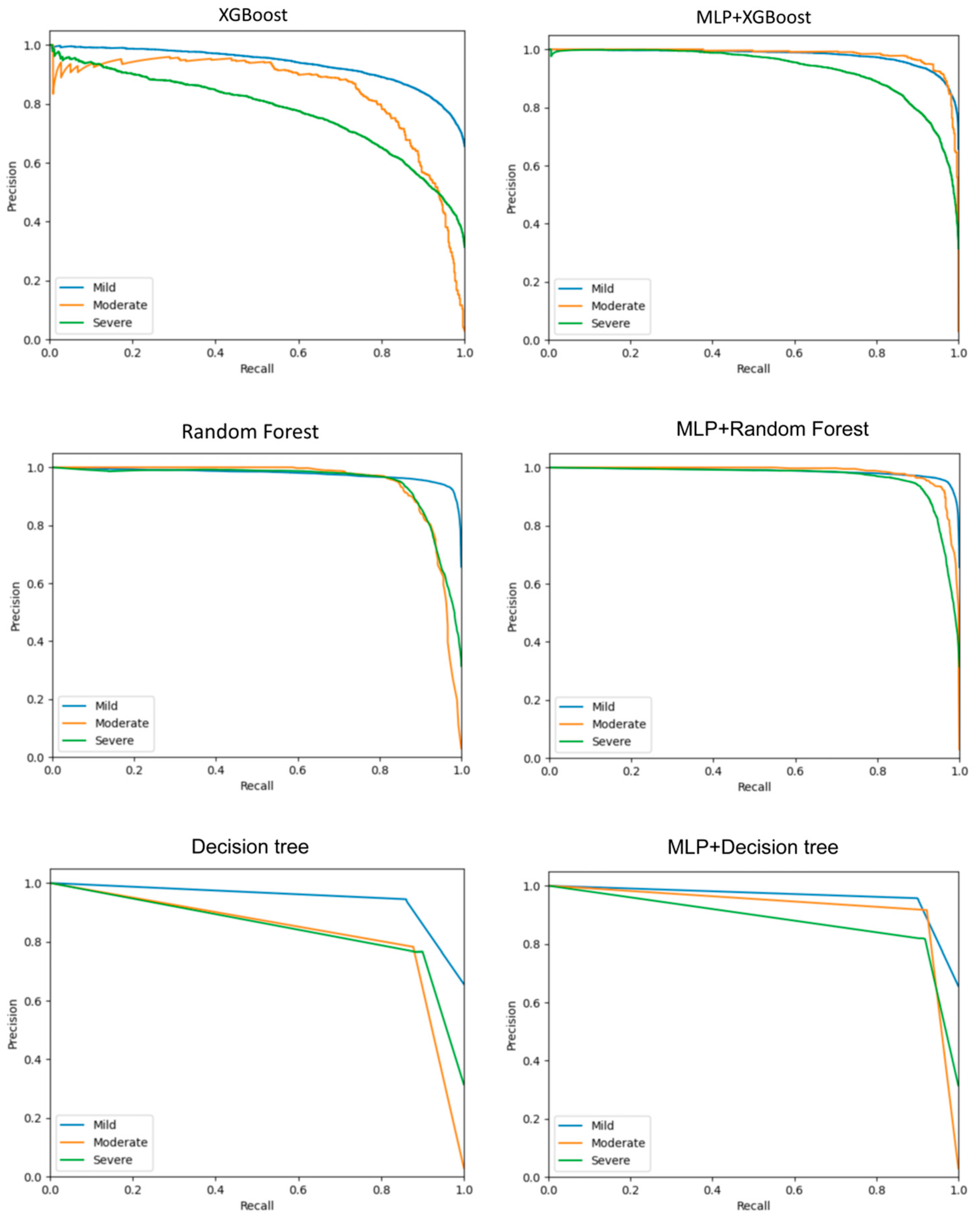
The PR curve (Precision–Recall Curve) takes the recall rate (Recall) as the abscissa and precision rate (Precision) as the ordinate.

The shape and position of the curve: The closer the curve is to the upper right corner, the better is the model performance. The average precision (Average Precision, AP): the AP is the area under the PR curve, which can comprehensively measure the precision performance of the model at different recall levels.

As shown in Figure 12, the comprehensive performance of the improved model is greatly improved compared with the original model.

At different severity levels, the integrated model generally shows better performance. In particular, the MLP + random forest model has excellent performance in the accuracy, recall rate, and F1 value at multiple levels. The individual random forest model also has good results at some levels, but, in general, the stability and comprehensive performance of the integrated model are more prominent.

The PR (Precision–Recall) curve evaluates the model performance from the perspectives of the precision and recall. In actual traffic scenarios, a high precision means that the probability is relatively high that an accident predicted by the model to be of a certain severity level actually occurs, while a high recall indicates that a relatively large proportion of accidents of that actual severity level are accurately predicted by the model. The improved model can not only accurately identify the real severe accidents but also reduce the misjudgment of accidents as severe ones, which can ensure that traffic rescue resources can be allocated to the places that truly need them in a timely and effective manner, and improve the efficiency of traffic emergency management.

Judging from the accuracy, recall, and other indicators of each model in predicting accidents of different severity levels, the combination of the MLP (multi-layer perceptron) and random forest is the most suitable for the severity prediction. Therefore, in this study, through the sensitivity analysis of the five features, namely, “Pressure (in)”, “Timezone”, “Humidity (%)”, “State”, and “Distance (mi)”, when the noise points are added to each feature with a multiple ranging from 0.8 to 1.2, the fluctuation range of the accuracy is less than 0.3%, as shown in Figure 13, which further confirms that this model has relatively strong stability.

6. Discussion and Conclusions

The results of this study offer valuable insights and prompt several important discussions. Firstly, the improved model, especially the MLP + random forest model, exhibited superior performance across various evaluation metrics compared to individual models. This demonstrates the effectiveness of combining different algorithms in capturing the complex relationships within the data. The synergy between the MLP’s ability to learn hierarchical representations and the random forest’s ensemble learning capability is evident. For instance, in terms of accuracy, the MLP + random forest model achieved an accuracy of 0.94, significantly outperforming most individual models. This indicates that the combination can better handle the diversity and complexity of the traffic accident data, reducing misclassifications and enhancing the overall prediction accuracy. However, it should be noted that individual models like the random forest also performed relatively well in some aspects. The random forest had an accuracy of 0.92 on its own, highlighting its own strengths in handling data, such as its ability to manage high-dimensional data and its robustness to noise. But when combined with the MLP, its performance was further improved, emphasizing the benefits of integration.

Meanwhile, the data imbalance in the original dataset, with the majority of accidents being of mild severity, was a significant challenge. By employing under-sampling and over-sampling techniques, a more balanced data structure was created. This had a positive impact on the model’s performance, particularly in terms of the recall rate and F1 value. For example, at the mild level, after the data preprocessing, the recall rates of the MLP + random forest and MLP + decision tree models reached 0.95 and 0.96, respectively, showing that the models can better identify the true-positive cases of mild accidents. This emphasizes the crucial role of appropriate data preprocessing in dealing with real-world datasets, where data imbalance is common. Without addressing this issue, the model might have been biased towards the majority class (mild accidents) and performed poorly in predicting the minority classes (moderate and severe accidents).

Finally, when looking at the performance at different severity levels, it is clear that the models’ performance varied. At the mild level, both individual models, like the decision tree and random forest, and the integrated models showed excellent accuracy, with values reaching 0.94 and above. This could be due to the relatively larger number of mild accident samples in the dataset, which allowed the models to learn the patterns more effectively. However, as the severity level increased to moderate and severe, the performance differences between the models became more pronounced. The integrated models, such as the MLP + XGBoost and MLP + random forest models, performed outstandingly in the accuracy and other metrics at the moderate and severe levels. This suggests that the integrated models are better able to capture the unique characteristics and patterns associated with different severity levels, perhaps due to the combined learning from multiple algorithms and the additional features provided by the MLP preliminary prediction. For example, at the severe level, the individual random forest model had an accuracy of 0.89, while the MLP + random forest integrated model achieved an accuracy of 0.91. The improvement in the accuracy shows that the integrated model can better handle the relatively rarer severe accident cases and make more accurate predictions. It also indicates that the combination of the MLP and random forest models can capture more subtle differences and relationships in the data related to severe accidents, which may not be fully captured by individual models.

In this study, we first employed under-sampling and over-sampling techniques to address the data imbalance issue in the traffic accident dataset. Then, we adopted a multi-stage integration strategy and integrated an improved machine-learning approach, which involved using the multi-layer perceptron (MLP) for the preliminary prediction and combining it with the decision tree, XGBoost, and random forest algorithms for the secondary prediction. The results showed that the improved model achieved remarkable performance. The “MLP + random forest” model, in particular, had an accuracy rate of 94%, outperforming the other models in terms of the accuracy, recall rate, and F1 value. Moreover, by adding certain fluctuations to part of the data and further conducting a sensitivity analysis on this model, it was once again confirmed that the model has good stability and adaptability.

This research has significant theoretical and practical implications. Theoretically, it enriches the methodologies of machine learning in data preprocessing, especially in handling data imbalance, missing values, categorical variable encoding, and numerical feature standardization. The application of these techniques provides valuable references for future studies. The constructed improved machine learning model, particularly the “MLP + random forest” integrated model, expands the application scope and theoretical boundaries of machine learning algorithms. In practical applications, the findings of this research carry extensive potential in the field of intelligent driving and provide a scientific foundation for traffic planning and management. In terms of intelligent driving integration and safety strategy optimization, it is crucial to strengthen the deep integration with vehicle networking technology. By obtaining information in real-time through the vehicle network and interacting with the prediction model, accurate risk assessments and early warnings can be achieved. For example, multi-level early-warning signals can be issued in advance, personalized driving suggestions can be provided, and avoidance route planning can be optimized. A dynamic safety strategy adjustment system should be developed based on the prediction model, which automatically adjusts vehicle safety configuration parameters according to the real-time risk level, thus providing comprehensive protection for intelligent driving. Furthermore, by analyzing the relationship between accidents and urban layout, land use, as well as transportation infrastructure construction, the functional zoning in urban planning can be reasonably adjusted, the road network layout can be optimized, traffic buffer areas can be increased, and reasonable signal lights can be set. These measures will optimize the transportation environment from a macro-level and reduce potential accident factors. Additionally, expanding the application of prediction models to the field of education and training, combining virtual reality and augmented reality technologies to develop simulation training systems, can provide drivers with immersive experiences to enhance safety awareness and skills, thereby reducing the incidence of accidents from the source.

In future research, we will further collaborate with sociologists to integrate human behavior and socio-cultural factors into the models. This will further improve the prediction accuracy and provide robust support for traffic safety management. Additionally, the relationship between traffic flow and accidents will be further explained. In the future, we will conduct a special study on traffic flow fluctuation scenarios, such as the transition period between morning and evening rush hours and off-peak hours in the city. It is hoped that the decision threshold can be adaptively adjusted according to the real-time traffic flow characteristics. By conducting the real-time learning of traffic flow-related features (such as the rate of change in vehicle speed and the congestion index of road sections), potential risk factors can be captured in a timely manner, and stable and reliable support can be provided for accident prediction in different traffic flow scenarios.