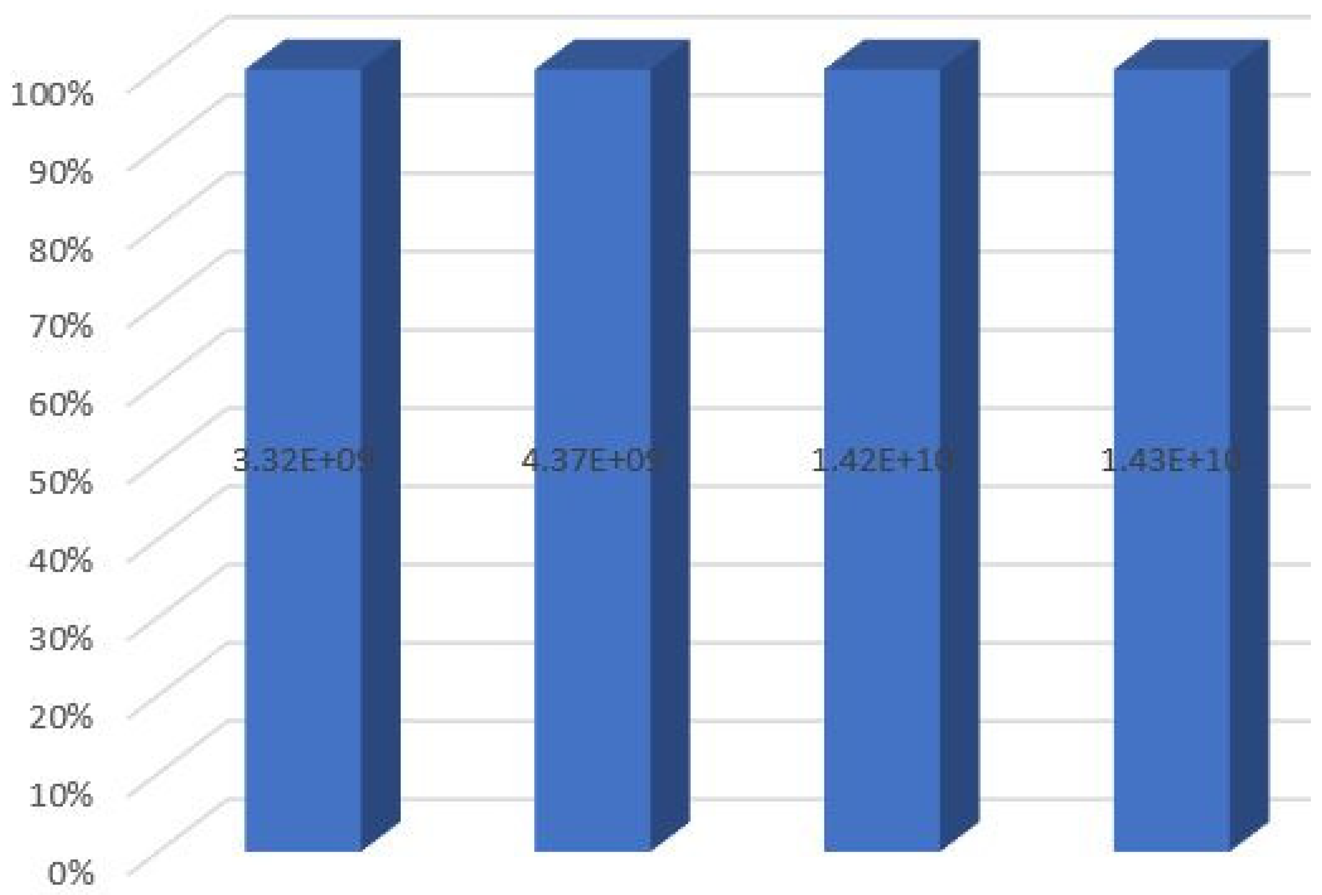
Abstract
Supply chain management and distribution network design has attracted the attention of many researchers in recent years. The timely satisfaction of customer demands leads to reducing costs, improving service levels, and increasing customer satisfaction. For this purpose, in this research, the mathematical programming models for a two-level distribution network including central warehouses, regional warehouses, and customers are designed so that several products with definite demands in multiple periods are distributed from central warehouses to customers. In this problem, two objective functions are considered. The first objective function seeks to minimize the costs of establishment, transportation, inventory, and shortage, and the second objective function attempts to maximize the satisfaction level corresponding with the supply rate of different goods for numerous customers. The presented models include the basic model, inventory-based model, multi-period inventory-based model, and multi-period inventory-based reverse logistics model. The validation and applicability of the proposed models were demonstrated by implementation in a real case study of the automobile industry. The LINGO software 20.0 was used to solve the models. The results show that incorporating the inventory management policies into the basic model and converting from a single-period to a multi-period reverse logistics model will significantly increase company profitability and customer satisfaction.
1. Introduction
In the present world, organizations are facing new opportunities and threats, which result from undergoing constant changes in the intra-organizational, inter-organizational, and international business environments [1]. The changing environmental conditions are so influential in the intra-organizational conditions that even small companies are affected by the fluctuations in the global economy [2]. On the one hand, organizations can create new opportunities and competitive advantages by properly utilizing various sciences and technologies that simultaneously progress consistent with the business environment [3]. Appropriately applying scientific theories to practical problems can lead to solving the new problems of organizations [4]. This is the point under consideration in the current study. The current research took ISACO company into account as a case study. ISACO, as the provider of after-sales service company of Iran Khodro Industrial Group, is the largest car manufacturer in the Middle East, which has an extensive commercial and service network to provide proper services to the customers and buyers of Iran Khodro products. Although this expansion has created a competitive advantage for this company compared with other domestic and foreign competitors, it has created some threats, too. The threats that have plagued most of the large companies cause the continuation of the previous strategies not being able to solve the problems. At the present time, ISACO has only one central warehouse in Tehran, which supplies the demands of the authorized company representatives, who are in charge of providing the services directly to the owners of Iran Khodro automobile products via this central warehouse. Investigating the company’s strategic index trend in the last few years indicates that some of the indices, including the market share of spare parts, have declined, and some indices such as the customer satisfaction level have not increased, and the existing satisfaction level does not guarantee the continuation of a successful presence in the market. Considering the separation of the supply and distribution system of parts and spare parts demanded by customers and the collection system of scrap parts and the existence of merely one central warehouse in Tehran (the central office of ISACO) to supply the increasing demands of customers of Iran Khodro products and subsequently; the demand increase in the authorized representatives scattered across the country; and considering the highly significant goals as to expanding the market share and increasing customer satisfaction, of the most important objectives in this company are to define a model to integrate the mentioned dual goals (increasing customer satisfaction and reducing costs) in such a way that it becomes possible to consider the two activities, i.e., parts distribution and scrap parts collection as a whole. Meanwhile, regarding the existence of a highly competitive environment in this industry in recent years and the foreign car manufacturers entering the scene, it is required to make some arrangements such as the possibility of returning unused parts to the authorized representatives and the possibility of exchanging unused parts with high-use and required parts. The significance of this matter made the category of green (reverse) logistics to be considered in this research so that objectives like increasing sale-accrued profit and recycling the scrap parts and helping to preserve the environment are considered.
Thus, based on the brief explanations provided, the research subject is designing a new system for spare parts distribution to authorized representatives across the country in a way that can simultaneously increase the profitability of the ISACO company and Iran Khodro Industrial Group as well as customer satisfaction level. In the present study, several scenarios and methods (assuming non-probabilistic, single- or multi-period data) have been presented, and the final model has undergone changes and modifications consistent with each scenario.
In the market share section as the company’s strategic index, despite the existence of a broad network of representatives, which has doubled since 2003—and currently their number is more than 750 representatives—the company’s market share has gradually declined. Despite exerting a direct effect on the company’s profitability, this index also has a meaningful impact on customer satisfaction levels. In the index of customer satisfaction out of the parts supply since 2008, the company’s measures could not lead to a proper increase in this index. Analyzing other indices, such as the percentage of unmet orders, transportation costs, storage costs, faulty parts rate, and operational parameters and the reports about parts shortage in the representatives, indicated the problems existing in the company’s distribution system. Under such conditions and considering the entry of new competitors, it is a must to revise the company’s macro-mission, i.e., the parts distribution system.
One of the main contributions of the present research is considering the two objectives of increasing customer satisfaction and reducing costs in the proposed mathematical model. In addition, the two activities of distributing parts and collecting used parts are taken into account. Moreover, the possibility of returning the unsold parts from the representatives and also the possibility of replacing the unsold parts with high-demand auto parts are considered in the model. In other words, regarding the reverse logistics concept, goals such as increasing profit from sales and recycling used parts to help preserve the environment are included in the presented model.
Therefore, the study aims to guarantee the survival and profitability of the company because failing to quickly and correctly make decisions will result in threats and irrecoverable losses. The present research pursues the goals to present a practical model to achieve the following:
- To optimize the transportation system in the ISACO company.
- To cut down transportation costs.
- To increase customer satisfaction by increasing the supply of customer demands.
- To allow the customers to return unused parts (which are not used by customers due to seasonal variations or environmental changes and market fluctuations.
- To collect and dispose or recycle the stock parts.
2. Literature Review
2.1. A Review of the Literature on Distribution Systems in Supply Chain Management
Liou et al. [5] presented a supply chain design model including factories and warehouses considering the deterministic demands of customers for different types of products. Their model seeks to make decisions on locating factories and warehouses and determining the amount of each product in each shipment with the aim of minimizing total costs. Two heuristic methods of Lagrangian relaxation and Simulated Annealing (SA) have been used to solve the model. The Lagrangian relaxation method is better than the other methods in terms of computational time and the quality of the solutions for medium- and large-size problems. On the other hand, the SA algorithm gained better solutions for small-size problems with higher computational time. Scott et al. [6] addressed the problem of locating several new factories with the aim of minimizing costs so that each factory serves several demand zones. The decision variables include the number of established factories and their locations and determining the demand zones so that the zones do not overlap with each other, and the demands are fully satisfied.
Dweiri et al. [7] first ranked warehouses based on the level of service required by customers using the AHP method. Then, they developed a mathematical model to maximize the customer satisfaction level considering the deterministic demand values and constraints such as the minimum allowed inventory amount for open warehouses and the number of warehouses. In addition, it was assumed that the demand of the customers must be fully met, and the amount of inventory must be fully distributed among the customers. In this way, a decision should be made regarding the opening of warehouses and the inventory level of each one. Mogeni et al. [8] designed a logistics system including several production centers, warehouses (distribution centers), and customers with uncertain demands with the aim of fulfilling total demands and minimizing logistics costs considering the required service levels. The model contains constraints related to travel time, capacity, speed, type, and the number of vehicles.
Muangpan et al. [9] declared that using information in a systematic way would help reverse logistics networks for recyclable materials. Brusset and Teller. [10] proposed a model for inventory control including determining the economic order amount, order point, and assurance inventory at the same time as locating facilities in the design of the distribution network with the aim of minimizing costs. The investigated supply chain included a production factory and a few warehouses with limited capacity, and each warehouse had a specific service level. The results showed that the presented model caused a significant reduction in costs compared to the traditional methods. Ribeiro et al. [11] examined supply chain management (SCM) from two different viewpoints including purchase and supply as well as transportation and logistics. From the viewpoint of purchase and supply, the evolution of SCM is defined by the efforts of manufacturers to integrate activities and partnerships with suppliers for more effective and efficient management of purchase and supply activities with the short-term goal of reducing production time and inventory level and increasing productivity together with the long-term goal of maximizing customer satisfaction level, market share, and the profit of stakeholders and improving performance. From the viewpoint of transportation and logistics, wholesalers/retailers attempt to integrate logistics activities and partner with logistics companies to manage transportation and distribution activities more effectively with online inventory management aiming to reduce transportation costs and demand uncertainty. Heidari et al. [12] investigated the supply chain network including suppliers, factories, and distribution centers to set up factories and distribution centers and determine the amount of the production and shipment of products with the goal of minimizing costs and environmental effects, and maximizing positive social impacts. The maximum number of factories and distribution centers that can be open and the capacity of factories, distribution centers, and suppliers are predetermined.
2.2. A Review of the Literature on Green Logistics in Supply Chain Management
Eydi et al. [13] investigated a multiple-period multi-echelon closed-loop supply chain network problem for product collection and shipment to determine an optimum number of facilities and their locations as well as the transportation modes. Antucheviciene et al. [14] proposed a model for a sustainable closed-loop supply chain problem aiming to identify the locations of facilities and optimize the materials’ flows under uncertain demands. Gholamian et al. [15] considered a sustainable multiple-period multi-echelon multi-product closed-loop supply chain problem aiming to minimize the total costs, the total waiting time, and the greenhouse gas emissions. Alinezhad et al. [16] addressed a sustainable multi-period closed-loop supply chain network problem with uncertain demand and return rates to maximize the total profits and customer satisfaction level. They solved the problem with the LP metric and Goal Attainment methods. Pazhani et al. [17] examined a multi-period closed-loop supply chain problem and exploited an integer relaxation method to obtain the optimal solutions. Nazari-Ghanbarloo and Ghodratnama [18] scrutinized the queuing system of the supply chain network with the aim of minimizing the total costs and time. Rabe et al. [19] studied a multiple-period capacitated facility location problem and utilized the Monte Carlo simulation approach for estimating the reliability levels and costs under random demands. Zarrat Dakhely Parast et al. [20] considered a sustainable closed-loop supply chain problem aiming to minimize the lost demands and total costs. Abdolazimi et al. [21] investigated a multi-period closed-loop supply chain network problem for minimizing the total costs and maximizing the number of on-time product deliveries together with the products’ quality, and solved the problem with the LP metric method.
Maliki et al. [22] investigated a multi-period facility location problem for a crisis situation considering uncertain demand to identify the locations of distribution centers with the aim of minimizing the costs and CO2 emissions. Gupta et al. [23] considered the logistics problem for determining the product order allocation to minimize the total costs. Bortolini et al. [24] investigated a sustainable supply chain network problem for minimizing the costs, stock levels, and greenhouse gas emissions. Mogale et al. [25] studied a multi-period sustainable closed-loop supply chain network problem considering various supply chain’s complexity. Al-Refaie and Kokash [26] addressed a sustainable reverse logistics problem under an uncertain environment with the goal of maximizing profit and positive social impact as well as minimizing CO2 emissions. Meidute-Kavaliauskiene et al. [27] modeled a multiple-period supply chain network under an uncertain environment for perishable products considering customer satisfaction, environmental impacts, costs, and procurement time. Allehashemi et al. [28] considered a closed-loop supply chain network with the goal of minimizing costs, maximizing quality, and minimizing CO2 emissions and solved it with the GAMS software 32.1.0. Abdi et al. [29] addressed a multi-period facility location-allocation problem considering uncertain demand with the goal of minimizing supply chain costs. Arab Momeni et al. [30] examined a sustainable closed-loop supply chain problem and solved the problem with the Epsilon Constraint (EC) method. Also, Varshney et al. [31] investigated a sustainable closed-loop supply chain network problem under uncertainty using the Pythagorean hesitant fuzzy programming. In addition, Xia et al. [32] modeled a reverse logistics network problem for end-of-life products under uncertainty and solved it with the NSGA-III algorithm.
3. Materials and Methods
Research scope
The scope of this research is the total requests for parts and spare parts from authorized representatives all over the country, which have been studied in different time periods. In terms of time, the design of the new distribution system is considered differently according to the type of products and the date of the start of product production in the Iranian market, and while examining the demand trends in different regions, more attention has been paid to the data of the recent years.
Data gathering tools
The required data were collected by using the information bank available in the ISACO company and holding specialized meetings with managers and experts in the development of the network of representatives and the field of commerce.
Analytical research model and data analysis method
Considering that the purpose of this research is to provide a practical innovative approach for the company, the operational research techniques were used to design a mixed integer linear programming model. Therefore, after designing an applicable model which is a linear, multi-objective, multi-product, multi-period, and integer model with binary variables, the model was implemented in the Lingo software 20.0 and then a decision was made according to the obtained results.
The steps of the research methodology
In this research, the features of the existing system were first identified. Then, by comparing with the other studied distribution systems, new scenarios were presented such as creating regional warehouses, increasing the number of central warehouses, and considering more parameters including inventory control issues in the decisions of regional warehouses.
According to the suggestions and scenarios presented, an appropriate model was proposed. Since each of the proposed scenarios needs to consider different assumptions and variables, a unique model was designed for each scenario. In addition, the Lingo software was used to obtain the optimal solution for each of the presented models, and finally, the appropriate suggestions were provided.
It should be noted that in designing a new model, various questions are usually asked, the purpose of which is to determine the data needed to form a suitable structure. Some of these questions are as follows:
1. What sites should use intermediate warehouses?
2. What should be the minimum amount of fulfilling the orders of representatives?
3. The selected intermediate warehouses should be fed from which central warehouses?
4. From which intermediate warehouses should the demanded goods of the customers be supplied?
5. What parameters should be considered in choosing the location of intermediate warehouses and central warehouses?
It is natural that the questions considered in the design of a new distribution system are more than the aforementioned questions, but these questions are the most basic questions that are raised as the initial basis of system design.
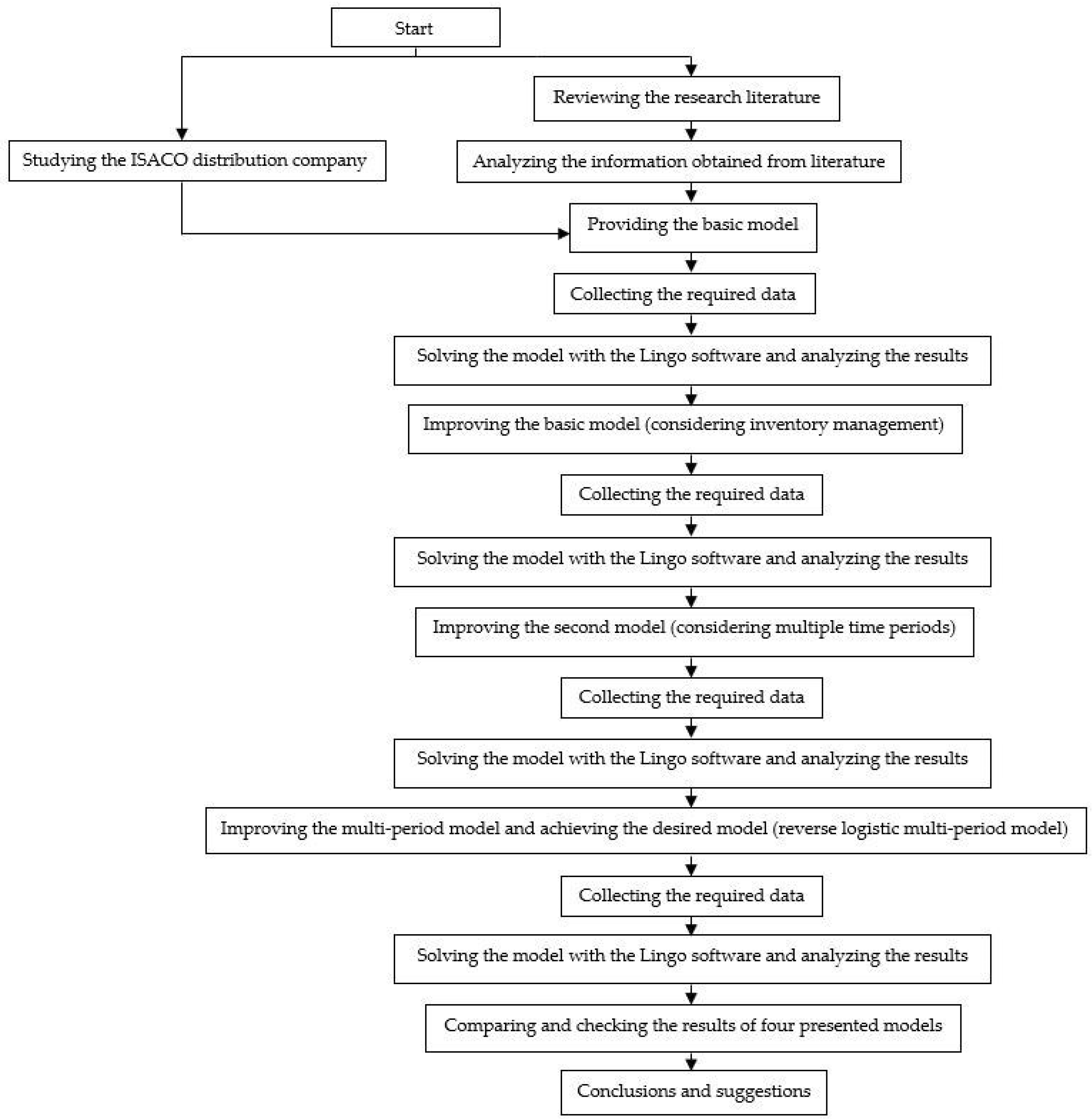
The steps of the research methodology are presented in Figure 1.
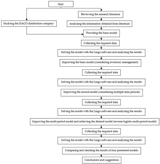
Figure 1.
The steps of the research methodology.
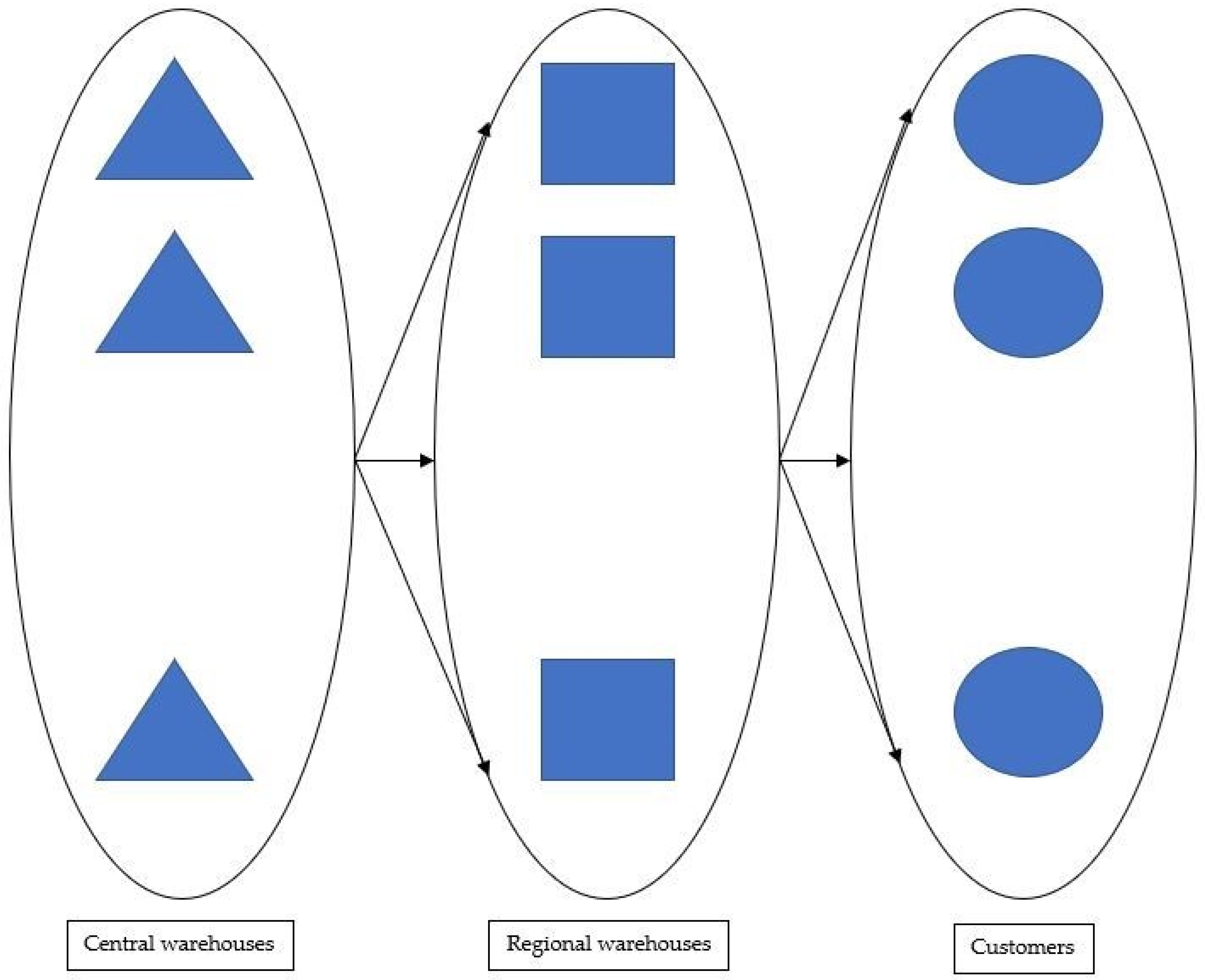
The structure of the new distribution system is depicted in Figure 2.
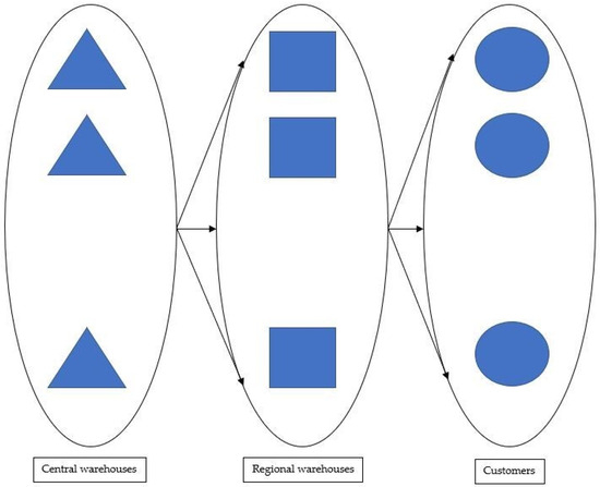
Figure 2.
The final structure of the studied distribution system.
Many real-world decision-making problems involve the simultaneous optimization of multiple objectives that are usually in conflict with each other. In single-objective optimization problems, we seek to find the “best” solution or decision, while in multi-objective optimization problems, there may be no solution that is optimal in terms of all the objectives. The proposed model is Mixed Integer Programming (MIP) with two objective functions. One of these objective functions is for minimizing the costs and the other is for maximizing the customer satisfaction, and these two objective functions contrast with each other so that increasing the value of one objective function results in decreasing the value of another. This problem has been solved through ideal programming and weighted methods.
Assumptions
A bi-level system has been considered for the study system, which includes central warehouses, regional warehouses, and representatives.
The goods transportation costs are obtained by the multiplication of the transportation cost per unit of goods by kilometer in the question distance, which is more accurate compared to fixed values.
The variable defined for the goods transfer from the central warehouse to the regional warehouse and also from the regional warehouse to the representatives is considered as a fraction. For example, half of the demand for the first type of goods may be delivered from the 3rd regional warehouse to the central warehouse, and the other half may be supplied from the 4th regional warehouse.
Notation
The sets, indexes, parameters, and decision variables are listed below.
Sets
L: The set of central warehouses, ;
M: The set of regional warehouses, ;
N: The set of representatives, ;
O: The set of goods, ;
F: The set of periods, .
Indexes
K: The central warehouse index;
j: The regional warehouse index;
i: The representative index;
t: The type of goods index;
p: The period index.
Parameters
: The demand of the ith representative for the tth goods during pth period;
: The capacity of the jth regional warehouse for the tth goods during the pth period;
: The capacity of the kth central warehouse for the tth goods during the pth period;
: The distance between the ith representative and the jth regional warehouse;
: The construction cost of the kth central warehouse;
: The construction cost of the jth regional warehouse;
: The construction and equipment cost of the recycling site for the jth regional warehouse;
: The inventory cost per unit of goods in the regional warehouse;
: The inventory cost per unit of goods in the central warehouse;
C: The shipping cost per unit of goods per kilometer;
g: The quantity (%) of return for returnable (unused) parts to the regional warehouse;
g′: The percentage of scrap parts that can be delivered to the recycling site;
s′: Higher purchase percentage after returning returnable (unused) parts;
: The shortage cost per unit of product shortage (back-order cost);
: The first objective function’s weight coefficient (costs minimization);
spit: The minimum supply quantity of tth goods type per ith representative during pth period with coefficient β.
Decision variables
: Variable 0 or 1, which is equal to 1 if the Kth central warehouse is constructed, and otherwise 0;
: Variable 0 or 1, which is equal to 1 if the jth regional warehouse is constructed, and otherwise 0;
: Demand percentage by the ith representative of the tth goods type delivered from the jth regional warehouse during pth period;
: Demand percentage by the jth regional warehouse of tth product type delivered from the kth central warehouse during the pth period.
Basic mathematical model
Subject to
The first objective function is for minimizing the costs of goods transportation, which includes the transportation of various types of goods between the regional warehouses and central warehouses ( and also between the regional warehouses and representatives . Besides, the construction costs of the regional warehouses and the construction costs of the central warehouses have been included in it.
The second objective function of the model is based on the representatives’ satisfaction according to meeting their needs ( and its goal is to maximize the representatives’ satisfaction whose optimal point is the one where the customers’ satisfaction per each item of goods reaches 1.
Based on Constraint 1 of the model, delivering any type of goods from the jth regional warehouse is allowed if this warehouse has already been constructed.
Based on Constraint 2, delivering goods from the kth central warehouse is allowed if this warehouse has already been constructed.
Based on Constraint 3, per each jth regional warehouse, the total amount of output goods per each type of goods t should be less than the capacity of the warehouse for the question goods.
Based on Constraint 4, per each kth central warehouse, the total amount of output goods per each type of goods t should be less than the capacity of the question warehouse.
Based on Constraint 5, per each type of goods t, a minimum level has been defined for satisfaction level with supply, the condition which should be met in all the equations.
Based on Constraint 6, the sum of the supply has to be higher than the demand quantity.
Based on Constraint 7, the satisfaction of the ith representative per tth type of goods has to be less than or equal to 1.
Based on Constraint 8, the sum of demands of the jth regional warehouse per tth type of goods has to be less than or equal to 1.
Finally, the type of decision variables is determined so that the variables are between 0 and 1 and the variables are 0 or 1.
Basic model development according to the real-world situation
The presented basic model paves the ground for implementing the proposed model and evaluating the intended solutions. As pointed out in the previous sections, building regional warehouses, increasing the number of central warehouses, and considering the costs of goods delivery and transportation besides considering customer satisfaction in the decision makings about transporting goods and locating the regional and central warehouses can be part of the policies and solutions that the basic model guarantees to supply. However, in order to make it more realistic and make the conditions closer to the real model, some new components were added to the model, which are presented in order.
Basic model development considering the inventory policies
Investigating several existing papers and studies, part of which are included in the literature review section, it has been found that one of the methods to ensure the modeling accuracy and compatibility with real-world problems is to add different components to the basic model. One of the significant issues in this discussion is inventory problems which we have decided to add to the basic model according to the knowledge we have about the real problem. In the following, the detailed illustration of inventory problems and the way to apply them in the basic model will be addressed. For this purpose, it is possible to consider inventory costs, including ordering costs, maintenance costs, and goods shortages in the basic model. Another matter which requires attention when designing the model is the policies and inventory control systems. In this matter, the ordering costs are almost negligible, and the transportation costs have been substantially taken into account; therefore, the costs considered in the inventory control system include maintenance costs, shortage costs, transportation costs, and order delivery (which were already included in the basic model). The ordering system is also a fixed period considered as proportional to the company’s quarterly (seasonal) ordering period.
Parameters and decision variables
Besides the parameters and variables employed in the basic model, the following parameters are added to the model regarding the addition of inventory management components.
: The inventory cost per unit of goods in regional warehouses;
: The inventory cost per unit of goods in central warehouses;
: The shortage cost per unit of goods shortage.
Mathematical model
Subject to the same constraints as the basic model: Constraints (1–12)
The first objective function is for minimizing the costs incurred by goods transportation, which includes the transportation of various types of goods between the regional warehouses and central warehouses plus the ones between the regional warehouses and representatives. The construction costs of the regional warehouses and central warehouses have also been included in it. Having completed the model at this stage, the goods storage costs in the central warehouse and regional warehouse and also the cost of inventory shortage have been indicated as the costs in the first objective function. The second objective function of this model is like that of the basic model.
Basic model development and conversion from a single-period to a multi-period reverse logistics model
With respect to the fact that most of the real-world problems are implemented during several time periods and some of the demand or supply may be transferred from one period to the next period, it is essential to consider this through designing the dynamic model. Thus, by applying some changes to the basic model and its variables, it becomes possible to implement the model for multi-period modes.
Sets
P: The set of periods .
The other sets are held similar to those of the basic mode.
Parameters and variables
The other parameters and variables are the same as the basic model and only the P index has been added to them as a sign of considering the period.
Here, the first objective function is for minimizing the costs incurred by goods transportation per period, which includes the transportation of all kinds of goods between the regional warehouses and central warehouses and between the regional warehouses and representatives. Moreover, the construction costs of regional warehouses and the construction costs of central warehouses have been included in it. The costs of goods storage in the central warehouse and regional warehouse per period, as well as the cost of inventory shortage per period, have been indicated as the costs in the objective function.
The second defined objective function is the same as the objective function of the previous mode, with the difference that it is considered for all the periods.
Subject to
Constraint (11)
Constraint (12)
Basic model development considering green logistics policy
The final model is presented as the following by considering the possibility of returning the goods which are returnable (unused) by the representatives and also centralizing the scrap parts recycling site in the regional warehouses and adding the cost of returning the scrap parts to the recycling site and the construction costs of this site to the first objective function.
Parameters and variables
: The cost of the construction and equipment of the recycling site for the jth regional warehouse;
g′: The percentage of scrap parts that can be returned back to the recycling site;
g: The quantity (percentage) of returnable (unused) parts to the regional warehouse;
S′: The percentage of higher purchases after turning back the unused parts.
The first objective function is for minimizing the transportation costs of all kinds of goods between the regional warehouses and central warehouses, the transportation costs of all kinds of goods between the regional warehouses and representatives, the transportation costs of all kinds of scrap parts to the recycling site, the construction costs of the regional warehouses, the construction costs of the central warehouses, the building cost of a recycling site, the inventory costs in the central warehouse and regional warehouse, and the cost of inventory shortage in each period which have been indicated as the costs in the first objective function.
The second objective function of the model is based on the representatives’ satisfaction with meeting their needs, and its goal is to maximize the representatives’ satisfaction, and its optimal point is the point where customer satisfaction reaches 1 per item of goods. This matter has been considered for all the periods and for returnable parts as well.
Subject to
Constraint (13)
Constraint (18)
Constraint (19)
Constraint (20)
Constraint (21)
Constraint (22)
Constraint (23)
Constraint (25)
Constraint (26)
Constraint (11)
Constraint (12)
4. Results
In addition to the basic model, three other models have also been introduced in this study. Hence, the outputs of the LINGO software are provided separately for each model.
Case Study
Iran Khodro Industrial Group was founded in 1977 as a manufacturing and distributing company of automobile parts and spare parts. Since its inauguration, the major activity of this company for twenty years has been focused on the supply and distribution of car parts manufactured by Iran Khodro Industrial Group. Like many large companies, ISACO is a loop of a specific supply chain with given duties. This supply chain is designed to pursue the goal of manufacturing and supplying cars to the end customers and has other duties as well. This supply chain network is made up of several interconnected loops so that automobile parts are primarily supplied by the parts manufacturers and are handed over to the SAPCO Company. Such parts are assigned to Iran Khodro Industrial Group by SAPCO, and Iran Khodro Industrial Group assembles the parts and manufactures the intended cars. Following that, ISACO provides after-sales services to customers through authorized representatives. The significant point in this chain is that Iran Khodro Industrial Group is the key connecting loop of the chain and other loops obey the policies of this key loop.
The existing distribution system in ISACO: Currently, this group has only one central warehouse in Tehran and possesses no other warehouses. This chain operates in a manner that the required goods are first supplied through domestic and foreign suppliers and stored in this warehouse and then according to the orders of the authorized representatives across the country, the goods are delivered. In the current system, there is no regional representative, and the cars are delivered to the representatives after being loaded from the central warehouse, and the parts required by the representatives are directly delivered to them.
The reasons behind applying the new system: The issue deserving attention is that the existing system is outdated and traditional, and at the present time, when the speed of modern technology service delivery is the distinguishing factor in global competition, it does not satisfy the current and future demands of the company; thus, it is a must to develop a befitting solution to get rid of this system’s drawbacks, some of which can be mentioned as the following:
- Very high transportation costs induced by long round-trip distances.
- High costs imposed on the company as a result of vehicle breakdown.
- Frequent troubles related to timely goods delivery (e.g., the cities located far from Tehran, the chances are high that the goods do not reach on time).
- To benefit from the full capacity of cars, it is required that the amount of the ordered goods reach a certain quantity and then the goods be delivered to the representatives, which leads to dissatisfaction among the representatives and losing the competitive market.
- The lack of order and prioritization in the current system.
- Not considering different scenarios in decision making.
- Not being able to return unused or low-use parts by the representatives.
- The lack of an integrated system for receiving scrap parts.
- Not able to implement strategic planning.
- Some of the expected merits of the new system are the following:
- Reducing the costs resulting from redundant transportation.
- Increasing the representatives’ satisfaction level due to goods’ timely delivery and increasing the power to supply the demanded goods and the possibility of returning low-use parts to the representative.
- Systematizing transportation system which curbs other nuisances.
- Increasing the flexibility of the system.
- Decreasing the risks such as the sensitive parts becoming faulty during long transportation or the possibility of vehicle breakdowns that impose losses on the company.
- Building regional warehouses and reducing the heavy costs of the central warehouse.
- Controlling the system better and the potential to constantly improve.
The expected distribution system: Considering several problems due to this old distribution system, some models have been presented to mitigate costs and build up the customer satisfaction level. As the first step, it is essential to determine the number of central warehouses. Accordingly, the first two locations have been considered as the central warehouses, which are Tehran and Bandar Abbas. The reason for selecting these two is that part of the goods used by the representatives are supplied from the Persian Gulf-based countries, which in the current system are first transported to Bandar Abbas and then to Tehran and following that, they are distributed from Tehran to other cities according to the demands of various cities; while some of the ISACO representatives are neighboring Bandar Abbas, it is consequently logical to eliminate redundant transportation by constructing a central warehouse in Bandar Abbas. Moreover, since there are numerous representatives and suppliers in Tehran and also due to the advantages of Tehran, such as being the capital and a densely populated city, it seems reasonable to build another central warehouse in this city. On the other hand, the proposed model aims to construct regional warehouses. Thus, several cities are considered as candidates for constructing regional warehouses, and the best locations are selected according to the objective functions.
It should be noted that the selection of candidate cities for intermediate warehouses is based on certain rules. For this purpose, the number of representatives and the populations of the desired cities throughout the country are considered. In addition, the representatives of each city are accumulated in the center of the province related to that city as it is unnecessary to pay too much attention to detail because this matter will increase the dimensions of the problem at hand and make it unsolvable by the Lingo software. Also, the locations of the intermediate warehouses are selected based on their population and closeness to the cities with the largest number of representatives; these cities are Isfahan, Tabriz, Khorram-Abad, Rasht, Shiraz, Kerman, Mashhad, and Sari. Subsequently, concerning the different types of cars manufactured by Iran Khodro Industrial Group, the products are divided into five groups. Then, all the representatives’ demand for each type of product is calculated so that we can calculate the total annual demand of all the cities in each province for each type of goods and consider the result as the total demand of each province.
With respect to the candidate cities for such warehouses, the capacity of the regional warehouses is calculated according to the proximity of the neighboring cities. For example, to calculate the capacity of a regional warehouse in Mashhad, first, the total demand for different items is calculated for the cities of Bojnoord (the center of North Khorasan province), Mashhad (the center of Khorasan Razavi province), and Birjand (the center of South Khorasan province) and then a quarter of this quantity is added to it as a three-month safety stock (SS) to reach the desired capacity. This operation is also performed to calculate the capacity of the central warehouses.
The results of solving the basic model
The basic model is able to evaluate and select suitable places for intermediate and regional warehouses as well as central warehouses from an expert point of view. This model, like a framework, is capable of adding different components to increase the accuracy of decisions.
It is necessary to simultaneously survey two parameters in order to estimate the model solution value and provide the final solution based on the values of these two parameters. These two parameters are the minimum level of supplying the customers’ demand (β) and the weight of the first objective function (α). The following Table 1 displays the computational results for the different values of these two parameters.

Table 1.
Computational results for different values of α and β.
Regarding the two objective functions conflicting with each other, the first objective function increase will result in the second objective function decrease. Figure 3 indicates the conflict of these two objective functions at β = 0.1
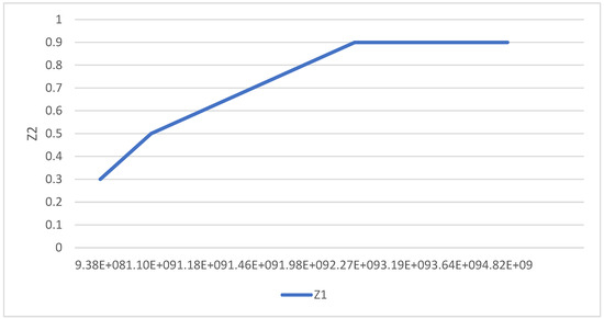
Figure 3.
Representation of two objective functions at minimum satisfaction level of 0.1.
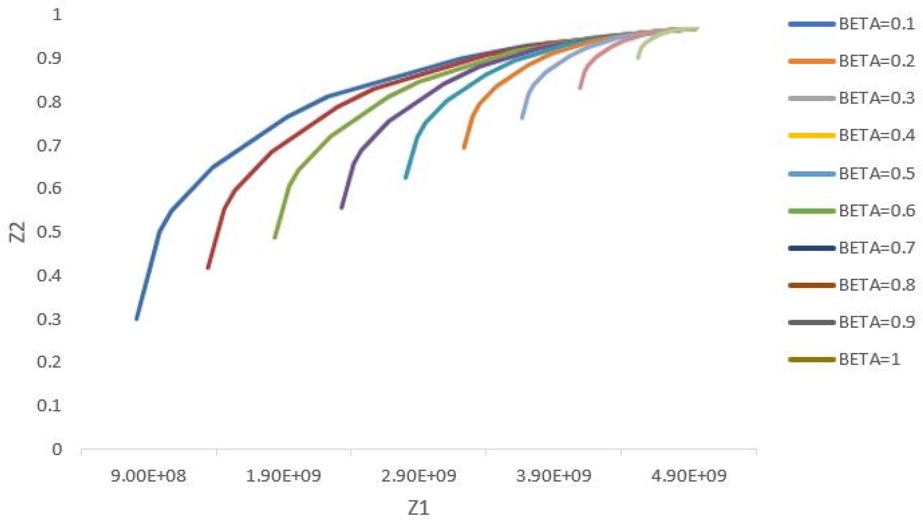
Considering that at different levels of minimum customer satisfaction, the above graph is different, the result will be different. The results of these computations are seen in Figure 4.
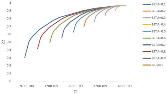
Figure 4.
Total costs versus customer satisfaction for different values of β.
With respect to the presented explanations, determining the appropriate and optimal value of the two parameters, i.e., α and β will be a problem. Therefore, it is required to provide a mechanism to optimally select these two parameters using heuristic methods.
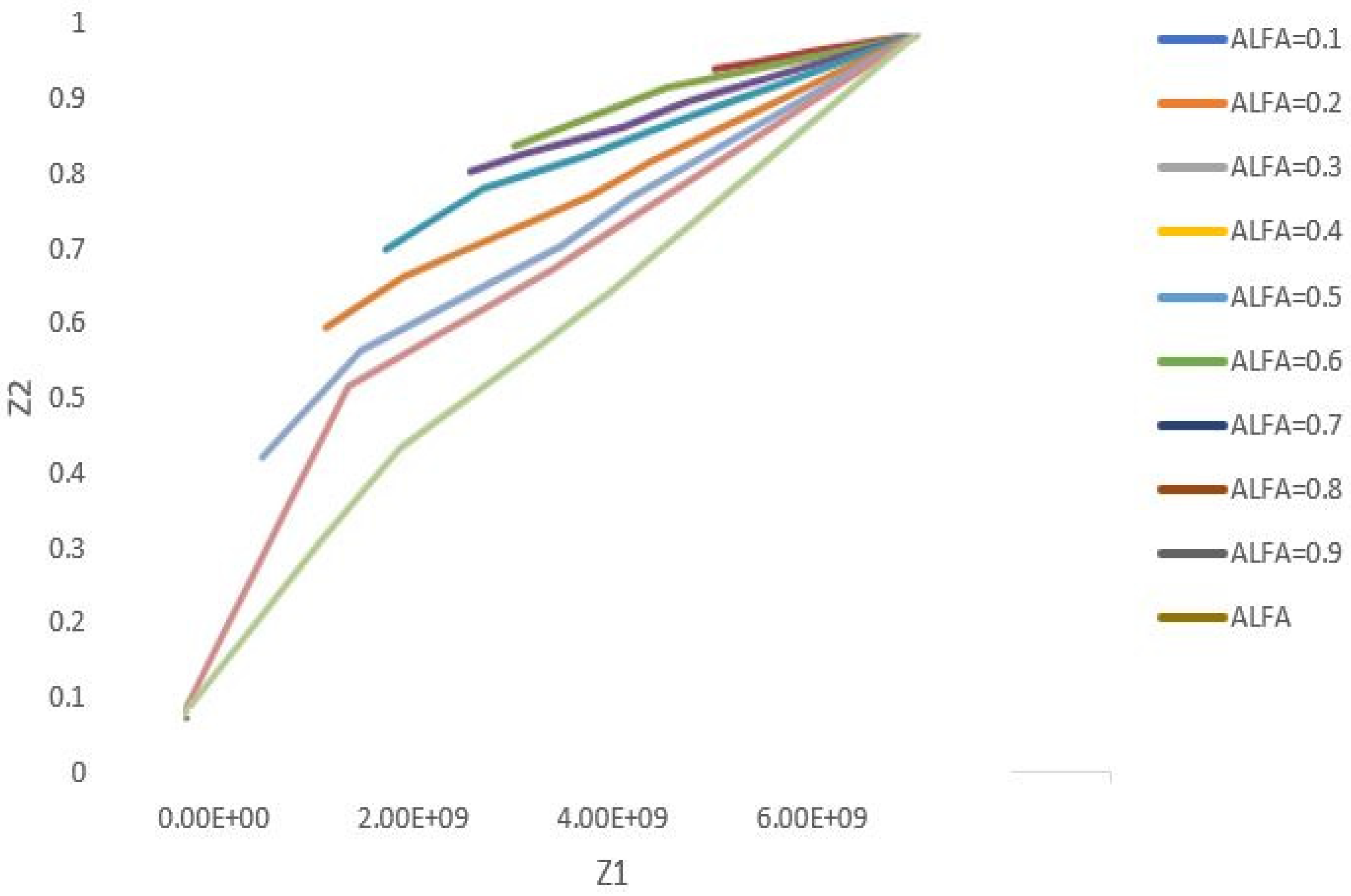
Figure 5 depicts the values of the two objective functions for different coefficients of the objective function and verifies that it is necessary to determine the optimal value by a certain method.
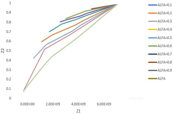
Figure 5.
Total costs versus customer satisfaction for different values of α.
A proposed method is to design a new function for determining the values of customer dissatisfaction as a percentage, and also the total cost divided by the maximum cost for the different values of α. Undoubtedly, when this new function has the minimum value, it gets close to the optimal mode.
Regarding the above cases, it is perceived that the senior management can measure the weighted coefficient of the first objective function by deciding at what minimum percentage they intend to meet the customers’ satisfaction, and based on this, the variables and parameters will also be determined. For instance, as a result of selecting β = 0.6, the coefficient of the first objective function (α) is determined as 0.7. Table 2 shows the results of the calculations and the outputs for the above parameters.

Table 2.
Model-extracted results based on α = 0.7 and β = 0.6.
The above table indicates that in the basic model, as a result of selecting β = 0.6 and the coefficient of the first objective function (α) equal to 0.7, the minimum cost is equal to 3.32 × 10⁹ Iranian Tomans, and the maximum customer satisfaction will be equal to 80% while both central warehouses have been selected for construction, and out of the eight proposed regional warehouses, only regional warehouses 6 and 8, that is, the cities of Kerman and Sari have been chosen for construction.
Basic Model Solution Results along with Inventory Management Policies
Considering the inventory management policies being added to the objective function, the model solution results are as follows: Given this matter that similar to the basic model, the two parameters of the minimum satisfaction level and the coefficient of the first objective function can have different values, it is required to do the computations for different values of these two parameters. The following Table 3 includes the computational results of the two objective functions.

Table 3.
Basic model computational results along with inventory management policies for different values of α and β.
Regarding the two objective functions that are opposite to each other, the first objective function increase will be accompanied by the second objective function decrease.
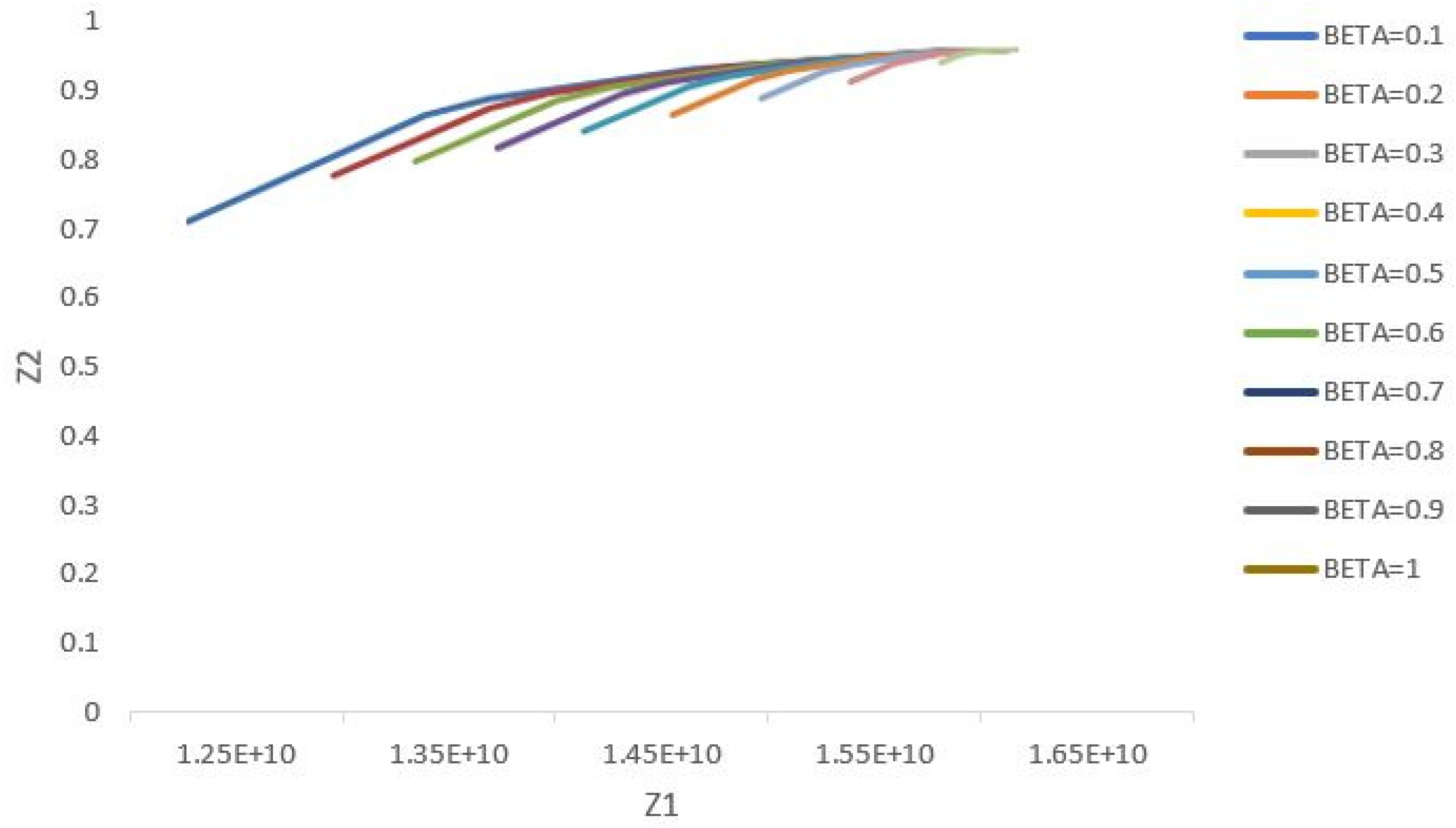
Given that at different levels of minimum customer satisfaction, Figure 6 has a different shape, and the results also differ, the computational results are given in Figure 7.
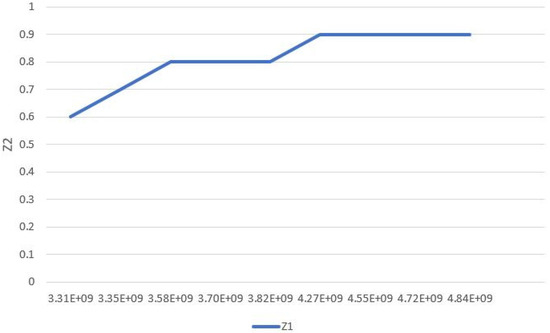
Figure 6.
Representation of two objective functions at minimum satisfaction level.
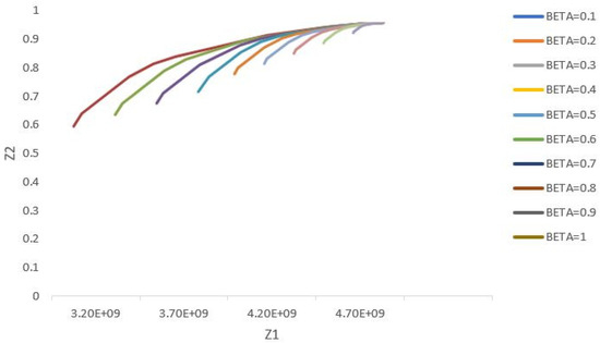
Figure 7.
Total costs versus customer satisfaction in basic model along with inventory management policies for different values of β.
Pursuant to the explanations provided so far, determining the suitable and optimal value of the two parameters β and α will be a problem. Therefore, it is required to develop a mechanism for optimally selecting these two parameters via heuristic methods.
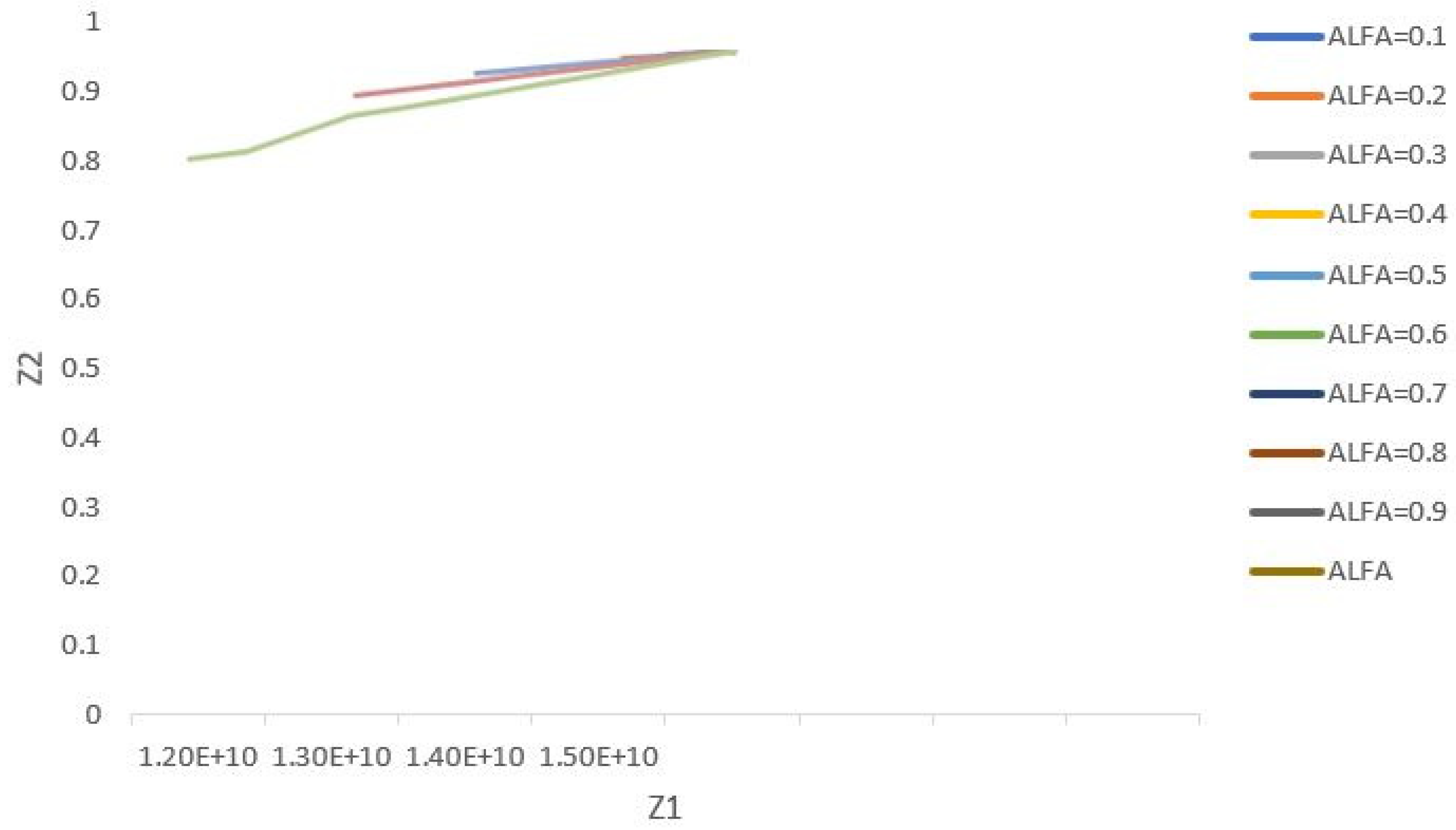
Figure 8 depicts the values of the two objective functions for different coefficients of the objective functions.
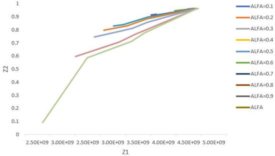
Figure 8.
Total costs versus customer satisfaction in basic model along with inventory management policies for different values of α.
Using the proposed method in the previous section, we set up a new function to measure the percentage of customer dissatisfaction and also the total costs divided by the maximum cost for the different values of α. It is clear that when this new function has the minimum value, it gets close to the optimal mode. Considering the above graph, it is discovered that the senior management can measure the weighted coefficient of the first objective function by deciding at what minimum percentage they intend to meet the customers’ satisfaction, and accordingly, the variables and parameters will also be determined. For example, as a result of the selection β = 0.6, the coefficient of the first objective function (α) is determined as 0.7. Table 4 shows the computational results and the outputs for the above parameters.

Table 4.
Model results based on α = 0.7 and β = 0.6.
The above table displays that by adding the inventory management policy to the basic model, as a result of selecting β = 0.6 and the coefficient of the first objective function (α) as 0.7, the minimum cost is equal to 4.37 × 10⁹ Iranian Tomans, and the maximum customer satisfaction will be equal to 92% while both central warehouses have been picked for construction, and out of the eight proposed regional warehouses, only regional warehouses 6 and 8, i.e., the cities of Kerman and Sari have been chosen to be built.
Basic Model Solution Results along with Multi-Period Policies
To estimate the model’s solution value, it is required to concurrently analyze the two parameters and present the final solution based on the values of these two. These two parameters are the minimum level of meeting the customers’ demands (β) and the first objective function’s weight (α). Table 5 displays the computational results for the different values of these two parameters.

Table 5.
Computational results of multi-period model for different values of α and β.
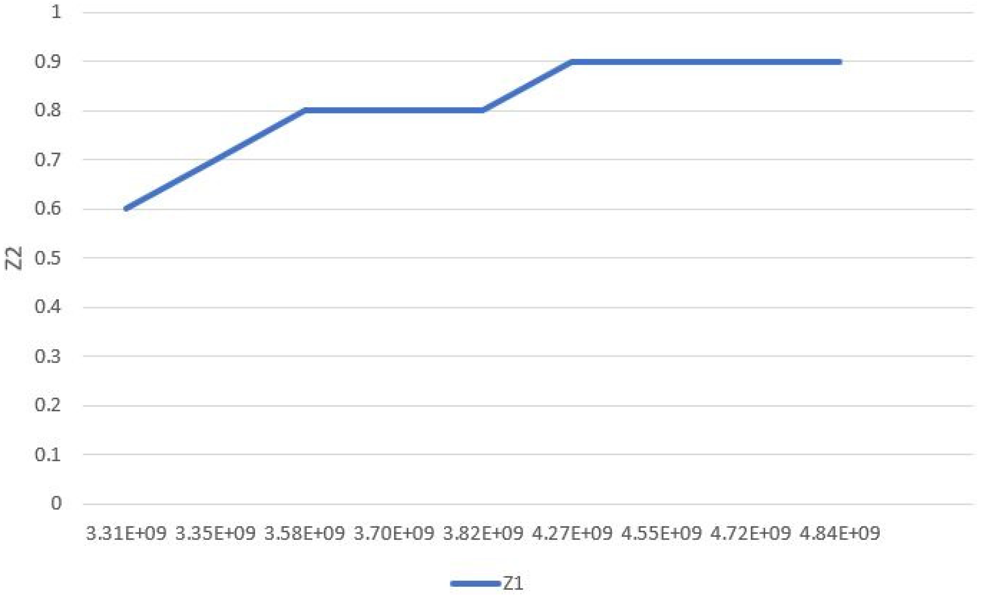
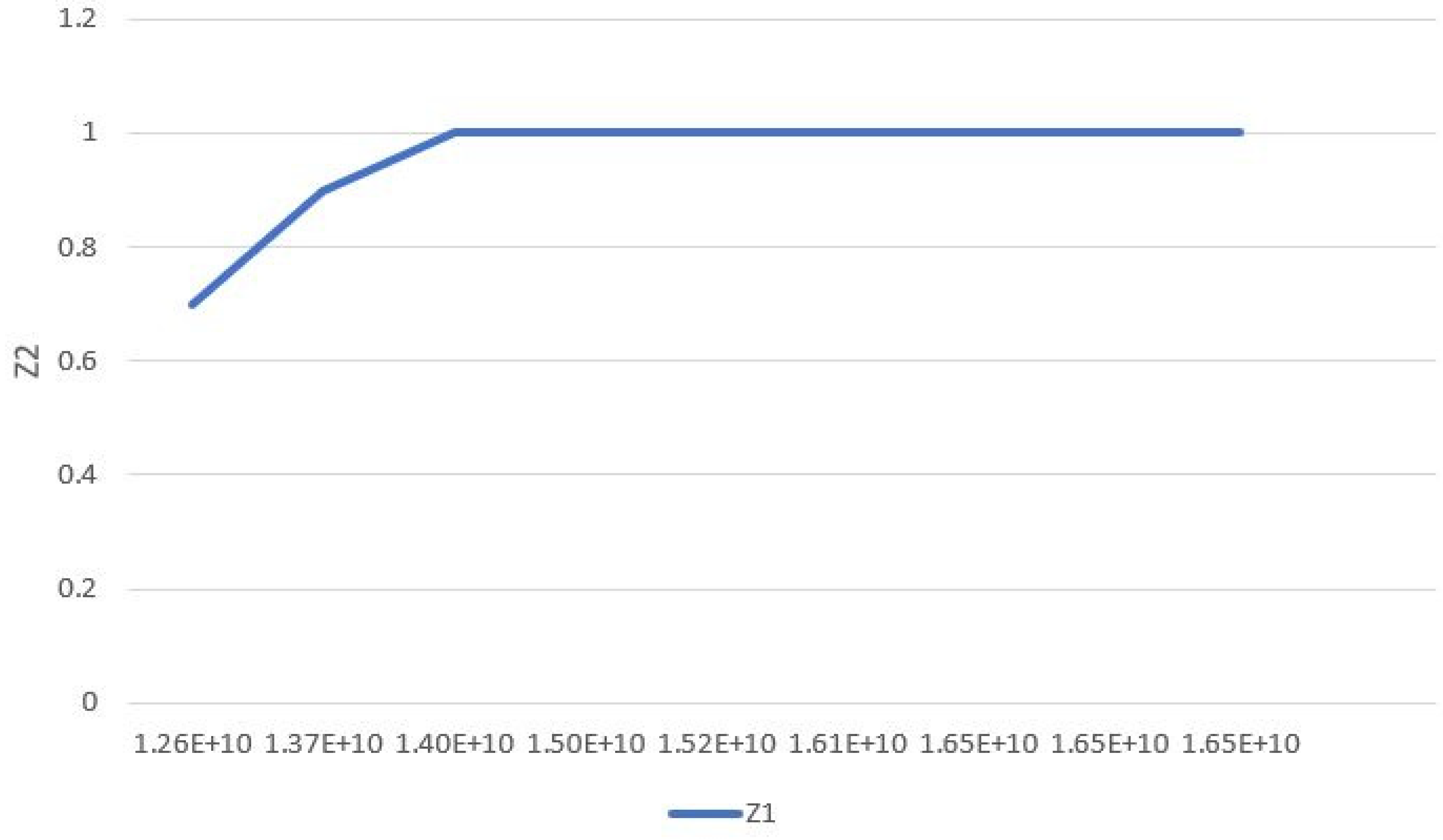
Regarding the two objective functions that are contrary to each other, an increase in the first objective function will lead to a decline in the second objective function. Figure 9 displays the contrast between these two objective functions at β = 0.1.
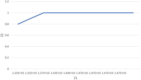
Figure 9.
Representation of the two objective functions in the multi-period model at the minimum satisfaction level of 0.1.
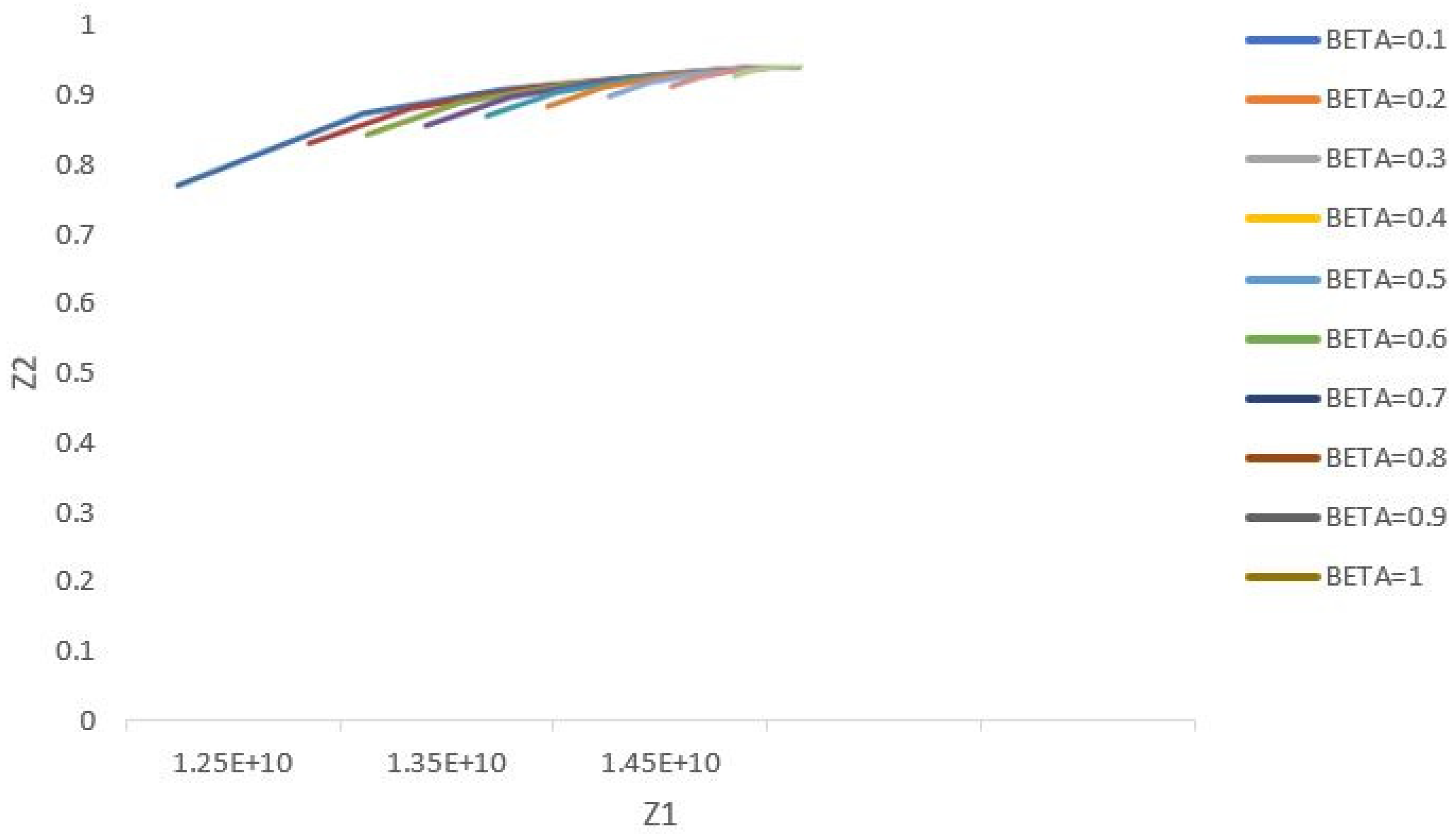
With respect to this point that the above figure has a different shape at different levels of minimum customer satisfaction, Figure 10 depicts the computational results.

Figure 10.
Total costs versus customer satisfaction in the multi-period model per the different values of β.
In accordance with the explanations given until now, calculating the appropriate and optimal value of the two parameters α and β will be a problem. Thus, it is imperative to devise a mechanism in order to optimally select these two parameters by heuristic methods.
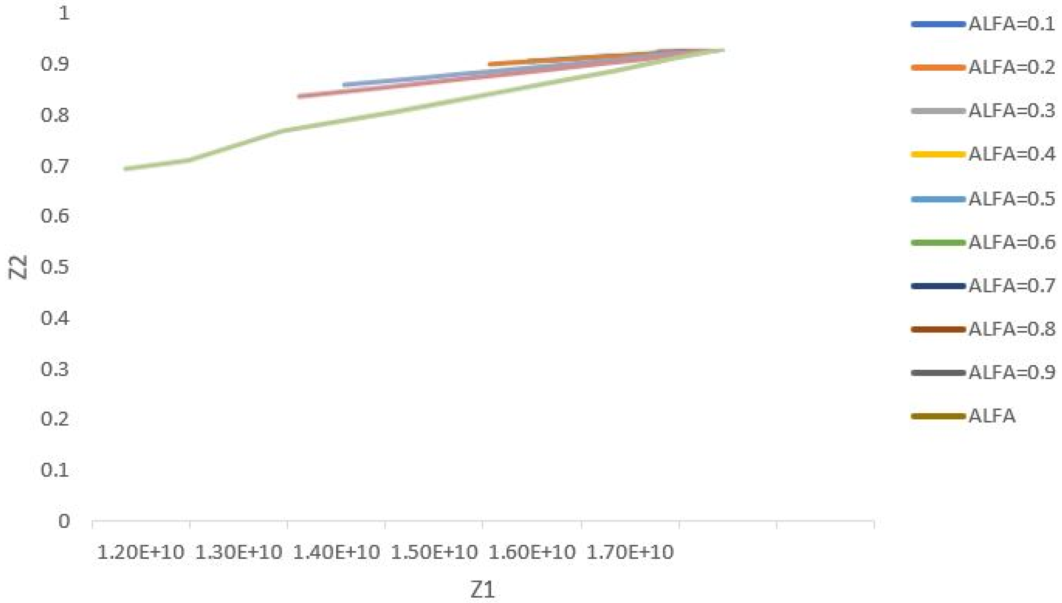
Figure 11 displays the two objective functions’ values for different coefficients of the objective function. The proposed method for measuring the optimal values of the objective functions aims to develop a new function showing customer dissatisfaction as a percentage and the total costs divided by the maximum costs for the different values of α. It is clear that when this new function has the minimum level, it has reached its optimal model. Considering the above graph, it is perceived that the senior management can measure the weighted coefficient of the first objective function by deciding at what minimum percentage they intend to meet the customers’ satisfaction, and accordingly, the other variables and parameters will be determined, too. For example, as a result of selecting β = 0.6, the coefficient of the first objective function (α) is measured as 0.7. Table 6 displays the computational results and the outputs for the abovementioned parameters.
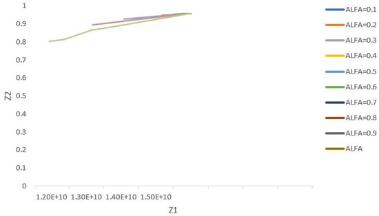
Figure 11.
Total costs versus customer satisfaction in multi-period model per different values of α.

Table 6.
Multi-period model results based on α = 0.7 and β = 0.6.
Table 6 indicates that through adding the inventory management policy to the previous model, as a result of selecting β = 0.6 and the coefficient of the first objective function (α) as 0.7, the minimum cost is equal to 1.42E+10 Iranian Tomans, and the maximum customer satisfaction will equal 94% while both central warehouses have been selected for construction, and out of the eight proposed regional warehouses, only the regional warehouses 1, 3, 4, 6, and 8, i.e., the cities of Isfahan, Khorram-Abad, Rasht, Kerman, and Sari have been selected for construction, respectively.
Basic Model Solution Results along with Green Logistics (Eco-logistics) Policies
To calculate the model’s solution value, it is necessary to simultaneously analyze the two parameters and present the final solution based on the values of these two. These two parameters are the minimum level of meeting the customers’ demands (β) and the first objective function’s weight (α). Table 7 shows the computational results for the different values of these two parameters.

Table 7.
Computational results for green logistics model for different values of α and β.
Considering that the two objective functions are in conflict with each other, the increase in the first objective function will result in a decrease in the second objective function.
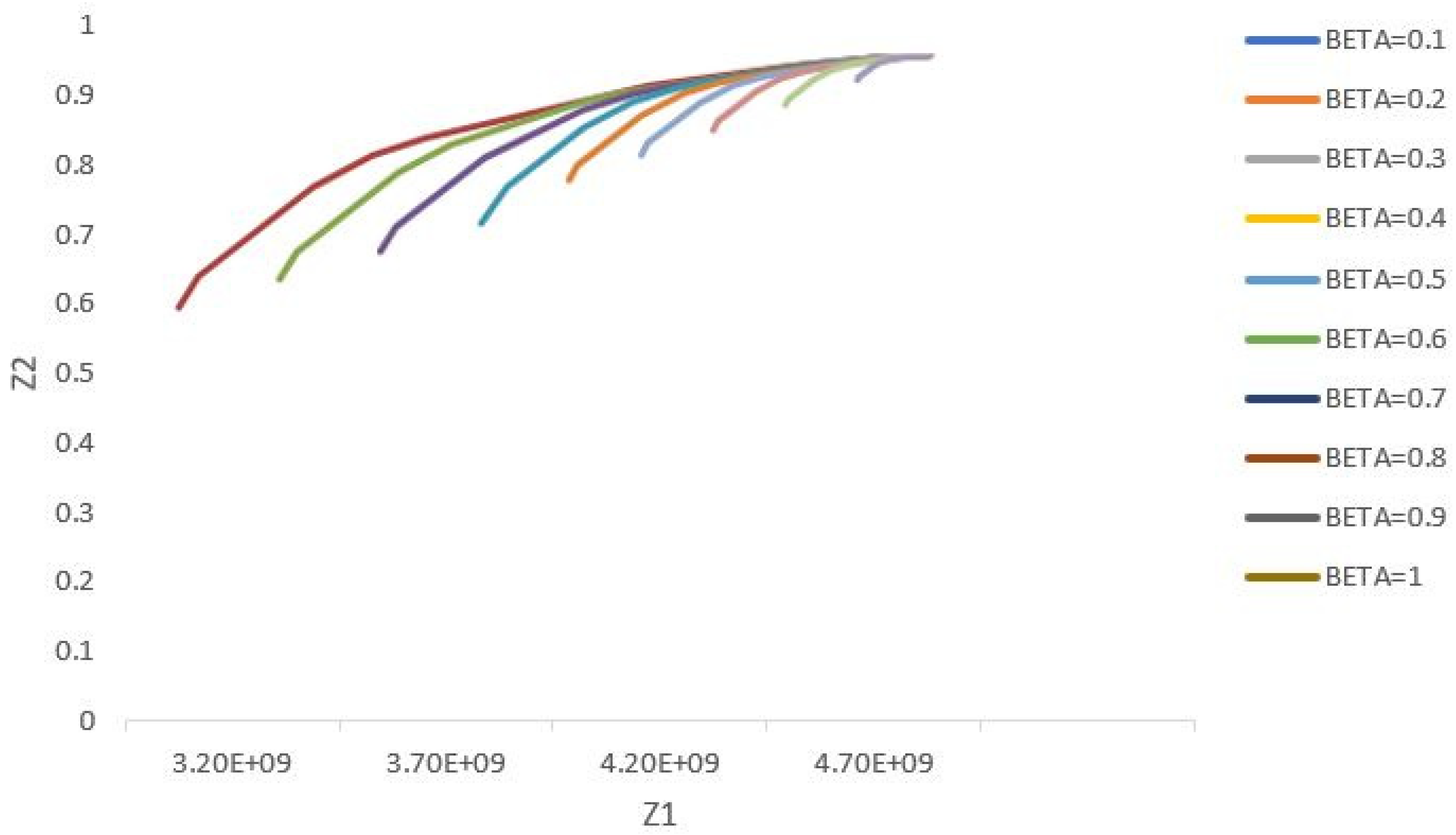
Considering that at different levels of minimum customer satisfaction, Figure 12 has a different shape, the computational results are given in Figure 13.
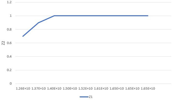
Figure 12.
Representation of two objective functions in green logistics model at minimum satisfaction level of 0.1.
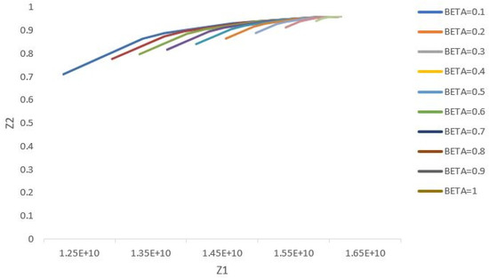
Figure 13.
Total costs versus customer satisfaction in green logistics model for different values of β.
As the explanations given until now indicate, determining the appropriate and optimal value of the two parameters α and β will be a problem. Therefore, it is required to develop a mechanism in order to optimally select these two parameters by heuristic methods.
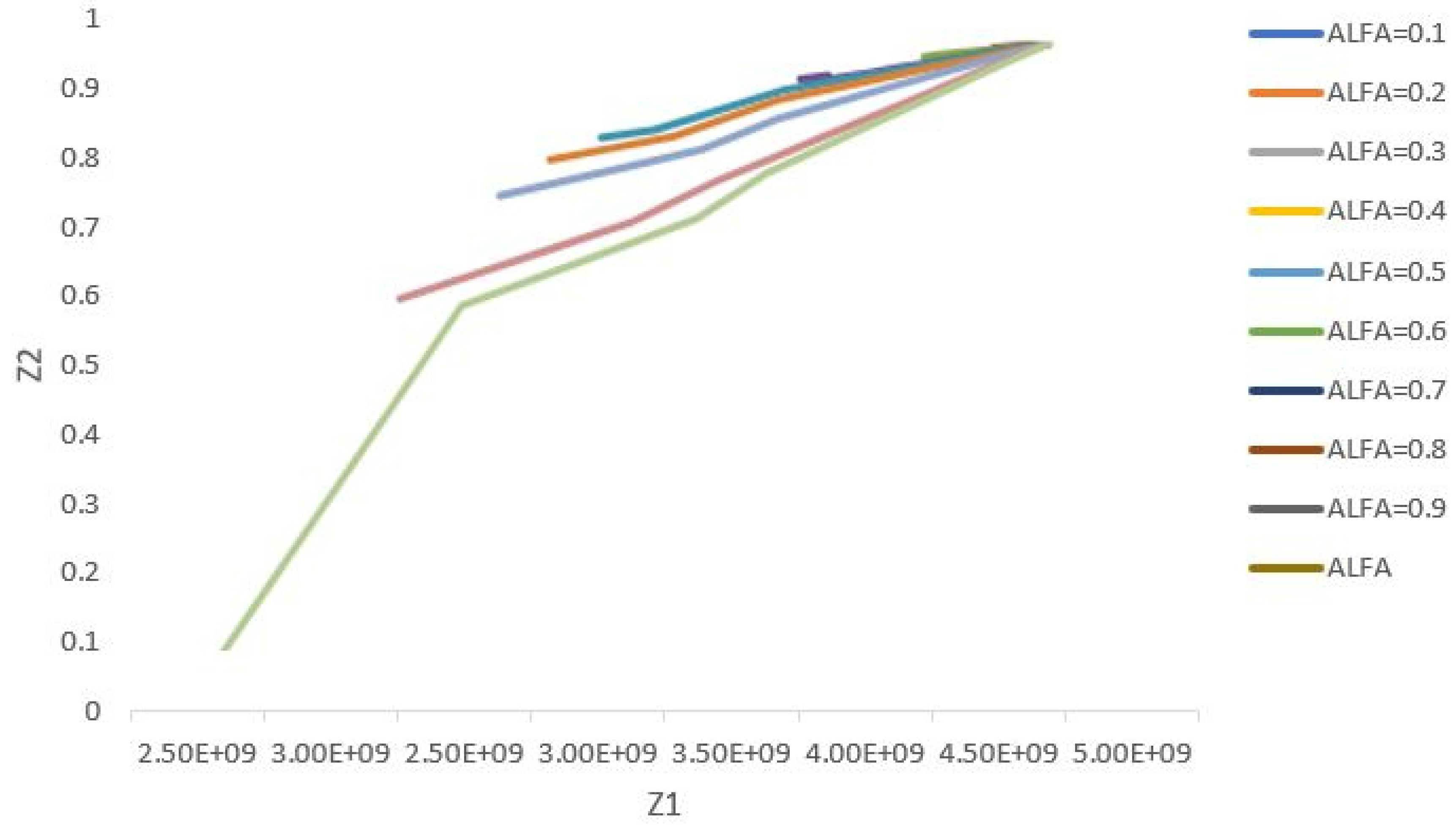
Figure 14 displays the values of the two objective functions for the different coefficients of the objective function. The proposed method for measuring the optimal values of the objective functions targets developing a new function which depicts customer dissatisfaction as a percentage and the total costs divided by the maximum costs for the different values of α. There is no doubt that when this new function has the minimum level, it has reached its optimal model. Considering the above graph, it is concluded that the senior management can measure the weighted coefficient of the first objective function when they decide at what minimum percentage they aim to meet the customers’ satisfaction, and based on this, the other variables and parameters will be determined, too. For instance, as a result of selecting β = 0.6, the coefficient of the first objective function (α) is measured as 0.7. Table 8 shows the computational results and the outputs for the above-stated parameters.
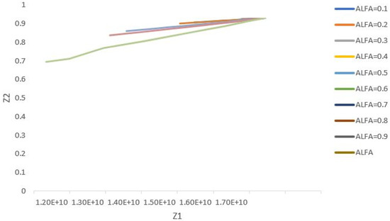
Figure 14.
Total costs versus customer satisfaction in green logistics model for different values of α.

Table 8.
The green logistics model’s results based on α = 0.7 and β = 0.6.
The above table indicates that through adding the inventory management policy to the previous multi-period model, as a result of selecting β = 0.6 and the coefficient of the first objective function (α) as 0.7, the minimum cost is equal to 1.43E+ 10 Iranian Tomans, and the maximum customer satisfaction will equal 96% while both central warehouses have been chosen for construction, and among the eight suggested regional warehouses, only the regional warehouses 1, 3, 4, 6, and 8, i.e., the cities of Isfahan, Khorram-Abad, Rasht, Kerman, and Sari have been picked for construction, respectively.
Framework for Comparing Models’ Outcomes
One of the measures taken in this study was defining and determining the criteria used to measure the performance of different models. According to this and after reviewing similar studies on the performance evaluation criteria, the following indexes have been identified as the measurement criteria. Table 9 includes the summary of the results from analyzing the indices.

Table 9.
Summary of the criteria evaluated in 4 models at optimal levels of α and β.
Pursuant to the results in Table 9 and also to the defined performance evaluation criteria, it is possible to assess the efficiency of the proposed models compared to each other and also in comparison with the condition before the presentation and implementation of the model. Accordingly, we get to compare the criteria separately.
One of the fundamental defined performance criteria is related to customer satisfaction. Figure 15 compares the conditions before and after implementing these four models.
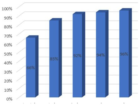
Figure 15.
Comparing the customer satisfaction index before and after implementing the models.
As can be seen, the implementation of the mentioned models tangibly promotes customer satisfaction compared to that before implementing the model. The implementation of the final model has resulted in a 45% increase in customer satisfaction compared to that before the model implementation, a 20% increase compared to the basic model, and a 2.5% increase in the multi-period model’s ratio, which overall has meaningfully improved customer satisfaction.
Another criterion under consideration is the costs of the proposed models. Figure 16 addresses this problem.
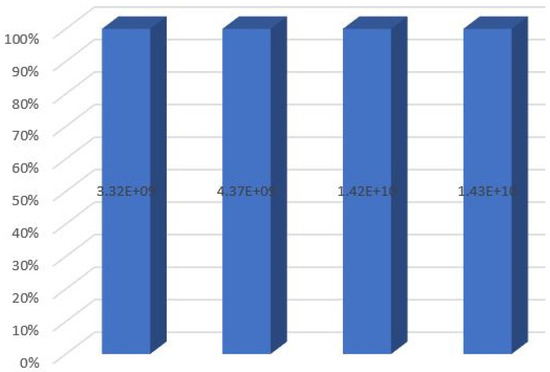
Figure 16.
Comparing the total cost index before and after implementing the model.
As observed in the above figure, the final model implementation only leads to a 0.7% cost increase compared to the multi-period model. Moreover, the tangible cost increase in the single-period model with inventory management policy compared to the multi-period model with inventory is because of considering four time periods in the multi-period model while not considering the construction costs that occur only in one period; the costs in the multi-period model, i.e., four-period model are only 2.7 times more than those of the single-period model with inventory management policy, which means the improvement of the model considering the index of costs.
5. Discussion and Conclusions
The proposed basic model is able to evaluate and select the proper locations for constructing the regional and central warehouses based on experts’ opinions. This model has the potential to add different components to increase the accuracy of decisions. The correct determination of the parameter values made the obtained results be in line with the expert predictions. In other words, the correct determination of the parameters has been effective in the correctness of the outputs. The coverage of all the geographical areas and estimation of the construction cost, maintenance cost, and shortage cost of goods are among the important features of the proposed model. Considering the two objective functions of cost minimization and customer satisfaction maximization concurrently in the proposed model resulted in a suitable interaction between these two objective functions. Employing the weighted method to solve the problem by the two objective functions also provided a more accurate and reliable solution. The contribution suggested for selecting the proper option out of the various model outputs in the interaction between the two parameters as α and β created an appropriate benchmark for optimal decisions. Numerical studies on the other outputs extracted from the interaction between these two parameters also verified the appropriateness of the method.
This multi-product model can assist corporate managers with adopting different policies based on the variety of available products and tracing the results of these policies. Modifying the basic model and adding the concept of inventory management to the basic model significantly increased the customer satisfaction level. This improvement becomes more clear when it is recognized that this modification is of an investment nature and does not require to establish facilities and warehouses, and can be easily implemented in real conditions and in a case study. The cost incurred for executing the inventory management policies versus its revenue is favorable and remarkable, and guarantees its implementation. In this respect, it is required to state that adding inventory management in location decisions is the combination of two strategic and tactical problems in which developing the study period has made it possible to combine these two types of decisions. Modifying the model and adding the potential for inventory management does not exert any tangible effect on the transportation costs from the regional warehouse to the customer, but it increases the transportation costs from the central warehouse to the regional warehouse, the point which indicates the stability of the customer’s behavior and the favorable effect induced by the model modification in the inventory (stock) replenishment of the regional warehouses. On the other hand, a higher potential for inventory management relative to the basic model has boosted the customer satisfaction level according to the separation of the different types of goods and accordingly, it exerts a positive effect. Promoting the power for making decisions and presenting a multi-period model compared with the basic model and the modified one taking the ability for inventory management into account led to increased customer satisfaction with the system. Finally, considering the concept of green logistics and the possibility of returning waste and unused parts simultaneously increased the customer satisfaction level and reduced costs compared to the other models.
At first glance, it seems that adopting this approach meaningfully increased the costs of the system, but in fact, it is not true, and regarding the implementation of four time periods, the aforementioned costs should be considered as a quarter of the mentioned figure. Therefore, paving the ground for multi-period capability reduces system costs. Implementing the multi-period model resulted in an appropriate increase in customer satisfaction through the separation of the product group and led to 100% satisfaction in the three product groups. The implementation of the multi-period model increased customer satisfaction in different warehouses. The implementation of the multi-period model simultaneously had an effect on the costs and their reduction, and the revenue increase resulted in higher profitability for the company.
Suggestions intended to increase the company’s profitability and customer satisfaction level:
Pursuant to the tips and conclusions introduced in the previous section, the following suggestions are presented as the output of the current project investigations:
- Employing a multi-period model along with the power of inventory management so that it leads to reduced costs and increased revenue.
- With respect to the variety of available products, the number of product groups should be increased and included in the proposed model.
- Reducing the time of ordering periods to better use the multi-period model, supplying faster and more up-to-date customer demands in the year, and removing the barriers of the inventory cost increase through modeling and making decisions at the tactical and operational level.
- Raising the number of customers and applying the proposed model to the actual number of customers. It is worth mentioning that in this model, they were integrated into the provincial centers to facilitate the modeling of customer demand.
- Constructing regional warehouses in the locations suggested by the model outputs considering the construction cost and setting up and storing the goods in these warehouses.
- Launching the central warehouse number 2 when its effectiveness gets approved in all the models to properly benefit from it.
- Regularly controlling the proposed performance evaluation indices considering the possibility of changing the supply or demand pattern and making suitable decisions accordingly.
Suggestions for further studies:
As mentioned in the previous sections, the presented basic model is equipped with improvement potential and adds more components to it. Considering the knowledge about the case study environment and the thorough literature review in this research, the following cases are introduced as suggestions and areas for future studies and research cases:
- Investigating the demand pattern in various time periods and the possibility of presenting a supplementary model for the probability mode of demand.
- Investigating the profit from waste recycling.
- Investigating the benefits of the brand’s mental image in terms of compliance with environmental issues.
- Considering production issues in the supply chain and distribution system.
- Including the demand of the different classes of customers in the distribution system and locating facilities; accordingly, in other words, assessing the effect of marketing decisions on the strategic macro-decisions of facility location.
- Considering other location benchmarks.
- Determining the order supply deadline for all sorts of goods orders and programming to supply them within the deadline and its effect on facility location problems.
- Considering other objective functions like social aspects, employment rates, and environmental impacts according to the priorities of managers and decision-makers.
Author Contributions
Conceptualization, M.K., J.A. and D.B.; methodology, M.K., J.A. and D.B.; software, M.K., J.A. and D.B.; validation, M.K., J.A. and D.B.; formal analysis, M.K., J.A. and D.B.; investigation, M.K., J.A. and D.B.; resources, M.K., J.A. and D.B.; data curation, M.K., J.A. and D.B.; writing—original draft preparation, M.K. and D.B.; writing—review and editing, M.K., J.A. and D.B.; visualization, M.K., J.A. and D.B.; supervision, M.K. and J.A.; project administration, M.K., J.A. and D.B. All authors have read and agreed to the published version of the manuscript.
Funding
This research received no external funding.
Data Availability Statement
The original contributions presented in the study are included in the article; further inquiries can be directed to the corresponding authors.
Conflicts of Interest
The authors declare no conflicts of interest.
References
- Kamalahmadi, M.; Parast, M.M. A review of the literature on the principles of enterprise and supply chain resilience: Major findings and directions for future research. Int. J. Prod. Econ. 2016, 171, 116–133. [Google Scholar] [CrossRef]
- Wang, G.; Gunasekaran, A.; Ngai, E.W.T.; Papadopoulos, T. Big data analytics in logistics and supply chain management: Certain investigations for research and applications. Int. J. Prod. Econ. 2016, 176, 98–110. [Google Scholar] [CrossRef]
- Alshubiri, F. The Impact of Green Logistics-Based Activities on the Sustainable Monetary Expansion Indicators of Oman. J. Ind. Eng. Manag. 2017, 10, 389–405. [Google Scholar] [CrossRef]
- Sheikh Azadi, A.H.; Shamsi Nesary, V.; Kebriyaii, O.; Khalilzadeh, M.; Antucheviciene, J. Design of a Green Supply Chain Based on the Kano Model Considering Pricing. Sustainability 2023, 15, 13038. [Google Scholar] [CrossRef]
- Liou, J.J.H.; Tamošaitienė, J.; Zavadskas, E.K.; Tzeng, G.-H. New hybrid COPRAS-G MADM Model for improving and selecting suppliers in green supply chain management. Int. J. Prod. Res. 2015, 54, 114–134. [Google Scholar] [CrossRef]
- Scott, J.; Ho, W.; Dey, P.K.; Talluri, S. A decision support system for supplier selection and order allocation in stochastic, multi-stakeholder and multi-criteria environments. Int. J. Prod. Econ. 2015, 166, 226–237. [Google Scholar] [CrossRef]
- Dweiri, F.; Kumar, S.; Khan, S.A.; Jain, V. Designing an integrated AHP based decision support system for supplier selection in automotive industry. Expert Syst. Appl. 2016, 62, 273–283. [Google Scholar] [CrossRef]
- Mogeni, L.M.; Kiarie, D.M. Effect of Green Logistics Practices on Performance of Supply Chains in Multinational Organizations in Kenya. Ind. Eng. Lett. 2016, 6, 40–50. [Google Scholar]
- Muangpan, T.; Chaowarat, M.; Neamvonk, J. The key activities of green logistics management in the Thai automotive industry. J. Arts Sci. Commer. 2016, 7, 1–11. [Google Scholar] [CrossRef]
- Brusset, X.; Teller, C. Supply chain capabilities, risks, and resilience. Int. J. Prod. Econ. 2017, 184, 59–68. [Google Scholar] [CrossRef]
- Ribeiro, J.P.; Barbosa-Povoa, A. Supply Chain Resilience: Definitions and quantitative modelling approaches. Comput. Ind. Eng. 2018, 115, 109–122. [Google Scholar] [CrossRef]
- Heidari, A.; Imani, D.M.; Khalilzadeh, M. A hub location model in the sustainable supply chain considering customer segmentation. J. Eng. Des. Technol. 2021, 19, 1387–1420. [Google Scholar] [CrossRef]
- Eydi, A.; Fazayeli, S.; Ghafouri, H. Multi-period configuration of forward and reverse integrated supply chain networks through transport mode. Sci. Iran. 2020, 27, 935–955. [Google Scholar] [CrossRef]
- Antucheviciene, J.; Jafarnejad, A.; Amoozad Mahdiraji, H.; Razavi Hajiagha, S.H.; Kargar, A. Robust Multi-Objective Sustainable Reverse Supply Chain Planning: An Application in the Steel Industry. Symmetry 2020, 12, 594. [Google Scholar] [CrossRef]
- Gholamian, N.; Mahdavi, I.; Mahdavi-Amiri, N.; Tavakkoli-Moghaddam, R. Hybridization of an interactive fuzzy methodology with a lexicographic min-max approach for optimizing a multi-period multi-product multi-echelon sustainable closed-loop supply chain network. Comput. Ind. Eng. 2021, 158, 107282. [Google Scholar] [CrossRef]
- Alinezhad, M.; Mahdavi, I.; Hematian, M. A fuzzy multi-objective optimization model for sustainable closed-loop supply chain network design in food industries. Environ. Dev. Sustain. 2022, 24, 8779–8806. [Google Scholar] [CrossRef]
- Pazhani, S.; Mendoza, A.; Nambirajan, R.; Narendran, T.T.; Ganesh, K.; Olivares-Benitez, E. Multi-period multi-product closed loop supply chain network design: A relaxation approach. Comput. Ind. Eng. 2021, 155, 107191. [Google Scholar] [CrossRef]
- Nazari-Ghanbarloo, V.; Ghodratnama, A. Optimizing a robust tri-objective multi-period reliable supply chain network considering queuing system and operational and disruption risks. Oper. Res. 2021, 21, 1963–2020. [Google Scholar] [CrossRef]
- Rabe, M.; Gonzalez-Feliu, J.; Chicaiza-Vaca, J.; Tordecilla, R.D. Simulation-Optimization Approach for Multi-Period Facility Location Problems with Forecasted and Random Demands in a Last-Mile Logistics Application. Algorithms 2021, 14, 41. [Google Scholar] [CrossRef]
- Zarrat Dakhely Parast, Z.; Haleh, H.; Avakh Darestani, S. Green reverse supply chain network design considering location-routing-inventory decisions with simultaneous pickup and delivery. Environ. Sci. Pollut. Res. 2021. [Google Scholar] [CrossRef]
- Abdolazimi, O.; Bahrami, F.; Shishebori, D. A multi-objective closed-loop supply chain network design problem under parameter uncertainty: Comparison of exact methods. Environ. Dev. Sustain. 2022, 24, 10768–10802. [Google Scholar] [CrossRef]
- Maliki, F.; Souier, M.; Dahane, M. A multi-objective optimization model for a multi-period mobile facility location problem with environmental and disruption considerations. Ann. Oper. Res. 2022, 1–26. [Google Scholar] [CrossRef] [PubMed]
- Gupta, S.; Vijaygargy, L.; Sarkar, B. A bi-objective integrated transportation and inventory management under a supply chain network considering multiple distribution networks. RAIRO Oper. Res. 2022, 56, 3991–4022. [Google Scholar] [CrossRef]
- Bortolini, M.; Calabrese, F.; Gabriele Galizia, F.; Mora, C. A three-objective optimization model for mid-term sustainable supply chain network design. Comput. Ind. Eng. 2022, 168, 108131. [Google Scholar] [CrossRef]
- Mogale, D.G.; De, A.; Ghadge, A.; Aktas, E. Multi-objective modelling of sustainable closed-loop supply chain network with price-sensitive demand and consumer’s incentives. Comput. Ind. Eng. 2022, 168, 108105. [Google Scholar] [CrossRef]
- Al-Refaie, A.; Kokash, T. Optimization of sustainable reverse logistics network with multi-objectives under uncertainty. J. Remanuf. 2023, 13, 1–23. [Google Scholar] [CrossRef]
- Meidute-Kavaliauskiene, I.; Yıldırım, F.; Ghorbani, S.; Činčikaitė, R. The Design of a Multi-Period and Multi-Echelon Perishable Goods Supply Network under Uncertainty. Sustainability 2022, 14, 2472. [Google Scholar] [CrossRef]
- Allehashemi, T.; Hassanzadeh Amin, S.; Zolfaghari, S. A proposed multi-objective model for cellphone closed-loop supply chain optimization based on fuzzy QFD. Expert Syst. Appl. 2022, 210, 118577. [Google Scholar] [CrossRef]
- Abdi, F.; Farughi, H.; Sadeghi, H.; Arkat, J. Location-inventory-reliability optimisation problem in a multi-objective multi-period three-level supply chain network with stochastic demand. Eur. J. Ind. Eng. 2023, 17, 479–528. [Google Scholar] [CrossRef]
- Arab Momeni, M.; Jain, V.; Bagheri, M. A Multi-Objective Model for Designing a Sustainable Closed-Loop Supply Chain Logistics Network. Logistics 2024, 8, 29. [Google Scholar] [CrossRef]
- Varshney, N.; Gupta, S.; Ahmed, A. Addressing uncertainty in closed-loop supply chain networks: A multi-objective approach to integrated production and transportation problems. J. Model. Manag. 2024, in press. [Google Scholar] [CrossRef]
- Xia, H.; Chen, Z.; Milisavljevic-Syed, J.; Salonitis, K. Uncertain programming model for designing multi-objective reverse logistics networks. Clean. Logist. Supply Chain 2024, 11, 100155. [Google Scholar] [CrossRef]
Disclaimer/Publisher’s Note: The statements, opinions and data contained in all publications are solely those of the individual author(s) and contributor(s) and not of MDPI and/or the editor(s). MDPI and/or the editor(s) disclaim responsibility for any injury to people or property resulting from any ideas, methods, instructions or products referred to in the content. |
© 2024 by the authors. Licensee MDPI, Basel, Switzerland. This article is an open access article distributed under the terms and conditions of the Creative Commons Attribution (CC BY) license (https://creativecommons.org/licenses/by/4.0/).

