Article

Emission Control in Expressway Systems: Vehicle Emission Inventory and Policy Scenario Analysis

School of Transportation, Southeast University, Nanjing 210096, China
*
Author to whom correspondence should be addressed.
Systems 2024, 12(8), 273; https://doi.org/10.3390/systems12080273
Submission received: 25 June 2024 / Revised: 26 July 2024 / Accepted: 27 July 2024 / Published: 29 July 2024

Abstract

:
Expressway systems play a vital role in facilitating intercity travels for both passengers and freights, which are also a significant source of vehicle emissions within the transportation sector. This study investigates vehicle emissions from expressway systems using the COPERT model to develop multi-year emission inventories for different pollutants, covering the past and future trends from 2005 to 2030. Thereinto, an integrated SARIMA-SVR method is designed to portray the temporal variation of vehicle population, and the possible future trends of expressway vehicle emissions are predicted through policy scenario analysis. The Jiang–Zhe–Hu Region of China is taken as the case study to analyze emission control in expressway systems. The results indicate that (1) carbon monoxide (CO) and volatile organic compounds (VOCs) present a general upward trend primarily originating from passenger vehicles, while nitrogen oxides (NOx) and inhalable particles (PM) display a slowing upward trend with fluctuations mainly sourcing from freight vehicles; (2) vehicle population constraint is an effective emission control policy, but upgrading the medium- and long-haul transportation structure is necessary to meet the continuous growth of intercity trips. Expressway vehicle emission reduction effectiveness can be further enhanced by curtailing the update frequency of emission standards, along with the scrapping of high-emission vehicles.

1. Introduction

The continuous economic development and urbanization in the past two decades have stimulated the prosperity of China’s auto industry, and vehicle population (VP) in China has reached 417 million in 2022 [1]. Traffic-related emissions have grown to be one of the main anthropogenic contributors to atmospheric pollution that simultaneously influence air quality and human health [2,3]. For example, the vehicle emissions of nitrogen oxides (NOx) and volatile organic compounds (VOCs) are recognized as significant precursors of photochemical smog by production photochemical oxidizing substances (e.g., ozone), whilst particulate matter (PM) and carbon monoxide (CO) emitted from vehicles may enter and damage lung and bronchus, causing long-term health effects [4]. Accordingly, four pollutants from the transportation sector account for 35.0%, 16.8%, 6.6%, and 18.5% of the total NOx, VOCs, PM, and CO emissions, respectively, in China in 2017 [5]. Considering the rapid growth of VP and associated negative implications, various vehicle emission control policies (e.g., updating vehicle emission standards) have been developed successively in China. Yet, these policies have long-term impacts on vehicle emissions. Therefore, it is of great necessity to establish multi-year vehicle emission inventories, and analyze the vehicle emission trends and characteristics from a long-term perspective.
On-road vehicle emissions can be further split into intracity emissions and intercity emissions [6]. The former involves a hierarchy of roads (e.g., major arterials, minor arterials, collectors) that are typically used for intracity trips in the urban areas of one city/county, while the latter mainly relies on the national and provincial-level expressways for intercity trips between cities/counties. The expressway systems are considered as a crucial catalyst for the integrated development of urban agglomerations, with the primary function serving intercity passenger travels and freight mobilities. Meanwhile, most intercity trips are medium and long haul, and the penetration rate of new energy vehicles on expressways at present is quite low due to range anxiety. Thereby, the majority of vehicles using expressway systems are still conventional fuel vehicles in the short term, which are different from the tendency of intracity trips. Because of the expressways’ particularity, it is valuable to develop dedicated long-term vehicle emission inventories emitted from expressway systems. Especially for China, it has the largest expressway network over the world, with a total length of 169,100 km as of 2021 [7].
The Jiang–Zhe–Hu (JZH) region is composed of two provinces (Jiangsu and Zhejiang) and one municipality (Shanghai) in eastern coastal China. It plays a leading role in the demographic, economic, and technological development of China [8]. At the same time, it has a well-developed expressway system, with a density of 505.6 km per million square kilometers by 2021 [9]. For freight transport, most goods with an origin and destination in the JZH region can be delivered to customers within one day [10]. The expressway toll system (ETS) records detailed vehicle amounts and vehicle kilometers traveled when vehicles enter and exit ETS between two different toll gates. It provides a data basis to obtain the historical trends of vehicle emissions emitted from expressways. Nevertheless, expressway vehicle emission-related studies in the JZH region are limited, possibly due to the data availability of the ETS dataset. In addition, the long-term influence mechanism of vehicle population growth and increasingly stringent emission standards on expressway vehicle emissions is complicated. However, mechanism analysis, future trend prediction, and scenario simulation of expressway vehicle emissions in the JZH region are not comprehensively studied.
In view of above analysis, the main contributions of this study are as follows: (1) The Computer Programme to Calculate Emissions from Road Transport (COPERT) model is utilized to develop the multi-year vehicle emission inventories of expressway systems in the JZH region, covering the past and future trends from 2005 to 2030. (2) Based on the level of different policy environments, nine scenarios are set up. A Seasonal Autoregressive Integrated Moving Average (SARIMA) model enhanced by Support Vector Regression (SVR) is built to capture the mechanism behind the temporal variation of VP and further predict the possible future evolution trends of expressway vehicle emissions under various scenarios. Studying the characteristics of expressway vehicle emissions in the JZH region provides beneficial suggestions and references for environmental policy formulation and the sustainable development of expressway systems in other similar regions.
The outline for this paper is organized as follows. Section 2 summarizes the extant literature on vehicle emissions. Section 3 describes data and research methodology. Section 4 presents results and discussions. Finally, conclusions are drawn in Section 5.

2. Literature Review

Vehicle emission inventory is essential for understanding vehicle pollution and evaluating various policy options [3,11]. According to the temporal granularity of available data, it can be divided into two categories: long-term inventory and short-term inventory. In this study, we concentrate the review of literature on relevant studies in the first category.
Long-term vehicle emission inventory typically uses months or even years as the unit to describe the past and future trends of vehicle emissions at the national or localized levels. The measurement of vehicle emissions contains two methods: the top–down method and the bottom–up method [12,13]. The former is based on traffic energy consumption and energy conversion factors, while the latter is based on vehicle population, vehicle kilometers traveled, and emission factors. Furthermore, by and large, the emission inventory of air pollutants from mobile sources can be estimated by means of on-road vehicle emission models, such as Mobile Source Emissions Factor (MOBILE), Motor Vehicle Emission Simulator (MOVES), International Vehicle Emission (IVE), and Computer Programme to Calculate Emissions from Road Transport (COPERT). Among them, due to similarities between vehicle manufacturing technologies and emission regulations in China and many European countries, the COPERT model proposed by the European Union has been widely applied to calculate the vehicle emissions in different regions of China [14,15,16].
Based on the above vehicle emission models, a number of vehicle emission inventories have been conducted in developed countries, such as the United States and Europe [17,18,19,20,21]. In contrast, research on vehicle emission inventories started late in China but has quickly progressed. Some scholars developed the multi-year vehicle emission inventories on the national basis of China for different air pollutants [22,23,24,25,26]. In recent years, numerous studies have paid more attention to regional and city-level vehicle emissions. For example, regions such as the Beijing–Tianjin–Hebei region [27,28,29] and Harbin–Changchun Megalopolis [30]; provinces such as Guangdong [31], Shandong [32], Inner Mongolia [4], and Yunnan [33]; cities such as Beijing [34,35], Tianjin [36], and Langfang [37]. Furthermore, some studies also investigated future vehicle emissions to evaluate the effects of various emission policies using scenario analysis [28,34,35,36].
The JZH region is the core of the Yangtze River Delta (YRD), which is one of the fastest growing and richest urban agglomerations in China. The multi-year vehicle emission inventories of YRD from 1999 to 2015 were calculated for different air pollutants using the COPERT model, and various policy options were assessed [15,38]. Results suggest that the updates of stringent emission standards be more frequent. Previous studies have provided abundant paradigms for establishing the long-term emission inventories of road transport and useful references for vehicle emission reduction policies. However, research specifically for long-term vehicle emission inventories emitted from expressway systems appears to be scarce. Expressway systems undertake the bulk of intercity trips, the function of which is significantly different from other road types for intracity trips. Due to the expressways’ particularity, it is worthwhile to establish dedicated emission inventories. Nevertheless, the data conditions in the existing studies are insufficient, while the expressway toll system (ETS) dataset can provide high-quality traffic data information to accurately characterize expressway vehicle emissions.
Furthermore, different vehicle emission control policies (e.g., updating vehicle emission standards) have been successively implemented during the past two decades. The implicit impact of these policies may increase the complexity and uncertainty of predicting the future evolution trend of expressway vehicle emissions, which is primarily reflected in the temporal variation of VP for different types of vehicles. Fortunately, the application of machine learning methods is capable of capturing the influencing mechanism of policies behind the temporal variation of VP. Instead of using the single SARIMA method, this study employs the integrated SARIMA-SVR approach, which has proven successful in forecasting statistical indicators within the aviation industry [39]. It can improve the forecast performance and describe the nonlinear mapping relationship that exists in the inter-monthly VP data. Moreover, with the different levels of various policy options considered, a set of scenarios are generated to fully explore the possible future changes of expressway vehicle emissions in the JZH region, which is particularly instrumental for decision makers to comprehensively understand the effects of vehicle emission control and accumulate experience for seeking the sustainable development of expressway systems in similar regions.

3. Data and Method

3.1. Study Area and Data Sources

The Jiang–Zhe–Hu (JZH) region is located in eastern coastal China, covering a total area of 219 thousand square kilometers. It is one of the most active, open, and innovative regions in China in terms of the demographic, economic, and technological development. In 2021, the resident population reached 175.3 million, and the total annual GDP attained CNY 23,309.5 billion. Meanwhile, the expressway system of the JZH region is extensively developed, and its total length amounted to 11,074 km as of 2021 [40]. The expressway network of the JZH region is depicted in Figure 1.
Data utilized in this study have two main sources. The first data source is collected from the expressway toll system of the JZH region, dubbed the JZH-ETS dataset. In practice, each expressway in China has a set of mileposts, and any two contiguous mileposts constitute a road segment with fixed kilometers. Expressway trips are recorded when vehicles enter and exit two different expressway toll gates. For each trip, the travel path is composed of several road segments between two toll gates according to the shortest travel distance using the expressway service. The JZH-ETS dataset involves the aggregate traffic data information of monthly vehicle population (VP) of all the road segments in the JZH expressway network for various vehicle types during the period 2005–2020, which is utilized to obtain multi-year expressway vehicle emission inventories. The second data source is collected from the national and localized statistical yearbooks, including the National Bureau of Statistics of China (NBSC), Jiangsu Bureau of Statistics (JBS), Zhejiang Bureau of Statistics (ZBS), and Shanghai Bureau of Statistics (SBS).

3.2. Expressway Vehicle Emission Calculation

In this study, the multi-year vehicle emission inventories of the expressway system in the JZH region are calculated by using the COPERT model. Expressway vehicle emissions of pollutants are associated with vehicle population (VP), vehicle kilometers travelled (VKT), and emission factors (EF). The calculated formula is expressed as:
E i , y , n = j h k V P i , j , h , k , y · V K T k · E F i , j , h , n
where E i , y , n is the amount of pollutant n from vehicle type i emitted at the time of year y . V P i , j , h , k , y represents the vehicle population of vehicle type i with fuel type h under emission standard j traversing road segment k at the year of y . V K T k represents the travel distance traversing road segment k . E F i , j , h , n represents the emission factor for pollutant type n of vehicle type i with fuel type h under the emission standard j . In the expressway system, there are eight vehicle types including small-duty passenger vehicle (SDV), medium-duty passenger vehicle (MDV), heavy-duty passenger vehicle (HDV), small-duty truck (SDT), medium-duty truck (MDT), heavy-duty truck (HDT), extra-large truck, and container truck. Fuel types include gasoline and diesel. Vehicle emission standards contain pre-China I, China I, China II, China III, China IV, China V, and China VI. Pollutants analyzed in this study include nitrogen oxides (NOx), volatile organic compounds (VOCs), particulate matter (PM), and carbon monoxide (CO).
The JZH-ETS dataset records in detail the monthly VP of all vehicle types for all expressway road segments in the JZH region. Let V P i , k , y denote the vehicle population of vehicle type i traversing road segment k during year y . In China, when one new vehicle emission standard is enacted, newly registered vehicles should follow such standard and meantime vehicles reaching a regulated age or mileage should be scrapped [41]. Then, the population of newly registered vehicles and survival-rate curves resulting from vehicle scrappage are essential for acquiring vehicle age distribution of V P i , k , y that impacts the term V P i , j , k , y in Equation (1). In this section, the survival-rate curves of different vehicle types are based on previous studies [33,41,42,43]. V P i , j , k , y is calculated by the following equations:
V R i , a , y = N i , y a × R i , a
V R i , y = a V R i , a , y
X i , a , y = V R i , a , y V R i , y
V P i , j , k , y = a γ y a , j X i , a , y V P i , k , y
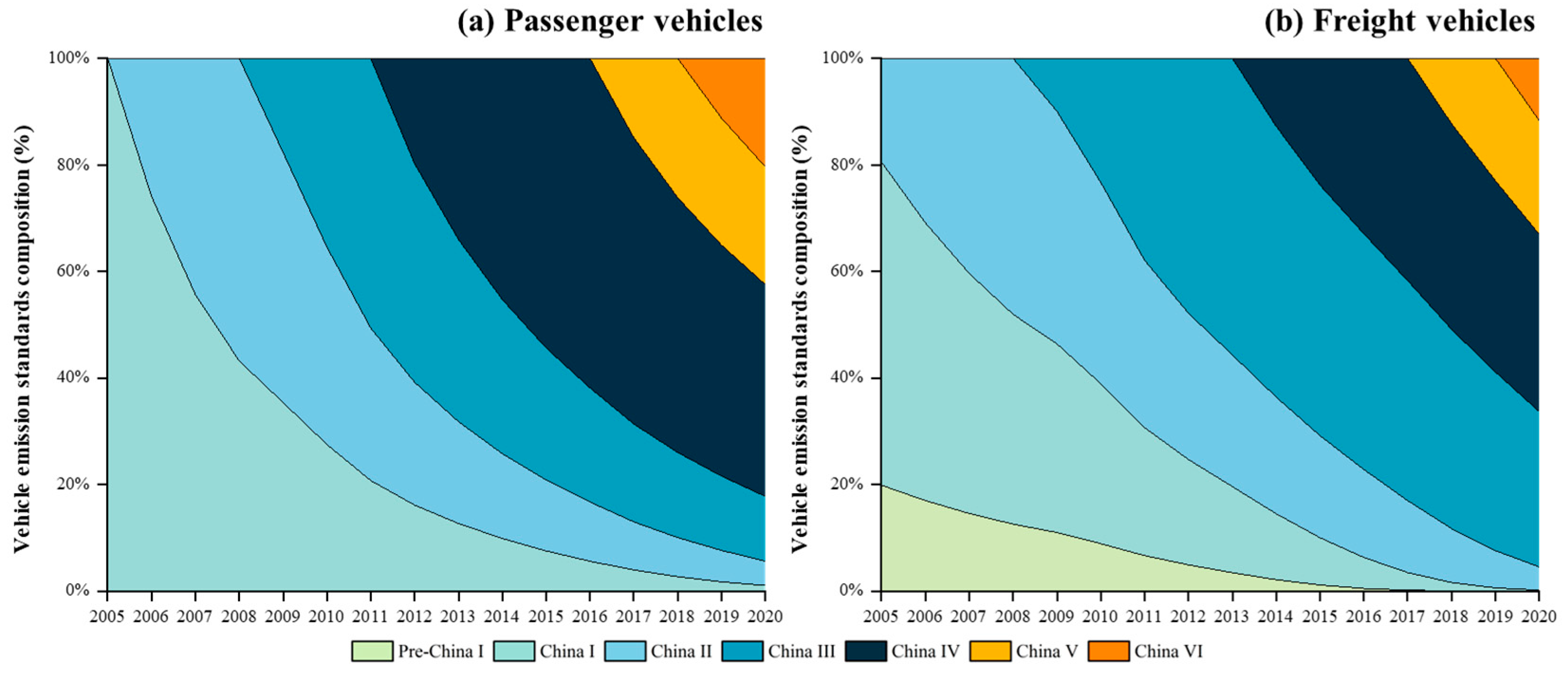
where V R i , a , y is the vehicle population of vehicle type i with age a at the year of y . N i , y a is the number of newly registered vehicles for vehicle type i in year y a , which is from the statistical yearbooks of the JZH region. R i , a is the survival rate for vehicle type i with age a . V R i , y denotes vehicle population of vehicle type i at the year of y . As an indicator of vehicle age distribution, X i , a , y denotes the percentage of vehicles with age a for vehicle type i in year   y . γ y a , j is a binary parameter which equals 1 if the newly registered vehicles obey emission standard j in year y a , and 0 otherwise. Meanwhile, γ y a , j = 1 always holds. On this basis, the compositions of VP with various emission standards for passenger vehicles and freight vehicles, respectively, from 2005 to 2020, are displayed in Figure 2.
In addition to emission standards, the other parameters such as average vehicle speed, meteorological conditions are also needed in the COPERT model, and the model parameters primarily contain average speed, Reid vapor pressure (RVP), relative humidity (RH), and temperature. The values of parameters follow the extant literatures such as Cai and Xie [14], Yao and Song [44], Sun et al. [36], and Zhao [45], and monthly meteorological parameters are derived from the Meteorological Data Sharing System of China.

3.3. Forecasting Model of Vehicle Population

Equation (1) indicates that the calculation of expressway vehicle emissions is contingent on vehicle population (VP), vehicle kilometers travelled (VKT), and emission factors (EF). VKT is known for each road segment between two contiguous mileposts within the expressway system, while EF hinges on the enactment of vehicle emission standards. Then, the VP of different vehicle types becomes the primary uncertain factor that dictates the long-term variation tendency of expressway vehicle emissions.
In the past two decades, various vehicle emission control policies (e.g., increasingly stringent emission standards) have been progressively enacted. These policies implicitly incur the complexity and uncertainty of accurately forecasting future vehicle population using the expressway service, which is mainly reflected in the monthly VP growth for different vehicle types. To capture the influencing mechanism behind the temporal variation of VP, a Seasonal Autoregressive Integrated Moving Average (SARIMA) model enhanced by Support Vector Regression (SVR), dubbed the integrated SARIMA-SVR method, is employed to reveal the nonlinear mapping relationship that exists in the inter-monthly VP data.
The fundamental form of the general SARIMA model is expressed as:
ϕ p B Φ p B m d m D P t = θ q B Θ Q B m ε t
where P t is the non-stationary time series. d and m D are the differences used to remove the seasonality and trend, respectively. B m is the back-shift operator. Φ p B m and ϕ p B are the autoregressive polynomial with seasonal and trend components, while Θ Q B m and θ q B are the moving average polynomial with seasonal and trend components. The residual error ε t is the Gaussian white noise with zero mean and finite variance σ 2 , which is employed in the SVR module.
The general expression of the SVR module is given by:
f x = ω ψ x + b
where ψ x is the kernel function that transforms the input vector ψ x into a high dimensional space with the weight vector ω .
The SARIMA model is adept at isolating linear information from the data, while the SVR module excels in extracting nonlinear information. Therefore, to further enhance the fitting performance, including the applicability and accuracy of the forecasting model, this study utilizes a cascaded ensemble model for monthly VP prediction. First, Equation (6) is applied to calculate the fitted linear sequence P t ^ , and the residual sequence R t represents the sequence of residual errors ε t . The residual sequence R t is then used as input for training and forecasting in the SVR module, expressed as below:
f R t = ω ψ R t + b
where, in our preliminary analysis, different kernel functions are examined and the radial basis kernel function (RBF) is ultimately selected as ψ R t .
By summing the fitted linear sequence P t ^ obtained from the SARIMA model, and the residual fitted sequence R t ^ obtained from the SVR module, the prediction results of the integrated SARIMA-SVR model are derived, as illustrated in Equation (9):
V P t ^ = P t ^ + R t ^
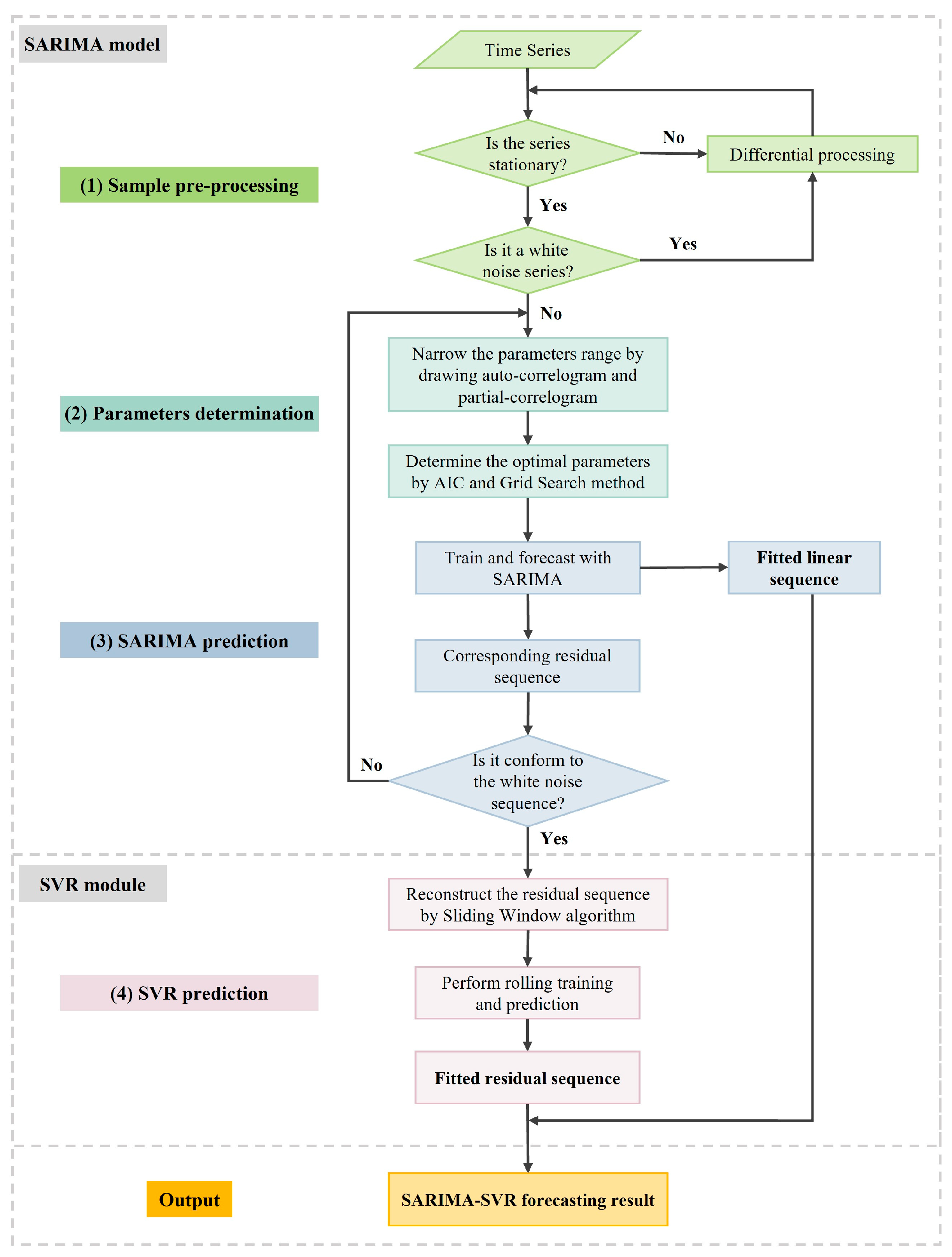
Figure 3 depicts the flowchart of the SARIMA-SVR integrated method, and the associated procedures are described as follows. Readers can refer to Nobre et al. [46], Xu et al. [39], and the references therein for further details.
Step 1. Sample pre-processing: The monthly VP of different vehicle types is first input as the original time series. The prerequisites for creating a SARIMA model are the absence of stationarity and seasonality of the time series. The Augmented Dickey–Fuller (ADF) test is used to ascertain whether the time series is stationary. The trend can be eliminated using differencing if the time series is non-stationary. Additionally, the differenced sequence is also examined through the ADF test to determine whether it exhibits the characteristics of non-white noise. If the sequence represents a white noise series, it indicates a lack of interdependence among the values in the time series, rendering it unsuitable for analysis and necessitating further differencing.
Step 2. Parameter determination: Whereafter, auto-correlogram and partial-correlogram are drawn to narrow the parameters range. Then, use the Akaike Information Criterion (AIC) and Grid Search method to determine the optimal parameters for the S A R I M A ( p , d , q ) × ( P , D , Q ) m model.
Step 3. SARIMA prediction: Train the SARIMA model with the stationary time series training set and use its prediction function to forecast the time series, resulting in the fitted linear sequence P t ^ and the corresponding nonlinear residual sequence R t . Moreover, examine whether the residual sequence exhibits the characteristics of white noise. If the residuals do not conform to the white noise sequence, it indicates the inadequate extraction of the linear component, and necessitates the reestablishment of the model. Otherwise, if the residual sequence fits the white noise characteristics, then move on to Step 4.
Step 4. SVR prediction: Reconstruct R t as a sequence of order u by the Sliding Window Algorithm, and use the SVR model to perform rolling training and prediction on the residual sequence to obtain the fitted residual sequence R t ^ .
Output: The summation of the SARIMA fitted sequence P t ^ and the SVR fitted residual sequence R t ^ yields the predicted V P t ^ of various vehicle types through the utilization of the integrated SARIMA-SVR method.

3.4. Research Framework

In this study, the research framework subsumes three stages, as shown in Figure 4. The first stage is to obtain the multi-year expressway vehicle emission inventories of the JZH region using the COPERT model. The second stage is to forecast the monthly VP variation of different vehicle types by the integrated SARIMA-SVR method. In the third stage, the possible future evolution trends of expressway vehicle emissions are predicted through scenario analysis. Then, expressway vehicle emission reduction policies in the JZH region can be formulated based upon the analysis results.

4. Results and Discussions

4.1. Expressway Vehicle Emission Inventories

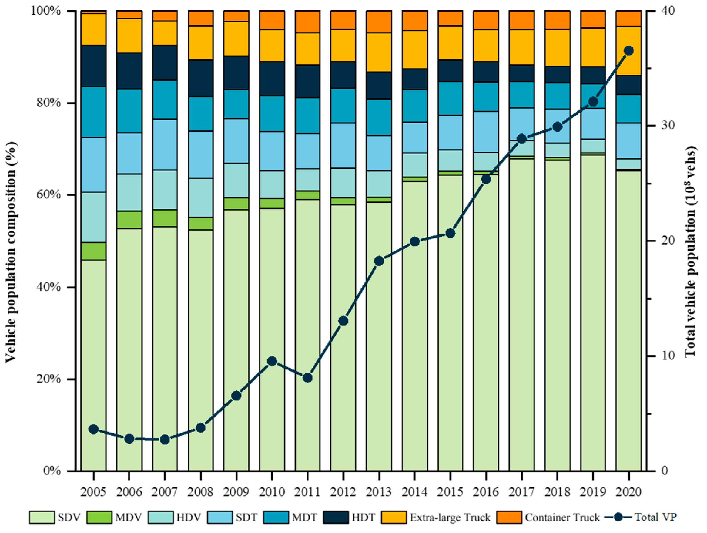
The JZH-ETS dataset includes the monthly VP information of three passenger vehicle types (SDV, MDV, and HDV) and five freight vehicle types (SDT, MDT, HDT, extra-large truck, and container truck). Figure 5 depicts the temporal variation in expressway vehicle population and the associated percentage of different vehicle types in the JZH region from 2005 to 2020. By and large, the vehicle population using the expressway system in the JZH region has shown an upward trend over time with some minor fluctuations. The VP amount increases from 365.1 million in 2005 to 3654.5 million in 2020.
In terms of passenger vehicles, SDV has consistently constituted the main component of the passenger vehicle fleet. Over the past 15 years, there has been a continuous upward trend, with the proportion of SDV in the passenger vehicle fleet steadily increasing from 75.7% in 2005 to 96.1% in 2020. Regarding the freight vehicles, there has been a fluctuating downward trend in the proportions of SDT, MDT, and HDT. The contribution of SDT decreases from 30.3% in 2005 to 24.0% in 2020, MDT decreases from 27.9% to 19.2%, and HDT decreases from 22.9% to 12.7%. However, in contrast, there has been a significant increase in the proportion of extra-large trucks and container trucks. The cumulative contribution of these two freight vehicle types has continuously increased from 18.9% in 2005 to a peak of 44.1% in 2020, accounting for nearly half of the freight vehicle fleet in the JZH region.

4.1.1. Analysis of Expressway Vehicle Emission Trends

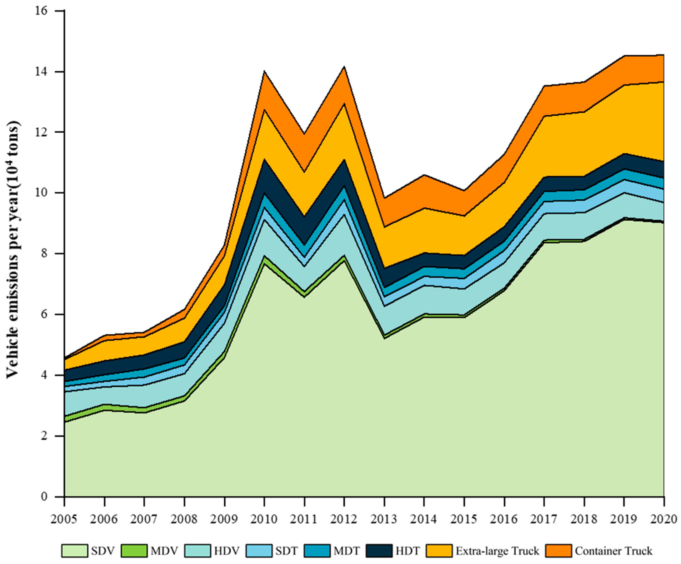
Based upon the COPERT model, the multi-year expressway vehicle emission inventories of four pollutants (i.e., CO, VOC, NOx, and PM) in the JZH region from 2005 to 2020 are obtained. Figure 6 illustrates the total expressway vehicle emission trends by eight vehicle types. In general, fluctuations have been observed in the overall trend of total emissions for four pollutants, with the early peaks occurring in 2010 and 2013, and afterwards rising to reach the latest peak in 2020. This phenomenon may be attributed to the update frequency of vehicle emission standards. For example, emission standards have been upgraded to China III since 2008 and to China IV since 2011, and as a result, the total emissions peak and have a downward trend in the following years, though VP is continuously increasing. Moreover, among these vehicle types, SDV is the dominant emission contributor, with 43.1 million tons emissions accounting for around 34.8% in the JZH region. For freight vehicle types, extra-large truck and container trainers have the highest percentage, contributing 21.3% and 11.6%, respectively.
Additionally, we compare the findings of our study to other regions in China analyzed in previous studies, i.e., the Harbin–Changchun Megalopolis (HCM) region, and the Yunnan–Guizhou Plateau (YGP) region [30,33,47]. Specifically, the similarities of these regions are that they both experienced a rapid growth period of vehicle emissions. Compared with the JZH region, the HCM region, which serve as one of China’s major centers for vehicle production industry, undergoes apparently larger seasonal emission changes due to its latitude located in Northeast China. During the winter season, the vehicle catalytic converters require more time to warm up; meanwhile, the slippery road decreased the engine combustion efficiency, both leading to increased vehicle emissions. As for the YGP region locating in Southwest China, compared with the JZH region, it is distinguished by its underdeveloped economy and predominant mountainous plateau landscape, resulting the more widely temporal difference of vehicle emissions within the region.

4.1.2. Analysis of Different Pollutants

The specific expressway vehicle emission compositions of four pollutants from eight vehicle types between 2005 and 2020 are shown in Figure 7. Among these pollutants, CO emission exhibits a relatively stable contribution, ranging between 23.1% to 27.2%. The PM emission contributes the least, with its range varying between 2.9% and 4.3%. VOC and NOx emissions present an opposite trend with respect to their contribution shifting over the 15 years. In 2005, VOC and NOx account for 26.1% and 42.7%, respectively, whereas the proportions are 40.7% and 33.6%, respectively, in 2020. Additionally, NOx and PM emissions exhibit a pattern of slowing down and stabilizing, which are mainly produced by passenger vehicles. In contrast, CO and VOC emissions show a fluctuating rising trend, which are primarily produced by freight vehicles, with HDT making up the main source of two pollutants.
For CO, as Figure 7a presents, the emission first peaks at roughly 47.2 thousand tons per year in 2010, then peaks again in 2017 after fluctuating and descending, until it eventually stabilizes at about 48 thousand tons per year. Among the eight vehicle types, SDV contributes 59.9% of the total CO emissions, emitting a total of 375 thousand tons from 2005 to 2020. Despite the fact that SDV has lower EF and lower individual vehicle emission compared to freight vehicles, the significant VP and higher VP growth rate have made it consistently contribute the most to CO emissions in the investigated 15 years. However, in terms of the extra-large trucks and container trucks, due to their rapid increase in VP, coupled with the fuel type of diesel and higher emissions per vehicle, their contribution to CO emissions has elevated, particularly in recent years.
For VOC, as Figure 7b depicts, the total emission has been rising more steadily and swiftly, from 12 thousand tons per year in 2005 to 59.2 thousand tons per year in 2020, with an increase of 395.0%. Among these, the contribution rate of VOC emissions from SDV is as high as 93.7%. Likewise, this is closely related to the high proportion of SDV in VP among various vehicle types, and the increase in new vehicle registrations, as VOC is mainly produced by synthetic materials, adhesives, and coatings used in vehicle decorations as well as inside parts like dashboards and seats.
For NOx, the total emission has witnessed a significant increment by 167.8% over a span of 15 years, rising from 12.4 thousand tons per year in 2005 to 33.3 thousand tons per year in 2020. Figure 7c illustrates that the main contributors to NOx emission are freight vehicles, including HDT, MDT, extra-large trucks, and container trucks. The possible reason is that these freight vehicles typically operate on diesel fuel, which have higher individual fuel consumption rates as compared to passenger vehicles.
For PM, as the trend and makeup of PM2.5 and PM10 are comparable, PM2.5 is used as an example in this section, as Figure 7d shows. PM10 is around 1.25 times that of PM2.5. The PM2.5 emission climbs quickly from 0.8 thousand tons per year in 2005 to 1.6 thousand tons per year in 2010, reaching its first peak. And, from 2017 to 2020, it stabilizes around 1.7 thousand tons per year. The distribution of emissions from HDT and other freight vehicle types is mostly uniform, with extra-large trucks contributing a comparatively high proportion of 24.1%. Moreover, despite the low EF, the contribution of PM2.5 emission from SDV rises steadily with the growing VP, reaching 19.5% by 2020.

4.2. Emission Control Policy Scenario Analysis

In this section, we employ policy scenario analysis to simulate the potential future trends of expressway vehicle emissions in the JZH region, setting a range of various development scenarios. According to Equation (1), VKT is given for each road segment in the JZH-ETS dataset, while VP and EF are two variable ingredients that impact the trends of expressway vehicle emissions in the future. The temporal variation of VP for different vehicle types is captured by the integrated SARIMA-SVR method. Meanwhile, the distribution of different vehicle types regarding predicted VP and the corresponding values of EF with various emission standards undergo changes with relatively uncertainties by implementing different emission control policies.

4.2.1. Results of VP Forecasting

The integrated SARIMA-SVR method is utilized to forecast the monthly VP, following the steps listed in Section 3.3. This study selects the monthly VP data from January 2005 to December 2018 as the training dataset, and the monthly VP data from January 2019 to December 2020 as the test dataset to predict the temporal variation of VP for different vehicle types from January 2021 to December 2030.
First and foremost, the original time series is examined for stationarity and white noise. Since the original dataset shows a clear periodicity and fails to pass the ADF test (ADF test statistic = −1.0800, p -value 0.05), first-order trend differencing and seasonal differencing with periods 1 and 12 are applied. The differenced dataset exhibits irregular fluctuations with a mean of zero, effectively eliminating both the trend and the seasonality, and passes the ADF test (ADF test statistic = −3.8917, p -value = 0.0021 < 0.05). Additionally, the differenced dataset also passes the test for white noise ( p -value = 0.000002 0.05), indicating that the dataset is non-white noise and contains the necessary information for modeling.
To optimize the parameter determination process for the SARIMA model, auto-correlogram, and partial-correlogram are generated for the pre-processed sample. Based on the plots, a parameter set is defined, and then, the optimal parameters are identified by the Grid Search method that the best combination is S A R I M A ( 2,1 , 2 ) × ( 1,1 , 1 ) 12 with an AIC statistic of 3067.19.
Subsequently, the SVR module is executed. A range of orders from 2 to 40 is considered to determine the sliding window length for predicting the residual sequence. After conducting multiple experiments, a sliding window length of 28 is identified as the optimal choice. The radial basis function (RBF) is chosen as the kernel function for the SVR model, and the Grid Search method is conducted to determine the optimal parameters combination with C = 2.5354 and γ = 0.0335. Then, rolling training and prediction are performed to better simulate unexpected fluctuations that may occur in the time series. Lastly, the SARIMA predicted sequence and the SVR residual fitted sequence are integrated to predict the monthly VP in the future.
Results indicate that the estimation for the peak values of VP using the SARIMA model is not sufficiently precise, while the residual errors can be effectively reduced when the SVR module is incorporated. The monthly relative errors, overall mean absolute percentage error (MAPE), and symmetric mean absolute percentage error (SMAPE) are computed in order to assess the model performance, as shown in Table 1 and Table 2. It shows a clear effect that the integrated SARIMA-SVR method, which is corrected by the SVR rolling residual prediction, has an improved predictive capability and can reflect the trend and seasonality of the time series.

4.2.2. Scenario Settings

Based on the existing literature (e.g., [4,37]), this study considers three emission control policies, including the constraint policy of VP, the update frequency of emission standards influencing EF, and the scrapping policy of high-emission vehicles. Policy A aims to control the growth of VP through restrictions, along with the adjustments and upgrading of the medium- and long-haul transportation structures. It contains three specific measures, which are the natural VP growth measure (A1), the moderate VP constrained measure (A2), and the aggressive VP constrained measure (A3), corresponding to no VP restriction, and a 5% and 10% reduction in VP, respectively. Policy B considers the update frequency of emission standards. The interval for updating standards is set to low frequency (B1), medium frequency (B2), and high frequency (B3), corresponding to updating every 4, 3, and 2 years, respectively. Policy C features the scrapping policy for high-emission vehicles. It is split into natural elimination measure (C1), moderate elimination measure (C2), and an aggressive elimination measure (C3), corresponding to natural scrapping vehicles, and an additional elimination of 5% and 10% of high-emission vehicles with emission standards earlier than China VI, respectively. The combination of three policies constitutes a set of different scenarios. Specifically, by applying the orthogonal experimental design method, nine representative scenarios are established. The specific settings of these scenarios are outlined in Table 3.
The detailed characteristics of nine scenarios in Table 3 are illustrated as follows.
Scenario 1
As the baseline scenario, Scenario 1 assumes the natural growth of VP according to the historical and current variation tendency, and low-frequency update to the prevailing emission standards, and natural elimination of vehicles without extra scrapping.
Scenario 2
Among the nine scenarios, Scenario 2 exhibits a mild level of emission reduction. Without limiting VP development, it adopts a moderate frequency for updating emission standards, but has a strict strategy for eliminating the high-emission vehicles.
Scenario 3
This scenario presents a similar effectiveness of emission reduction as Scenario 2. It takes relatively minor measures for Policy A and C, enabling VP to naturally expand and modestly reduce the high-emission vehicles. However, it adopts a 2-year update interval for the emission standards.
Scenario 4
Compared to the baseline scenario, this scenario displays the least effective emission reduction, executing an aggressive measure to eliminate high-emission vehicles, while applying a moderate VP constraint policy. Additionally, the update frequency of emission standards is 4 years.
Scenario 5
The regulatory actions taken in this scenario are generally of a moderate level, with all three policies implementing the medium measures.
Scenario 6
In this scenario, which ranks second in terms of the emission reduction effect, the moderate VP constraint policy is adopted, combined with a natural vehicle elimination program, while taking the 2-year interval for updating emission standards.
Scenario 7
This scenario shows a reasonable emission reduction effectiveness during the early phase of policy implementation, but gradually loses it advantage in the middle and later period. It enforces stringent VP constraint policy and moderate elimination policy, but only updates emission standards every 4 years.
Scenario 8
In contrast to Scenario 7, this scenario displays a modest emission level throughout the early phase, but performs well in the middle and later periods. It employs a moderate update frequency for emission standards, strictly implements VP restriction policy, and does not apply extra vehicle elimination measures.
Scenario 9
In this best achieved emission reduction scenario, the toughest measures for all three policies are enacted, including the aggressive VP constraint policy, the high frequency of updating emission standards, and the aggressive elimination policy for high-emission vehicles.

4.2.3. Analysis Results

The expressway vehicle emissions of pollutants in the JZH region from January 2021 to December 2030 are calculated by the COPERT model with the parameter adjustment of nine policy scenarios. Among them, Scenario 1 is the baseline scenario, with no restriction on VP growth, current emission standard updating frequency (low frequency), and the natural elimination of the vehicles. Figure 8 depicts the potential expressway vehicle emission trends of four pollutants in the JZH region between 2021 and 2030 under nine scenarios.
For CO, Scenario 9 presents the largest overall emission reduction effectiveness of 21.9% from January 2021 to December 2030 compared to baseline Scenario 1. Moreover, the peak emission occurs two years earlier in Scenario 9 than the baseline scenario, with a reduction of 20.6%. The differences in the emission reductions resulting from variations in scenario modes are more pronounced, as exhibited in Figure 8a. Overall, there is a declining trend, albeit with monthly fluctuations associated with the fluctuated monthly VP on the expressway. This is related to the fact that SDV contributes the most in CO emission because of its significant VP, leading better emission reduction effects under stringent VP control policies.
For VOC, as Figure 8b demonstrates, emission in the baseline scenario steadily varies downward from 2021 and inversely rises in 2030. In contrast, Scenario 9 likewise exhibits the most significant decrease in the amount of VOC emissions, with a reduction of 27.1% compared to the baseline scenario by December 2030. The reduction is attributed to the reasonable combination of shortening the frequency of updating emission standards, and scrapping high-emission vehicles.
For NOx, as Figure 8c shows, the emissions rise further, peaks in 2023, and then goes downward in the baseline scenario mode. In the baseline Scenario 1, NOx emission reaches a peak of 3.5 thousand tons per month in February 2023, and eventually decreases to 2.2 thousand tons per month by December 2030. Nevertheless, under the most stringent policy Scenario 9, the peak emission occurs earlier in February 2022 at 2.5 thousand tons per month, and gradually decreases to 1.6 thousand tons per month by December 2030. The peak and valley values in Scenario 9 present reductions of 28.4% and 27.3%, respectively, compared to the baseline Scenario 1. It can be attributed to the main contributing vehicle types of NOx emissions, namely HDT, MDT, extra-large trucks, and container trucks. Compared to passenger vehicles such as SDV, these freight vehicles have relatively shorter lifespans in general. Consequently, outdated and high-emission freight vehicles experience a sharp decline in VP under external policy regulations, leading to the significant emission reduction effectiveness and an early peak.
For PM, as Figure 8d indicates, in a similar vein, Scenario 9 delivers the highest decrease, with a reduction in the PM2.5 emission of 25.8% by December 2030 as compared against the baseline scenario. Moreover, among the four pollutants, PM exhibits the minimal variation in emission levels across different scenario modes. The possible reason may be its comparatively lower overall emission amount and the more evenly distributed contributions from different vehicle types.

5. Conclusions

Expressway systems play a pivotal role in intercounty passenger travel and freight mobility. This study takes the expressway vehicle emissions of the Jiang–Zhe–Hu (JZH) Region of China as the research objective. The COPERT model is used to establish the multi-year vehicle emission inventories of different pollutants in the JZH expressway system, covering the past and future trends from 2005 to 2030. The integrated SARIMA-SVR method is employed to capture the mechanism behind the temporal variation of VP. Further, with different levels of various policy scenarios considered, a set of scenarios are generated. The combination of monthly VP forecasting and scenario analysis can more accurately grasp the potential diversity of expressway vehicle emission development trends in the JZH region. The main conclusions of this study are as follows:
  • The expressway vehicle emission inventories of the JZH region indicate that fluctuations have been observed in the overall trend of total emissions, with the early peaks occurring in 2010 and 2013, and afterwards rising to reach the latest peak in 2020. Regarding regional emission differences, emission inventories exhibit a shift in the primary source of expressway vehicle emissions from Jiangsu to Zhejiang during the 15 years investigated. Among the four pollutants, CO and VOC present a general upward trend, while NOx and PM display a slowing upward with fluctuations. Notably, CO and VOC emissions primarily originate from SDV, whereas NOx and PM emissions mainly source from freight vehicles, with extra-large trucks accounting for the highest proportion.
  • The integrated SARIMA-SVR method is capable of capturing both trend and seasonality in the monthly VP variation of different vehicle types, in which the SARIMA model extracts the linear information and the SVR module extracts the nonlinear information through rolling residual prediction. Later, the possible future evolution trends of expressway vehicle emissions are predicted through scenario analysis. Among the nine scenarios, Scenario 9 has the most significant emission reduction effectiveness, with a reduction in the total emission of four pollutants attaining 23.8% by December 2030 as compared against the baseline scenario.
Based upon the analysis results, this study suggests the following expressway vehicle emission reduction policies in the JZH region:
  • The multi-year expressway vehicle emission inventories presented in this study indicate that restrictions on the increase in VP is an effective policy measure to reduce the expressway vehicle emissions in the JZH region. Meanwhile, upgrading the medium- and long-haul transportation structure is necessitated to meet the continuous growth of intercity trips. Specifically, due to the lower unit mileage emissions by railways and waterways, constructing and optimizing the corresponding transportation infrastructures are beneficial to shift a portion of freight transport from expressways to railways and waterways, and encourage more intercity travelers to switch from expressway to high-speed railways. In such cases, the constraint policy of VP can promote the multimodal transport development and contribute to the expressway vehicle emission reduction in a sustainable way.
  • Furthermore, it is also necessary to take appropriate intervals for updating the emission standards and gradually phase out the outdated vehicles to alter the proportion of vehicles with various emission standards, and encourage the advancements in vehicle emission control technologies in the JZH region. The improvement in tail gas treatment, fuel quality and engine design are all key indicators for effectively decreasing the emissions, and considerably enhance the air quality. For vehicles which emissions are not up to the standard, strict verification and inspection should be performed. Additionally, for vehicles that have high mileage with outdated emission standards, measures comprise incentive and subsidy might be utilized to encourage the public to voluntarily register the vehicles for elimination and recycling. Generally, more effective sustainability and expressway vehicle emission reduction effectiveness can be enhanced by the emission standard updating policy, along with the high-emission vehicle elimination policy.
Admittedly, this study comes with some limitations, and the following improvements are suggested: (i) Integration of electric and hybrid vehicles in the model to provide a more comprehensive view and possibly suggest more sustainable solutions for the future. (ii) In-depth analysis with real-world measurements could further improve the computational accuracy of vehicle emissions. (iii) When the ETS datasets of more regions in China are available, the similarities and differences of expressway vehicle emissions between these regions could be systematically compared. The authors recommend that future studies could focus on these issues.

Author Contributions

Conceptualization, J.C. (Jingxu Chen) and D.C.; methodology, J.C. (Jingxu Chen) and J.C. (Junyi Chen); software, J.C. (Junyi Chen) and X.S.; validation, J.C. (Junyi Chen), D.C. and X.S.; formal analysis, J.C. (Jingxu Chen) and J.C. (Junyi Chen); investigation, X.S. and D.C.; data curation, D.C.; writing—original draft preparation, J.C. (Jingxu Chen), J.C. (Junyi Chen), D.C. and X.S.; writing—review and editing, J.C. (Jingxu Chen), J.C. (Junyi Chen) and X.S.; visualization, J.C. (Junyi Chen), X.S.; project administration, D.C. All authors have read and agreed to the published version of the manuscript.

Funding

This work is supported by the Transportation Science and Technology Project of Henan Province, China (2023-2-2).

Data Availability Statement

Data will be made available upon request from the corresponding author.

Acknowledgments

The authors would like to thank the students from the School of Transportation, Southeast University, for their help in data collection and suggestions on the manuscript.

Conflicts of Interest

The authors declare no conflicts of interest.

References

  1. The Total Number of Vehicles in China Reaches 417 Million, and the Number of Drivers Exceeds 500 Million. Available online: https://www.gov.cn/xinwen/2023-01/11/content_5736278.htm (accessed on 12 January 2023). (In Chinese)
  2. Guo, X.; Zhang, X.; Dong, J.; Yang, X. Optimal Allocation of Urban New Energy Vehicles and Traditional Energy Vehicles Considering Pollution and Cost. Environment, Dev. Sustain. 2024, 26, 6007–6026. [Google Scholar] [CrossRef]
  3. Wu, Y.; Zhang, S.; Hao, J.; Liu, H.; Wu, X.; Hu, J.; Walsh, M.P.; Wallington, T.J.; Zhang, K.M.; Stevanovic, S. On-Road Vehicle Emissions and Their Control in China: A Review and Outlook. Sci. Total Environ. 2017, 574, 332–349. [Google Scholar] [CrossRef] [PubMed]
  4. Liu, G.; Sun, S.; Zou, C.; Wang, B.; Wu, L.; Mao, H. Air Pollutant Emissions from On-Road Vehicles and Their Control in Inner Mongolia, China. Energy 2022, 238, 121724. [Google Scholar] [CrossRef]
  5. Zheng, B.; Tong, D.; Li, M.; Liu, F.; Hong, C.; Geng, G.; Li, H.; Li, X.; Peng, L.; Qi, J.; et al. Trends in China’s Anthropogenic Emissions since 2010 as the Consequence of Clean Air Actions. Atmos. Chem. Phys. 2018, 18, 14095–14111. [Google Scholar] [CrossRef]
  6. Song, W.; Zhang, X.; An, K.; Yang, T.; Li, H.; Wang, C. Quantifying the Spillover Elasticities of Urban Built Environment Configurations on the Adjacent Traffic CO2 Emissions in Mainland China. Appl. Energy 2021, 283, 116271. [Google Scholar] [CrossRef]
  7. China’s Cumulative Expressway Mileage from 1988 to 2021. Available online: https://m.shujujidi.com/hangye/163.html (accessed on 30 January 2023). (In Chinese).
  8. Li, H.; Liu, Y.; Peng, K. Characterizing the Relationship between Road Infrastructure and Local Economy Using Structural Equation Modeling. Transp. Policy 2018, 61, 17–25. [Google Scholar] [CrossRef]
  9. Comprehensive Review of Expressway Mileage in Various Provinces. Available online: https://www.chinahighway.com/article/65395403.html (accessed on 30 January 2023). (In Chinese).
  10. Tian, Y. Mutualistic Pattern of Intra-Urban Agglomeration and Impact Analysis: A Case Study of 11 Urban Agglomerations of Mainland China. ISPRS Int. J. Geo-Inf. 2020, 9, 565. [Google Scholar] [CrossRef]
  11. Li, M.; Liu, H.; Geng, G.; Hong, C.; Liu, F.; Song, Y.; Tong, D.; Zheng, B.; Cui, H.; Man, H.; et al. Anthropogenic Emission Inventories in China: A Review. Natl. Sci. Rev. 2017, 4, 834–866. [Google Scholar] [CrossRef]
  12. Zhang, L.; Long, R.; Chen, H.; Geng, J. A Review of China’s Road Traffic Carbon Emissions. J. Clean. Prod. 2019, 207, 569–581. [Google Scholar] [CrossRef]
  13. Sun, S.; Sun, L.; Liu, G.; Zou, C.; Wang, Y.; Wu, L.; Mao, H. Developing a Vehicle Emission Inventory with High Temporal-Spatial Resolution in Tianjin, China. Sci. Total Environ. 2021, 776, 145873. [Google Scholar] [CrossRef]
  14. Song, X.; Hao, Y.; Zhang, C.; Peng, J.; Zhu, X. Vehicular Emission Trends in the Pan-Yangtze River Delta in China between 1999 and 2013. J. Clean. Prod. 2016, 137, 1045–1054. [Google Scholar] [CrossRef]
  15. Jiang, P.; Zhong, X.; Li, L. On-Road Vehicle Emission Inventory and Its Spatio-Temporal Variations in North China Plain. Environ. Pollut. 2020, 267, 115639. [Google Scholar] [CrossRef]
  16. Zhu, C.; Qu, X.; Qiu, M.; Zhu, C.; Wang, C.; Wang, B.; Sun, L.; Yang, N.; Yan, G.; Xu, C.; et al. High Spatiotemporal Resolution Vehicular Emission Inventory in Beijing-Tianjin-Hebei and Its Surrounding Areas (BTHSA) during 2000–2020, China. Sci. Total Environ. 2023, 873, 162389. [Google Scholar] [CrossRef]
  17. Parrish, D.D. Critical Evaluation of US On-Road Vehicle Emission Inventories. Atmos. Environ. 2006, 40, 2288–2300. [Google Scholar] [CrossRef]
  18. Progiou, A.G.; Ziomas, I.C. Road Traffic Emissions Impact on Air Quality of the Greater Athens Area Based on a 20 Year Emissions Inventory. Sci. Total Environ. 2011, 410, 1–7. [Google Scholar] [CrossRef] [PubMed]
  19. McDonald, B.C.; Gentner, D.R.; Goldstein, A.H.; Harley, R.A. Long-Term Trends in Motor Vehicle Emissions in US Urban Areas. Environ. Sci. Technol. 2013, 47, 10022–10031. [Google Scholar] [CrossRef] [PubMed]
  20. Pallavidino, L.; Prandi, R.; Bertello, A.; Bracco, E.; Pavone, F. Compilation of a Road Transport Emission Inventory for the Province of Turin: Advantages and Key Factors of a Bottom–up Approach. Atmos. Pollut. Res. 2014, 5, 648–655. [Google Scholar] [CrossRef]
  21. Dey, S.; Caulfield, B.; Ghosh, B. Modelling Uncertainty of Vehicular Emissions Inventory: A Case Study of Ireland. J. Clean. Prod. 2019, 213, 1115–1126. [Google Scholar] [CrossRef]
  22. Cai, H.; Xie, S. Estimation of Vehicular Emission Inventories in China from 1980 to 2005. Atmos. Environ. 2007, 41, 8963–8979. [Google Scholar] [CrossRef]
  23. Lang, J.; Cheng, S.; Zhou, Y.; Zhang, Y.; Wang, G. Air Pollutant Emissions from On-Road Vehicles in China, 1999–2011. Sci. Total Environ. 2014, 496, 1–10. [Google Scholar] [CrossRef]
  24. Yang, X.; Liu, H.; Man, H.; He, K. Characterization of Road Freight Transportation and Its Impact on the National Emission Inventory in China. Atmos. Chem. Phys. 2015, 15, 2105–2118. [Google Scholar] [CrossRef]
  25. Wu, X.; Wu, Y.; Zhang, S.; Liu, H.; Fu, L.; Hao, J. Assessment of Vehicle Emission Programs in China during 1998–2013: Achievement, Challenges and Implications. Environ. Pollut. 2016, 214, 556–567. [Google Scholar] [CrossRef]
  26. Jia, T.; Li, Q.; Shi, W. Estimation and Analysis of Emissions from On-Road Vehicles in Mainland China for the Period 2011–2015. Atmos. Environ. 2018, 191, 500–512. [Google Scholar] [CrossRef]
  27. Lang, J.; Cheng, S.; Wei, W.; Zhou, Y.; Wei, X.; Chen, D. A Study on the Trends of Vehicular Emissions in the Beijing–Tianjin–Hebei (BTH) Region, China. Atmos. Environ. 2012, 62, 605–614. [Google Scholar] [CrossRef]
  28. Guo, X.; Fu, L.; Ji, M.; Lang, J.; Chen, D.; Cheng, S. Scenario Analysis to Vehicular Emission Reduction in Beijing-Tianjin-Hebei (BTH) Region, China. Environ. Pollut. 2016, 216, 470–479. [Google Scholar] [CrossRef] [PubMed]
  29. Yang, W.; Yu, C.; Yuan, W.; Wu, X.; Zhang, W.; Wang, X. High-Resolution Vehicle Emission Inventory and Emission Control Policy Scenario Analysis, a Case in the Beijing-Tianjin-Hebei (BTH) Region, China. J. Clean. Prod. 2018, 203, 530–539. [Google Scholar] [CrossRef]
  30. Gao, C.; Gao, C.; Song, K.; Xing, Y.; Chen, W. Vehicle Emissions Inventory in High Spatial–Temporal Resolution and Emission Reduction Strategy in Harbin-Changchun Megalopolis. Process Saf. Environ. Prot. 2020, 138, 236–245. [Google Scholar] [CrossRef]
  31. Liu, Y.-H.; Liao, W.-Y.; Li, L.; Huang, Y.-T.; Xu, W.-J. Vehicle Emission Trends in China’s Guangdong Province from 1994 to 2014. Sci. Total Environ. 2017, 586, 512–521. [Google Scholar] [CrossRef] [PubMed]
  32. Sun, S.; Jiang, W.; Gao, W. Vehicle Emission Trends and Spatial Distribution in Shandong Province, China, from 2000 to 2014. Atmos. Environ. 2016, 147, 190–199. [Google Scholar] [CrossRef]
  33. Lv, W.; Hu, Y.; Li, E.; Liu, H.; Pan, H.; Ji, S.; Hayat, T.; Alsaedi, A.; Ahmad, B. Evaluation of Vehicle Emission in Yunnan Province from 2003 to 2015. J. Clean. Prod. 2019, 207, 814–825. [Google Scholar] [CrossRef]
  34. Zhang, S.; Wu, Y.; Wu, X.; Li, M.; Ge, Y.; Liang, B.; Xu, Y.; Zhou, Y.; Liu, H.; Fu, L.; et al. Historic and Future Trends of Vehicle Emissions in Beijing, 1998–2020: A Policy Assessment for the Most Stringent Vehicle Emission Control Program in China. Atmos. Environ. 2014, 89, 216–229. [Google Scholar] [CrossRef]
  35. Wu, T.; Cui, Y.; Lian, A.; Tian, Y.; Li, R.; Liu, X.; Yan, J.; Xue, Y.; Liu, H.; Wu, B. Vehicle Emissions of Primary Air Pollutants from 2009 to 2019 and Projection for the 14th Five-Year Plan Period in Beijing, China. J. Environ. Sci. 2023, 124, 513–521. [Google Scholar] [CrossRef]
  36. Sun, S.; Zhao, G.; Wang, T.; Jin, J.; Wang, P.; Lin, Y.; Li, H.; Ying, Q.; Mao, H. Past and Future Trends of Vehicle Emissions in Tianjin, China, from 2000 to 2030. Atmos. Environ. 2019, 209, 182–191. [Google Scholar] [CrossRef]
  37. Sun, S.; Jin, J.; Xia, M.; Liu, Y.; Gao, M.; Zou, C.; Wang, T.; Lin, Y.; Wu, L.; Mao, H.; et al. Vehicle Emissions in a Middle-Sized City of China: Current Status and Future Trends. Environ. Int. 2020, 137, 105514. [Google Scholar] [CrossRef] [PubMed]
  38. Hao, Y.; Song, X. Research on Trends and Spatial Distribution of Vehicular Emissions and Its Control Measure Assessment in the Yangtze River Delta, China, for 1999–2015. Environ. Sci. Pollut. Res. 2018, 25, 36503–36517. [Google Scholar] [CrossRef]
  39. Xu, S.; Chan, H.K.; Zhang, T. Forecasting the Demand of the Aviation Industry Using Hybrid Time Series SARIMA-SVR Approach. Transp. Res. Part E Logist. Transp. Rev. 2019, 122, 169–180. [Google Scholar] [CrossRef]
  40. China Statistical Yearbook. 2021. Available online: https://www.stats.gov.cn/sj/ndsj/2021/indexch.htm (accessed on 26 March 2023). (In Chinese)
  41. Huo, H.; Wang, M. Modeling Future Vehicle Sales and Stock in China. Energy Policy 2012, 43, 17–29. [Google Scholar] [CrossRef]
  42. Hao, H.; Wang, H.; Ouyang, M.; Cheng, F. Vehicle Survival Patterns in China. Sci. China Technol. Sci. 2011, 54, 625–629. [Google Scholar] [CrossRef]
  43. He, K.; Huo, H.; Wang, Q.; Yao, Z. Technologic Method and Application of Vehicle Emission Calculation Model; China Science Publishing & Media: Beijing, China, 2014. (In Chinese) [Google Scholar]
  44. Yao, E.; Song, Y. Study on Eco-Route Planning Algorithm and Environmental Impact Assessment. J. Intell. Transp. Syst. 2013, 17, 42–53. [Google Scholar] [CrossRef]
  45. Zhao, T. Data-Driven Macro and Micro Traffic Simulation and Control Optimization for Expressways. Master’s Thesis, Guangdong University of Technology, Guangzhou, China, 2022. (In Chinese). [Google Scholar]
  46. Nobre, F.F.; Monteiro, A.B.S.; Telles, P.R.; Williamson, G.D. Dynamic Linear Model and SARIMA: A Comparison of Their Forecasting Performance in Epidemiology. Stat. Med. 2001, 20, 3051–3069. [Google Scholar] [CrossRef]
  47. Li, B.; Shi, X.F.; Liu, Y.P.; Lu, L.; Wang, G.L.; Thapa, S.; Qi, H. Long-term characteristics of criteria air pollutants in megacities of Harbin-Changchun megalopolis, Northeast China: Spatiotemporal variations, source analysis, and meteorological effects. Environ. Pollut. 2020, 267, 115441. [Google Scholar] [CrossRef] [PubMed]
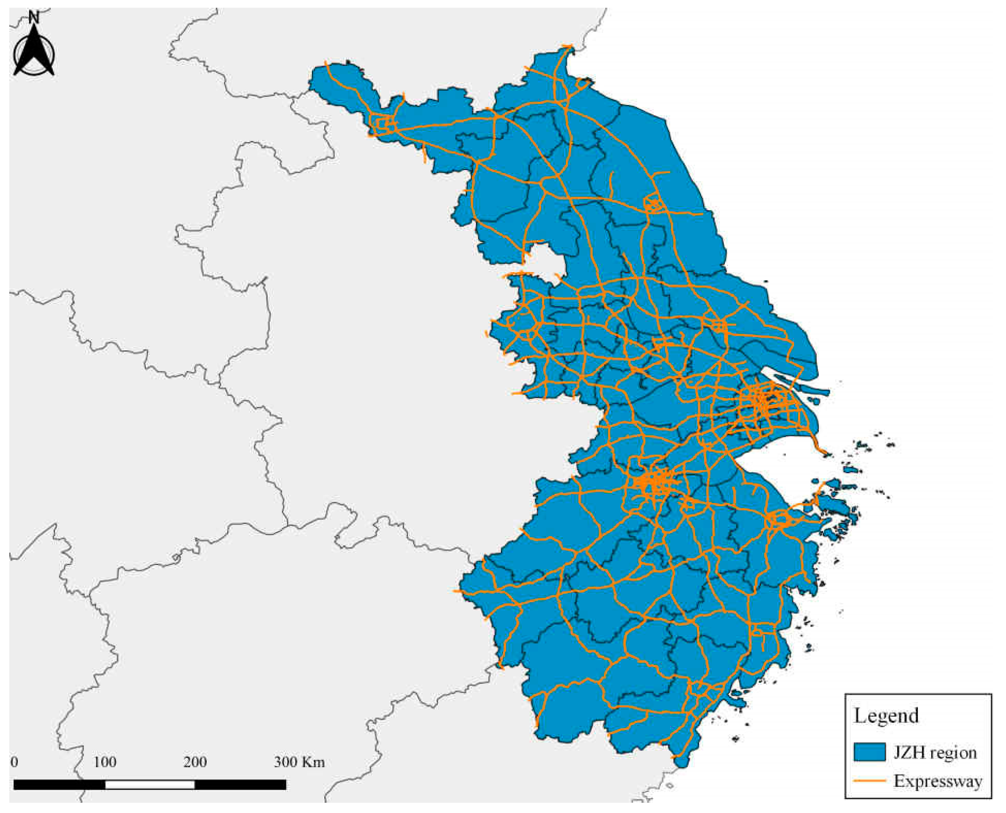
Figure 1. The expressway network of the JZH region.
Systems 12 00273 g001
Figure 2. Compositions of various vehicle emission standards from 2005 to 2020: (a) passenger vehicles; and (b) freight vehicles.
Systems 12 00273 g002
Figure 3. Flowchart of the integrated SARIMA-SVR method.
Systems 12 00273 g003
Figure 4. Research framework.
Systems 12 00273 g004
Figure 5. Expressway VP variation in the JZH region from 2005 to 2020.
Systems 12 00273 g005
Figure 6. Total emission trends by vehicle types in the JZH region from 2005 to 2020.
Systems 12 00273 g006
Figure 7. Emission compositions of eight vehicle types in the JZH region between 2005 and 2020: (a) CO; (b) VOC; (c) NOx; and (d) PM2.5.
Systems 12 00273 g007
Figure 8. Expressway vehicle emission trends of the JZH region between 2021 and 2030 under nine scenarios: (a) CO; (b) VOC; (c) NOx; and (d) PM2.5.
Systems 12 00273 g008
Table 1. Monthly relative errors of SARIMA and SARIMA-SVR models.
MonthRelative Errors of SARIMA (%)Relative Errors of SARIMA-SVR (%)
January 2019−18.78%−16.95%
February 20196.24%0.56%
March 20194.43%0.56%
April. 2019−6.57%−0.57%
May 20197.40%0.62%
June 2019−2.39%−0.54%
July 2019−10.57%−0.49%
August 2019−3.61%0.52%
September 2019−7.80%−0.51%
October 2019−7.11%−0.63%
November 2019−4.01%−0.55%
December 2019−5.85%−0.54%
January 2020−5.52%0.04%
February 202011.12%0.58%
March 202010.90%0.58%
April 2020−0.28%0.58%
May 2020−4.76%−0.53%
June 2020−1.41%−0.53%
July 20203.58%0.55%
August 20207.10%0.56%
September 20205.07%0.56%
October 2020−5.73%−0.62%
November 2020−1.72%−0.35%
December 20202.95%−0.58%
Table 2. Overall accuracy of SARIMA and SARIMA-SVR methods.
ModelMAPESMAPE
SARIMA7.06%6.54%
SARIMA-SVR1.27%1.21%
Table 3. Scenario settings.
ScenarioPolicy APolicy BPolicy C
Scenario 1Natural (A1)Low (B1)Natural (C1)
Scenario 2Natural (A1)Medium (B2)Aggressive (C3)
Scenario 3Natural (A1)High (B3)Moderate (C2)
Scenario 4Moderate (A2)Low (B1)Aggressive (C3)
Scenario 5Moderate (A2)Medium (B2)Moderate (C2)
Scenario 6Moderate (A2)High (B3)Natural (C1)
Scenario 7Aggressive (A3)Low (B1)Moderate (C2)
Scenario 8Aggressive (A3)Medium (B2)Natural (C1)
Scenario 9Aggressive (A3)High (B3)Aggressive (C3)
Disclaimer/Publisher’s Note: The statements, opinions and data contained in all publications are solely those of the individual author(s) and contributor(s) and not of MDPI and/or the editor(s). MDPI and/or the editor(s) disclaim responsibility for any injury to people or property resulting from any ideas, methods, instructions or products referred to in the content.