1. Introduction
As a basic material for human survival, grain is a cornerstone in the development of human civilization. It is very important for social stability and economic development.
In comparison to general commodity prices, agricultural commodity prices are subject to a more intricate array of factors such as income levels, international oil prices, grain supply and demand conditions, and market speculation [
1] and display irregular fluctuations, characterized by non-stationarity and non-linearity [
2]. Violent price fluctuations will have a bad effect on farmer’s production decision making and people’s consumption, and may even cause uneven development of the national economy [
3].
Thus, forecasting the grain futures price is of great importance for farmers, food supply chain participants, governments, and regulators [
4]. Through effective forecasting, we can better cope with market fluctuations, make reasonable decisions, and promote the sustainable development of the food industry. However, due to the complex influence of multiple factors, grain futures price prediction is still a challenging field, and continuous research and innovation are needed to improve the accuracy and reliability of the prediction.
There are mainly three prediction methods in the field of time series: traditional econometric methods, artificial intelligence methods based on machine learning or deep learning, and combined prediction methods. The traditional econometric model has high requirements for data stationarity, and data with great volatility may lead to unstable prediction results and poor prediction performance on long time series data [
5,
6].
Compared with traditional econometric models, artificial intelligence models can achieve better prediction results in the face of large-scale data with many relevant features [
7]. Typical representative models include artificial neural networks (ANNs), long short-term memory neural networks (LSTM), etc. The work [
8] compares the errors of the LSTM, TDNN, and ARIMA models in forecasting the international monthly prices of corn and palm oil and finds that the errors of the LSTM model are smaller than ARIMA and the TDNN. Jiang Zhihang applied BiLSTM to predict cotton price and achieved a lower error than LSTM [
9].
Researchers have applied the temporal convolutional network (TCN) model to predict pork prices and found the prediction effect of the TCN to be more obvious when dealing with large quantities of data [
10]. The work [
11] used ConvLSTM to predict the stock market. Compared with the classical LSTM model, the prediction accuracy of ConvLSTM is higher.
Although these methods have achieved good results in their respective fields, they all have certain limitations in application. For example, the LSTM network will lose the sequence feature information in the face of long time series, and there will also be the problem of disordered structural information between data [
12]. BiLSTM can obtain global context information through the bidirectional structure, which can capture the overall sequence pattern, but it will ignore some local features [
13]. Similarly, ConvLSTM is not effective in dealing with time series with long-term dependencies, and its complex model structure will lead to poor interpretability [
14]. So, a single model has difficulty grasping the relevant dependencies in the time series [
15], can be misleading, and is subject to at least three sources of uncertainty: data uncertainty, parameter uncertainty, and model uncertainty [
16]. Therefore, it is difficult to find a single model that applies to all situations [
17].
To this end, researchers have tried to combine multiple models for prediction. Sun combined variational mode decomposition (VMD), ensemble empirical mode decomposition (EEDM), and LSTM and used VMD and EEDM to perform decomposition twice to reduce the data complexity, which was combined as the VMD-EEMD-LSTM model [
18]. In view of the complexity and long-term dependence of stock prices, Lu proposed a futures-price-prediction model combining a CNN and LSTM and introduced the attention mechanism to optimize the model. Compared with the RNN, MLP, CNN, LSTM, CNN-RNN, and other benchmark models, the accuracy was improved [
19].
Researchers have also tried to introduce attention mechanisms, which are always combined with deep learning models [
20,
21], such as multi-head attention [
22] and self-attention [
23]. The attention mechanism has the advantage of overcoming the issues of long-term dependencies and information loss in recurrent neural networks [
24]. It assigns a different importance to each element in the input sequence and focuses on the inputs with stronger correlations, thus better representing the input data. Sun used models such as the SWS-CNN to predict the rise and fall of financial assets and found that the SWS-CNN-Attention model, which had the attention mechanism added to it, on the basis of the SWS-CNN, performed better, with a higher accuracy, precision, recall rate, and F1-score than other simple deep learning models [
25]. The work [
26] combines a CNN, BiLSTM, and attention mechanism to solve the problem of information loss caused by a time series data input that is too long. The CNN-BiLSTM-Attention model had a significant improvement in the accuracy compared with the single LSTM, CNN-BiLSTM, CNN-LSTM, CNN, and other models.
In summary, combined models can effectively utilize information from the sample data, overcome the drawbacks of single models, and provide a more comprehensive and accurate prediction. They facilitate the integration of useful information from various methods, thereby improving prediction accuracy [
27]. However, the combined models bring about new problems. The structure of combined models is more complex. This complexity will raise the cost of prediction and raise additional challenges for the practical deployment and application of the prediction models. Moreover, the performance of the model can vary significantly with respect to different datasets or conditions due to the substantial impact of random factors.
In order to enhance the accuracy and efficiency of the prediction model and support reasonable decision making, this paper considers the rationality of data feature selection and model combination to further improve the prediction performance, especially in the face of long-term time series prediction tasks, and proposes a grain futures price prediction model based on BiLSTM, DSConvLSTM, and an attention mechanism. The main work is as follows:
- (1)
Feature selection optimization: Calculate the mutual information value between each feature (the influence factor of grain futures price) and the futures price, then sort each feature according to the mutual information value; finally, determine the optimal number of features to select through comparative experiments instead of the traditional artificial setting or a theoretical hypothesis.
- (2)
Lightweight improvement: A more lightweight depthwise separable convolution (DSConv) was introduced to replace the standard convolution (SConv) in ConvLSTM, which can reduce the complexity of the model without sacrificing its performance [
28].
- (3)
Model combination: This paper proposes a combined model, Bi-DSConvLSTM-Attention, for grain futures price prediction; the BiLSTM and DSConvLSTM neural network models are combined to make full use of the respective advantages of the two models, and the attention mechanism is introduced to enhance the model’s attention to relevant features by dynamically adjusting the weights of different time steps, so as to improve the accuracy and efficiency of grain futures price prediction.
- (4)
Comparative analysis of model performance: This paper first takes the wheat futures price as an example to determine the specific attention mechanism. Then, taking wheat futures price prediction as an example, through comparative experiments, the Bi-ConvLSTM-Attention, LSTM, BiLSTM, LSTM-Attention, TCN-Attention, CNN-BiLSTM-Attention, and BiLSTM-Attention models were selected. The performance of the proposed model was compared with those of the above selected models. The best performance was achieved in terms of the root mean squared error (RMSE), mean absolute error (MAE), mean absolute percentage error (MAPE), and coefficient of determination ().
- (5)
Generalization capability test: The soybean futures price was selected for the generalization experiment, and the experimental results showed that the Bi-DSConvLSTM-Attention model also achieved the best performance on various evaluation indicators.
2. Materials and Methods
The price prediction model is mainly divided into the preprocessing module, feature selection module, and prediction module. The original data are preprocessed in the preprocessing module; the mutual information method is used to evaluate the dependence of grain futures prices on each feature selected. Then, the data are divided into the training and test data sets. The Bi-DSConvLSTM-Attention model predicts the grain futures price based on the training data set. Finally, the test data set is used to test the performance of the model. The main process is shown in
Figure 1.
2.1. Mutual Information Feature Selection
There are many factors affecting the grain futures price, which will cause the “Curse of Dimensionality” problem in model training. In this paper, dimension reduction is carried out through feature selection. An ideal feature selection algorithm should remove irrelevant, weakly relevant, and redundant features, and retain non-redundant and strongly relevant features [
29]. For a variety of influencing factors in the data, the mutual information method is used for feature selection, and the optimal number of features is determined by comparative experiments on the model. The mutual information value is calculated as shown in Formula (
1).
where
Xi and
Y are continuous random variables,
n represents the total number of influencing factors of the grain futures price,
Xi represents the i-th factor among the influencing factors of the grain futures price,
Y represents the grain futures price,
p(
) represents the joint probability density function of random variables
Xi and
Y, and
p(
) and
p(
y) represent the marginal probability density function of
Xi and
Y, respectively.
The mutual information value is a measure of the correlation between the grain futures price Y and the factors affecting the grain futures price Xi; the larger the value, the greater the dependence between them.
2.2. Depthwise Separable Convolution
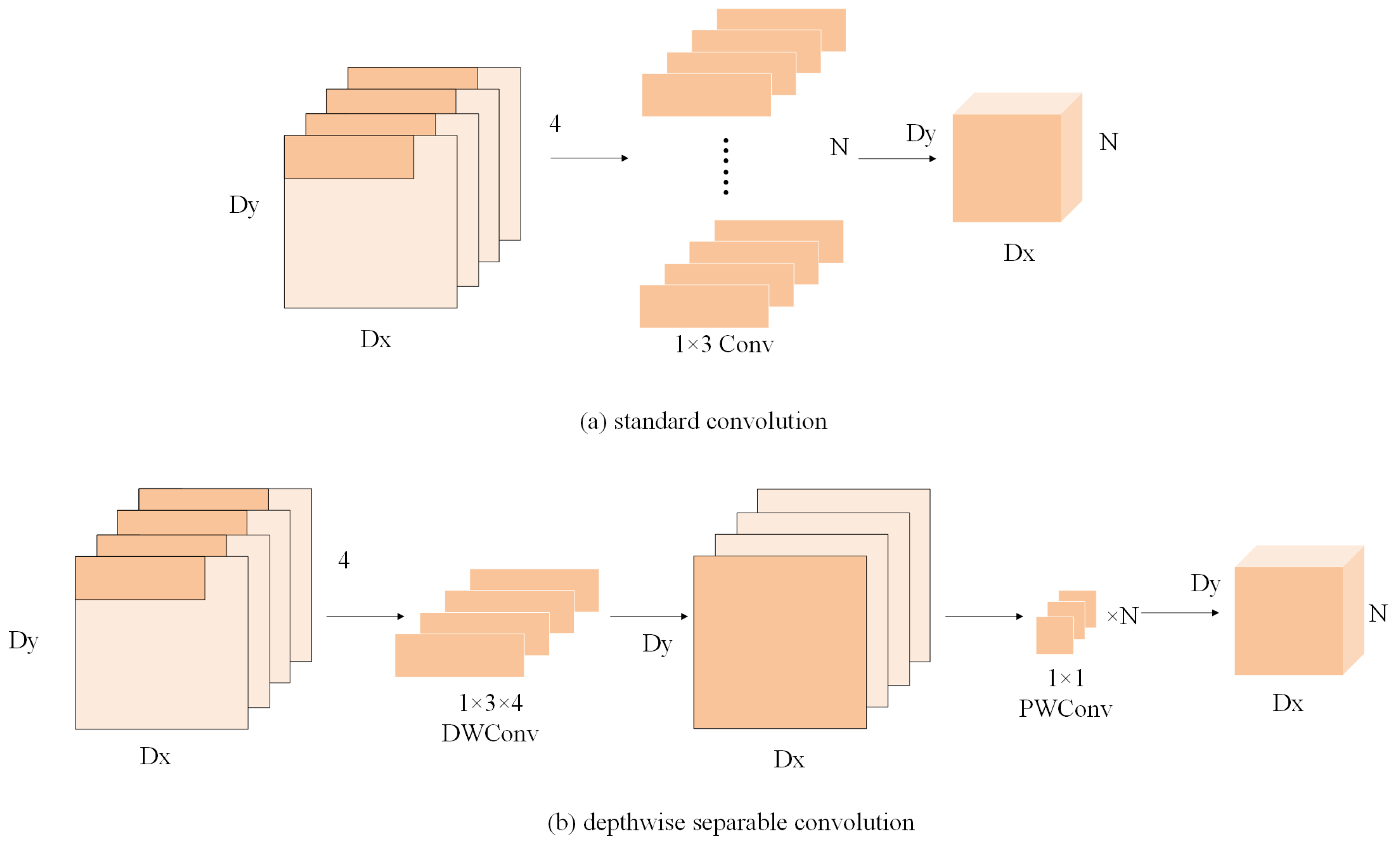
In contrast to the traditional convolution operation, depthwise separable convolution (DSConv) decomposes the traditional convolution operation into two parts: depthwise convolution (DWConv) and pointwise convolution (PWConv) [
30]. This approach can significantly reduce the number of parameters and computational cost of the model [
31], here taking the input of
as an example. This is shown in
Figure 2.
In the first step (DWConv), it applies a convolution kernel to each channel of the input feature map independently, without changing the number of channels; this operation has the same number of output channels as input channels. Then, in the second step (PWConv), it expands the number of channels to N channels by processing the output of DWConv with convolution kernels. Compared with the standard convolution process, the proposed method can significantly reduce the number of required parameters, where a combination of convolution kernels is applied to all channels of the feature map to directly produce a new feature map with N channels. The number of parameters required for the DSConv and standard convolution (SConv) processes can be calculated and compared using specific formulas.
SConvLSTM and DSConvLSTM have significant differences in the calculation of the number of parameters. Taking the convolution kernel of
as an example, The number of parameters is calculated as shown in Formulas (
2) and (
3), respectively.
In the formulas,
denotes the number of input channels and
denotes the number of output channels, and
is the bias term, which can be 0 or 1. We found that, since both
and
are greater than or equal to 1,
must be greater than
. See
Section 3.7 for detailed results.
2.3. Bi-DSConvLSTM-Attention
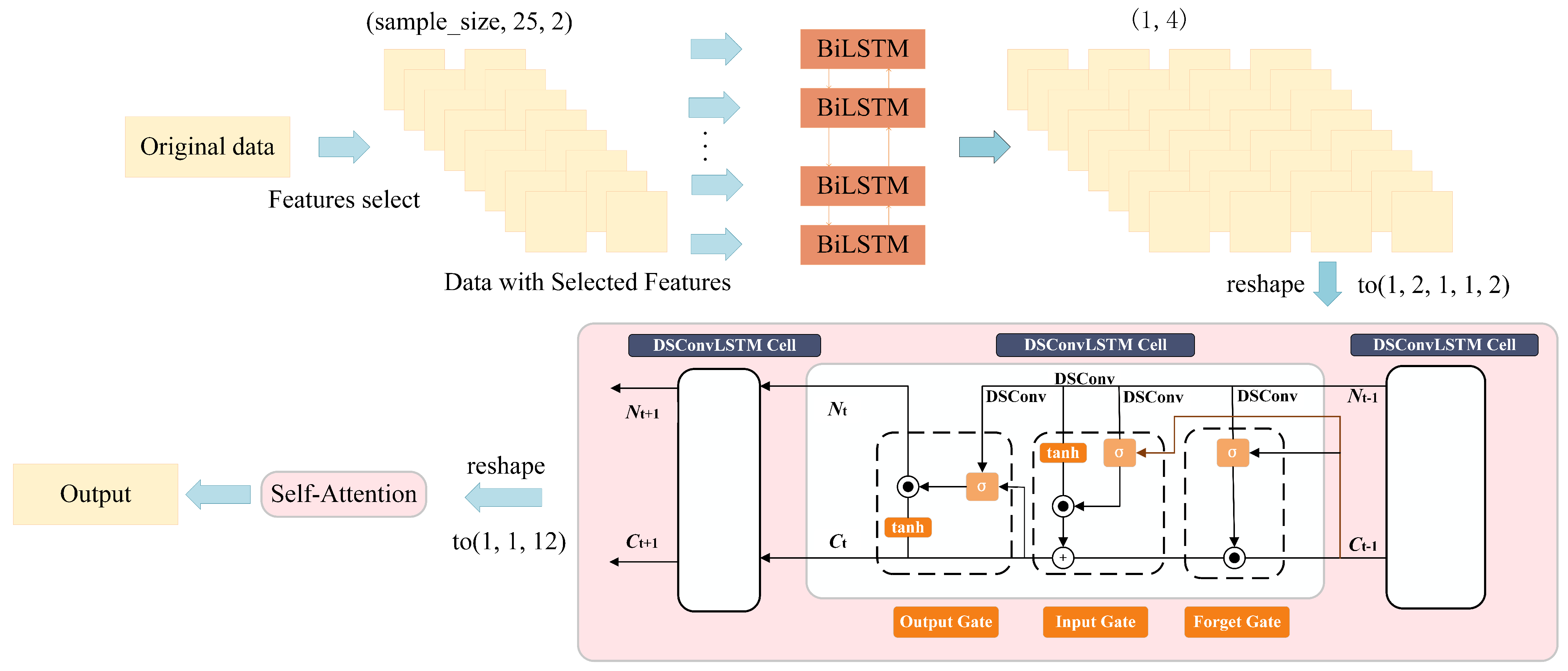
The bidirectional depthwise separable convolutional long short-term memory neural network model combined with the attention mechanism (Bi-DSConvLSTM-Attention) consists of BiLSTM, DSConvLSTM, and an attention layer. Its structure is shown in
Figure 3:
- (1)
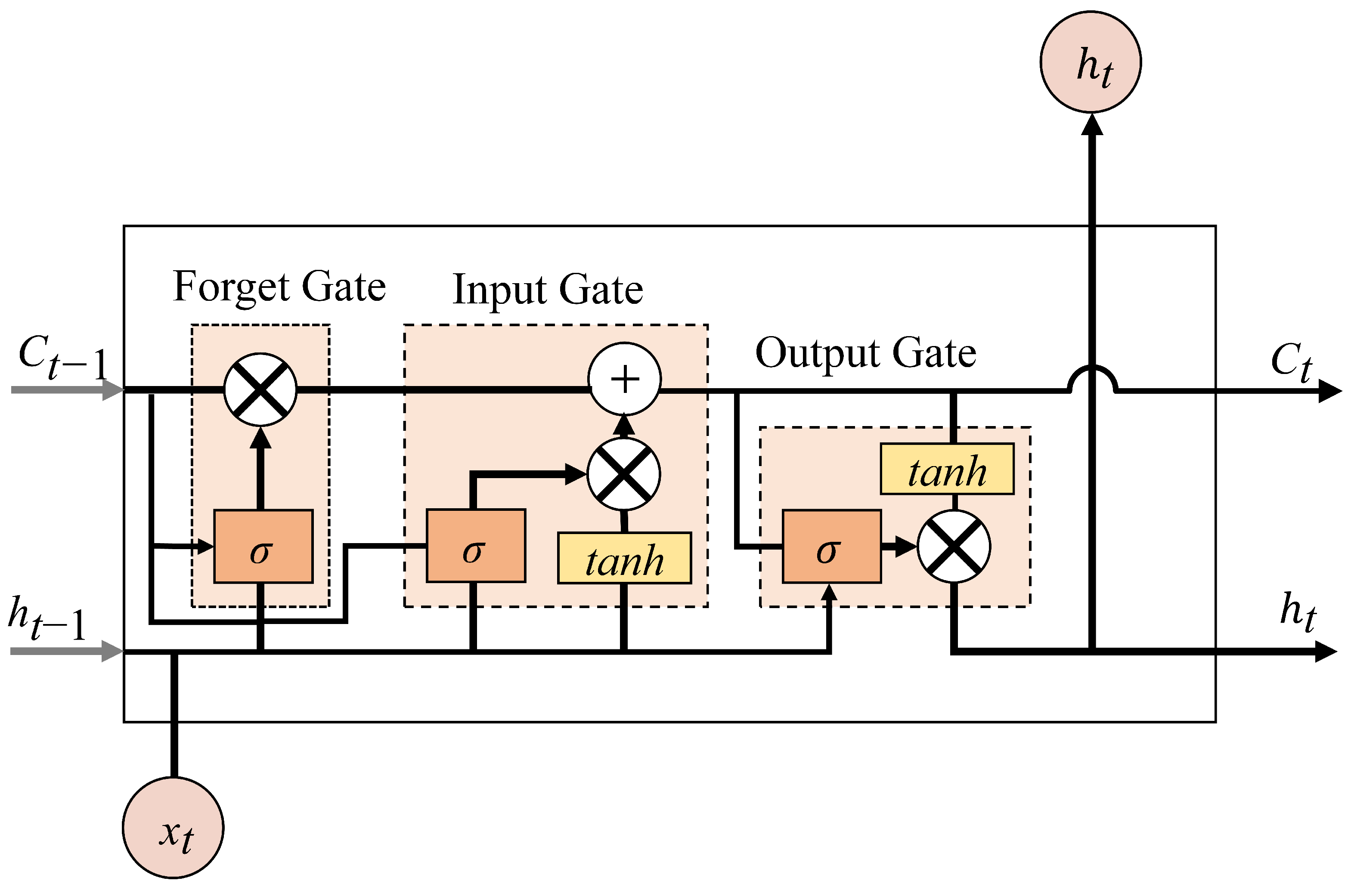
BiLSTM layer: By considering both forward and reverse information, it helps to fully understand the context in time series data and helps to improve the model’s ability to model time series patterns. BiLSTM consists of two LSTM layers: one LSTM layer processes the input sequence in order, and the other LSTM layer processes the input sequence in reverse order; finally, the outputs of the two LSTM layers are merged to obtain the complete context information at each time step. The LSTM unit structure is shown in
Figure 4.
The LSTM is calculated as follows:
where
represents the
sigmoid activation function,
represents the input data,
represents the previous time step’s output,
, and
represent the weight matrix multiplied by
, and
,
,
, and
represent the biases for
under the forget gate, cell state, input gate, and output gate, respectively.
,
,
, and
denote the weights for
under the forget gate, cell state, input gate, and output gate, respectively. By applying the hyperbolic tangent activation function tanh, we obtain the new candidate cell state
, and then, using Formula (
7), we compute the new cell state value.
After passing through the BiLSTM layer, the output h becomes , and this result is reshaped into a 5D tensor format required for the DSConvLSTM layer input.
- (2)
DSConvLSTM layer: DSConvLSTM introduces DSConv operations into the traditional LSTM recurrent structure, treating commodity futures prices as translations in the temporal direction. By leveraging the translation invariance property of convolution, DSConvLSTM can automatically learn spatial and temporal features in time series data, thereby improving the model’s performance and expressive power. We replace the fully connected layers in the LSTM with DSConv to capture local patterns in the sequence. The computation formula for DSConvLSTM is as follows:
The formula assumes that the current time step is t, the input is , the hidden state and the cell state at the previous time step are and , the output is , the cell state is , the input gate is , the forget gate is , the output gate is , and the candidate state is ; ⊗ represents the Hadamard product; * represents the convolution operation. , , and denote the convolution kernels for the input, hidden layer, and cell state, respectively, while , , , and denote the bias terms, respectively.
- (3)
Attention layer: The attention mechanism is widely used in natural language processing, image detection, speech recognition, and other fields [
32].
Attention consists of three main phases:
Phase 1: Calculate the similarity weight of each of the
data, as shown in Formula (
16).
Phase 2: Normalize the similarity weight by the
softmax function, as in Formula (
17).
Phase 3: The normalized similarity weights and their corresponding data are weighted and summed to obtain the output matrix R, as shown in Formula (
18).
where
denotes the connection weight matrix,
is the bias, and
and
, like
and
, denote the hidden state vector and its similarity weight at time
j, respectively.
The attention mechanism will enhance the model’s attention given to relevant features by dynamically adjusting the weights of different time steps, which is helpful to solve the problems of the performance degradation of neural networks caused by the increase of the input length and the low computational efficiency caused by the unreasonable input order.
2.4. Data Presentation
Considering the diversity of grains, and the wide application of wheat and soybean, the market is more transparent, so this paper takes wheat as an example to carry out the experiments. According to the literature [
33], this paper selects historical daily oil and natural gas prices and inflation indices from the Kaggle website [
34] and collects U.S. wheat, U.S. soybean, corn, and gold futures prices, as well as the exchange rate between USD and RMB, wheat output, and other data from websites such as
Investing.com (accessed on 23 July 2023). [
35]. Firstly, the data collected from different sources were integrated, and then, the data with missing values and outliers were deleted. Finally, 2118 wheat and soybean data were retained. The features possessed are shown in
Table 1, and there were 42 features. The training and test data sets were divided according to the ratio of 4:1, that is 1669 data in the training data set and 399 data in the test data set.
3. Analysis and Discussion
3.1. Evaluation Metrics
In order to accurately evaluate the model’s performance, this paper will use four indicators to evaluate the model: the root mean squared error (RMSE), mean absolute error (MAE), mean absolute percentage error (MAPE), and coefficient of determination (
). Their computed expressions are shown in Formulas (
19)–(
22), respectively.
In the formulas, n is the number of measurements, is the actual value of the i-th sample, and is the corresponding predicted value. SSE represents the sum of the squared differences between the actual observed values and the values predicted by the model. SST represents the sum of the squared differences between the actual observations and the mean of the observations.
3.2. Environment
The main software and third-party library versions used in the experiment were Python 3.6.13, Numpy 1.14.6, Pandas 1.0.5, Tensorflow 2.6.2, Scikit-learn 0.23.2, Keras 2.6.0, and Attention 4.1. After multiple training iterations, the parameters of the Bi-DSConvLSTM-Attention model in the experiment were set as shown in
Table 2.
3.3. Feature Selection Analysis
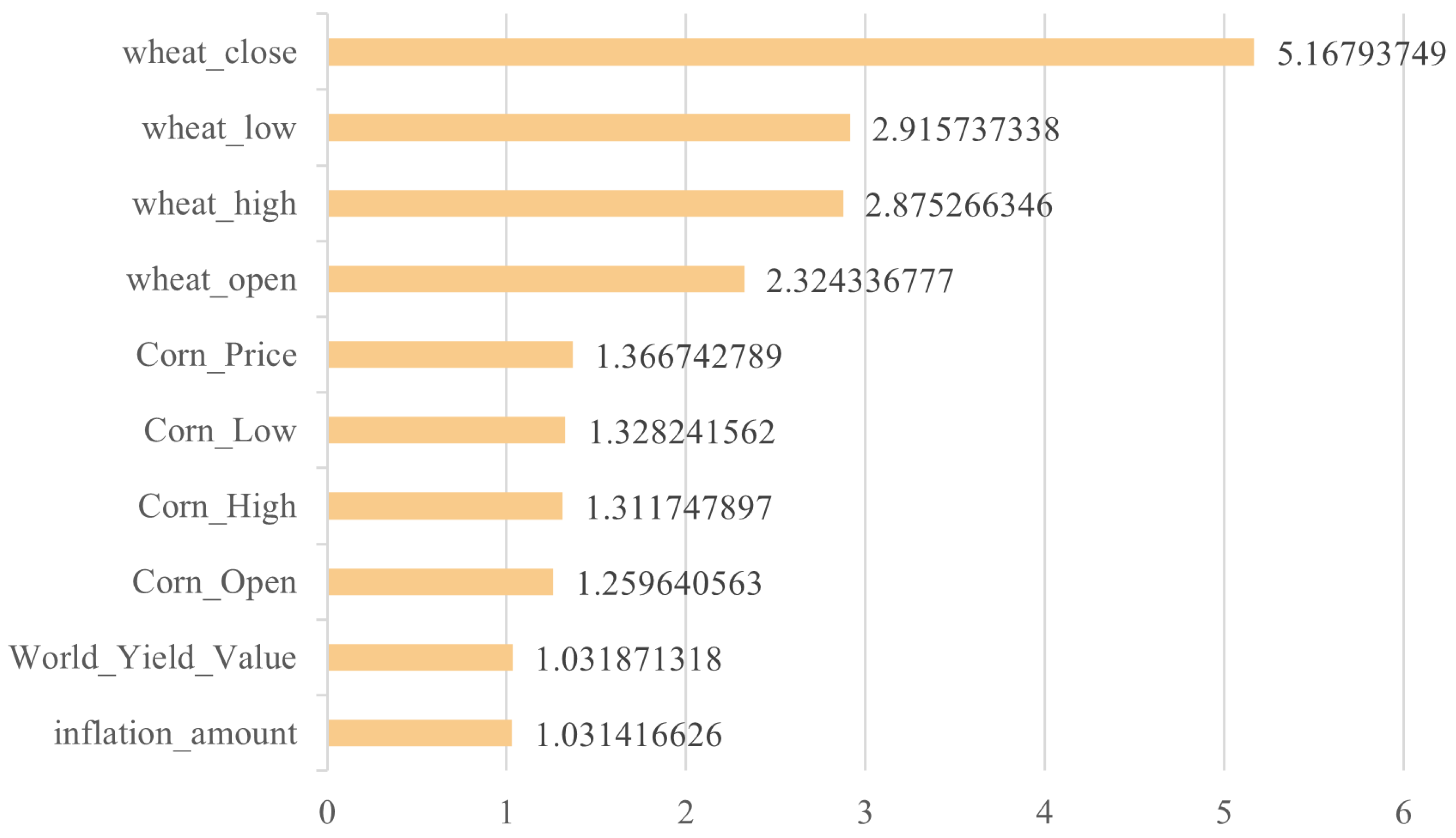
The mutual information value ranking of each feature and the wheat futures price was obtained by the mutual information method in
Section 2.1, as shown in
Figure 5, which shows the mutual information values of each feature with a partial top ranking. Features with low relevance to the target were excluded, and features with higher relevance were selected as the model input to achieve faster training speed and better model performance.
From
Figure 5, it can be found that the mutual information values of different features and wheat futures are arranged in gradient order, and the first four features have a high correlation, which are wheat closing_price, low_price, high_price, and open_price. After the fifth feature, the correlation does not change much, so in this experiment, the first 1, 2, 3, 4, 5, 6, and 7 features were selected as the input for experimental comparison to determine the optimal number of features.
For the top 1, 2, 3, 4, 5, 6, and 7 features selected by the mutual information method as the input of the Bi-DSConvLSTM-Attention model for comparison, the experimental results of various performance evaluation indicators are shown in
Table 3.
The experimental results show that the model had the best performance when the first four features were selected as the input. Therefore, the optimal number of features was four, that is wheat_close, wheat_low, wheat_high, and wheat_open were selected as the input features of the model, which greatly reduced the data dimension and improved the training efficiency of the model.
3.4. Attention Mechanisms’ Analysis
On the basis of the Bi-DSConvLSTM model, a comparative analysis was conducted by adding eight-head attention, four-head attention, two-head attention, self-attention, and no attention. The prediction results are shown in
Table 4.
According to the experiment, it can be seen that the attention mechanism can effectively improve the accuracy of the model. Compared with the self-attention mechanism, although the RMSE, MAE, MAPE, and of the eight-head attention mechanism and the four-head attention mechanism were basically the same for wheat futures prediction, the training time was longer under the same epoch. However, the two-head attention mechanism had a higher error rate. Therefore, in the futures price prediction, this paper chooses the self-attention mechanism.
3.5. The Performance Analysis
Considering computational resources and efficiency, we selected wheat_close, wheat_low, wheat_high, and wheat_open as the input features for the models. We compared the price prediction performance of seven existing models: Bi-ConvLSTM-Attention, LSTM, BiLSTM, LSTM-Attention, TCN-Attention, CNN-BiLSTM-Attention, and BiLSTM-Attention [
36]. The performance of wheat price prediction on the test data set for each model is shown in
Table 5.
The experimental results showed that the Bi-DSConvLSTM-Attention model performed better on various performance evaluation indicators compared with Bi-ConvLSTM-Attention, LSTM, BiLSTM, ConvLSTM, TCN-Attention, CNN-BiLSTM-Attention, and BiLSTM-Attention.
The RMSE experimental results of the Bi-DSConvLSTM-Attention model were 17.50%, 64.27%, 61.73%, 52.46%, 63.15%, 45.59%, and 57.77% higher than those of Bi-ConvLSTM-Attention, LSTM, BiLSTM, ConvLSTM, TCN-Attention, CNN-BiLSTM-Attention, and BiLSTM-Attention, respectively. The MAE experimental results were 21.60%, 71.97%, 70.32%, 55.30%, 67.82%, 57.54%, and 63.48% higher than those of Bi-ConvLSTM-Attention, LSTM, BiLSTM, ConvLSTM, TCN-Attention, CNN-BiLSTM-Attention, and BiLSTM-Attention, respectively. The MAPE experimental results were 25.68%, 72.36%, 71.50%, 56.00%, 70.90%, 58.65%, and 60.71% higher than those of Bi-ConvLSTM-Attention, LSTM, BiLSTM, ConvLSTM, TCN-Attention, CNN-BiLSTM-Attention, and BiLSTM-Attention, respectively. On
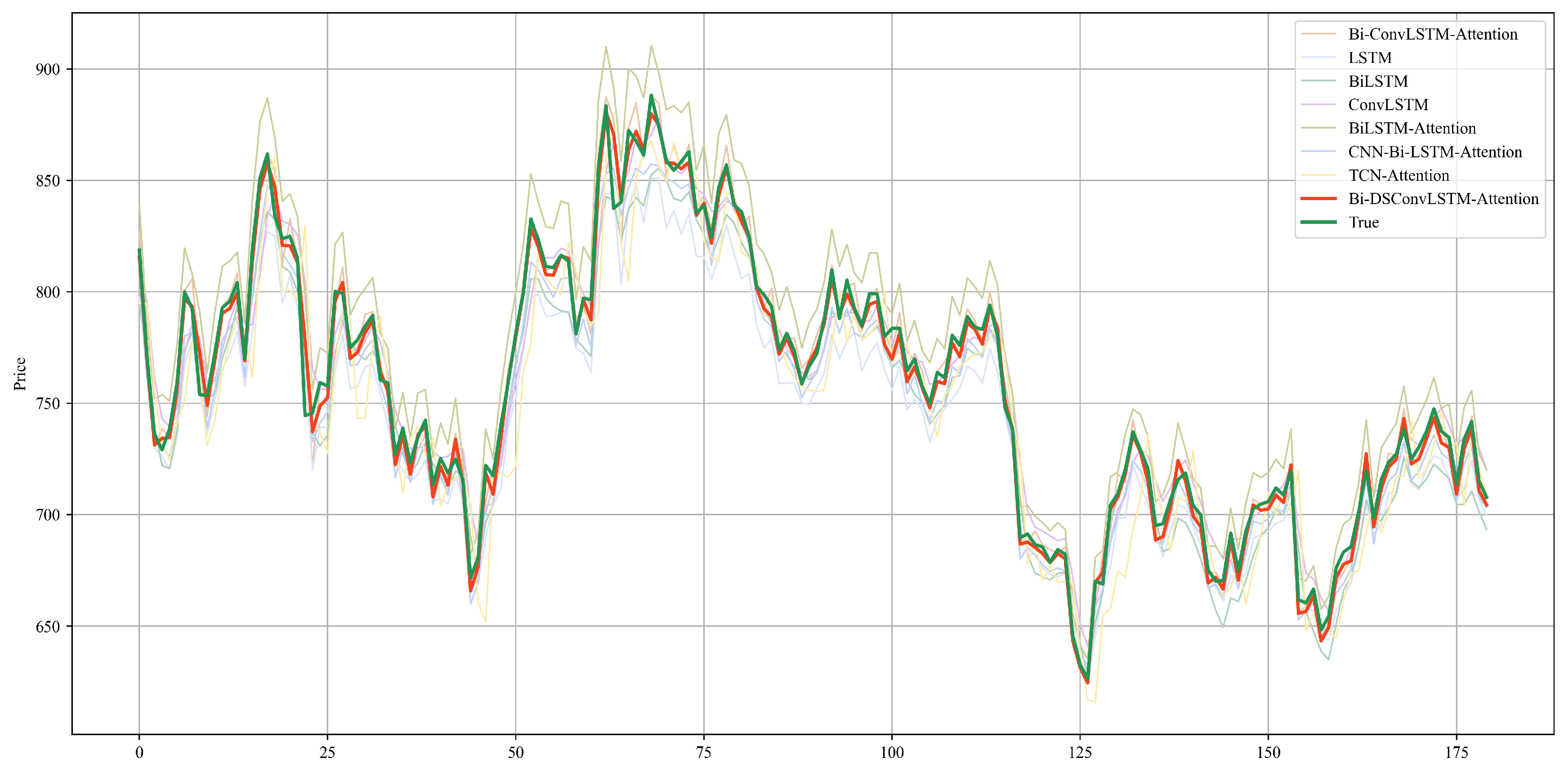
R2, the proposed Bi-DSConvLSTM-Attention model also outperformed the other common models. The prediction results of these models for the futures price of the next 180 days are visualized in
Figure 6.
3.6. Generalization Analysis
In order to verify the universality of Bi-DSConvLSTM-Attention on different grains, this paper also conducts the same experiment test on soybean. The experimental results are shown in
Table 6.
The experimental results showed that the error of Bi-DSConvLSTM-Attention was much lower than that of the commonly used time series prediction models. It was verified that the model has strong generalization ability.
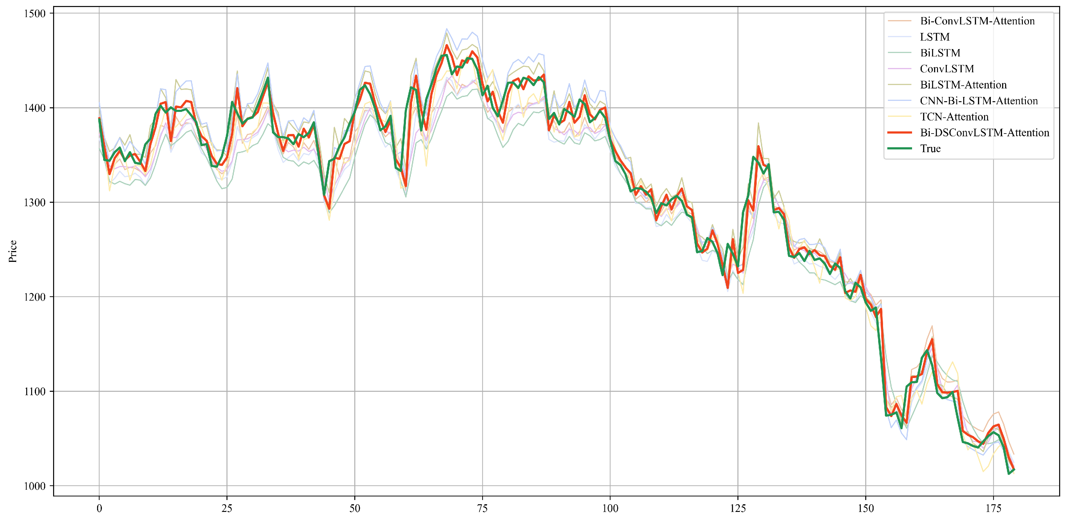
The prediction results of these models, for the futures price of the next 180 days, are visualized in
Figure 7.
3.7. Efficiency Analysis
According to
Section 2.2, DSConvLSTM has fewer parameters than SConvLSTM, so Bi-DSConvLSTM-Attention should have higher efficiency. In this paper, we compared the average time of Bi-DSConvLSTM-Attention and Bi-ConvLSTM-Attention over multiple runs. The experimental results are shown in
Table 7.
The experimental results showed that the use of DSConv can reduce the run time by about 10%, and the number of parameters is reduced by about 25%, so the use of DSConv has a significant efficiency advantage.
3.8. Return Test Analysis
According to the literature [
37], in order to assess whether our model can yield positive returns, we conducted multiple training iterations and calculated the average profit and loss (PNL) to evaluate the outcomes on the test dataset.
The average PNL on the test set was 1.52%.
Since the PNL was positive, holding or selling grain according to the forecast results of our prediction model can obtain positive returns.

