A Two-Echelon Multi-Trip Capacitated Vehicle Routing Problem with Time Windows for Fresh E-Commerce Logistics under Front Warehouse Mode

Abstract

Given the swift expansion of fresh e-commerce, the front warehouse mode can respond quickly and ensure the quality of fresh products. However, the complexity of the supply chain structure under front warehouse mode poses a challenge in reducing logistics costs and improving distribution efficiency while meeting consumers’ immediate delivery demands. Therefore, this paper studies the vehicle routing problem of two-echelon fresh e-commerce under front warehouse mode. Considering trans-shipment time constraints between the two echelons and the characteristics of terminal distribution, this paper initially models the vehicle routing problem for front warehouses as a two-echelon multi-trip capacitated vehicle routing problem with time windows. A mixed-integer linear programming model is subsequently established. To solve the model, a hybrid genetic algorithm integrated with neighborhood search is developed. Matrix coding is employed to merge vehicle selection and route assignment decisions. Simultaneously, neighborhood search is applied to enhance the search capability of algorithms, thereby improving the quality of solutions. Furthermore, the effectiveness and efficiency of the model and algorithm are verified through experiments of varying scales. Finally, comparative strategies and sensitivity analysis highlight the advantages of multi-trip strategies and provide insights into the optimal vehicle capacity limit.

1. Introduction

With the continuous advancements in Internet technology and the rapid expansion of e-commerce, consumer behavior has gradually shifted from offline to online consumption. Fresh e-commerce platforms, emerging as a new consumption channel, have seen a significant increase in user demand. The report [1] indicates that the transaction volume of China’s fresh e-commerce sector has grown substantially, from RMB 195 billion in 2018 to RMB 642.8 billion in 2023. It is forecasted that the transaction volume will ascend to RMB 736.8 billion in 2024.

In addition to the growing demand for fresh products in the e-commerce market, heightened living standards have led to increased consumer expectations regarding the quality of fresh products. The perishable nature of these goods necessitates that cold chain logistics, particularly in urban last-mile delivery, meet elevated standards of efficiency. Moreover, beyond the fundamental need for timeliness in fresh produce delivery, there is a rising expectation among consumers for rapid response capabilities in immediate ordering and delivery systems. These demands have prompted the emergence of the front warehouse mode.

To address the issue of delivery in B2C, the front warehouse mode was first introduced in 2015. This mode represents an emerging storage and distribution mode under the new retail industry, where e-commerce companies establish small-scale warehouses closer to consumers, directly supplied by central warehouses. Upon customer orders, products can be dispatched from the front warehouse nearest to the consumer. The advantages of the front warehouse mode not only include ensuring the timely delivery of fresh produce but also satisfying customer demands for immediate order fulfillment. Additionally, due to its inherent storage capabilities, this mode can accommodate the refrigeration needs required by fresh products. Consequently, the front warehouse mode has increasingly become a prominent trend in new retail.

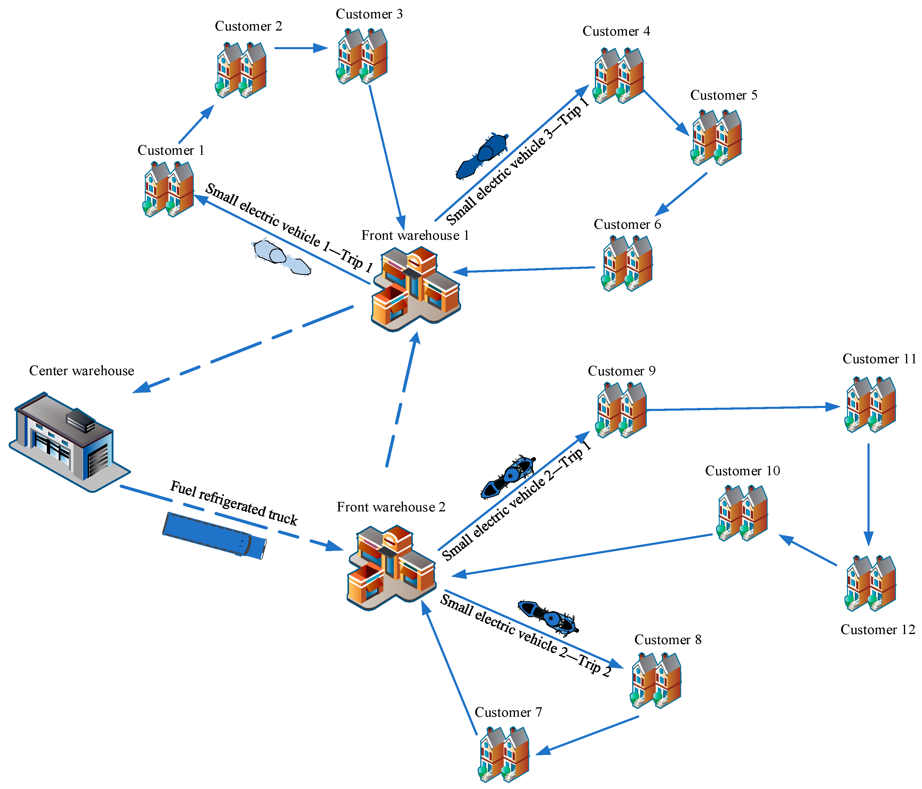
The logistical network of the front warehouse mode is based on a two-echelon supply chain structure of “urban central warehouse–front warehouse–customer”. As shown in Figure 1, fresh products are transported to the front warehouses by fuel refrigerated trucks, and then the products are delivered to customers by small electric vehicles in multiple trips. This new distribution model has been widely used in China’s urban logistics, such as Hema Fresh, Meituan, Dingdong, and so on. Among them, in 2022, there were 1300 front warehouses for Dingdong, and as of May 2024, Hema Fresh set up 360 stores across the country, and it is expected to exceed 400 stores in 2024. However, compared to traditional fresh produce supply chains, the front warehouse mode involves a longer logistics network, higher network costs, and increased complexity in supply chain management. Additionally, to minimize quality degradation and preserve freshness, fresh products require refrigerated storage, leading to logistics costs approximately 130% higher than those for non-perishable products. The key challenge lies in effectively planning delivery routes and allocating personnel and vehicles to meet customer demands while enhancing customer satisfaction and reducing logistics costs.

This paper investigates the two-echelon vehicle routing problem (2E-VRP) in e-commerce logistics under the front warehouse mode. Due to the characteristics of last-mile delivery, such as high frequency, small batch, time sensitivity, and short distances, the 2E-VRP for front warehouses is conceptualized as a two-echelon multi-trip capacitated vehicle routing problem with time windows (2E-MTCVRPTW). The first stage of distribution from the central warehouse to front warehouses, involving large trucks, is conceptualized as a classic vehicle routing problem with time windows (VRPTW). The second stage of distribution between front warehouses and customer points, utilizing small electric vehicles, is defined as a multi-trip capacitated vehicle routing problem with time windows (MTCVRPTW). Taking into account constraints such as trans-shipment synchronization, customer demand time windows, vehicle load, and multi-vehicle coordination, a mixed-integer linear programming (MILP) model is developed with the objective of minimizing the comprehensive transportation costs of vehicles in both stages. The main contributions of this paper are as follows:

(1)

Considering trans-shipment between two echelons and mixed-vehicle fleets across different echelons, this study constructs a 2E-MTCVRPTW model to minimize total logistics costs under the front warehouse mode. This model simultaneously optimizes the two-echelon distribution problem, reducing delivery costs and enhancing service efficiency.

(2)

Research on e-commerce logistics for fresh food primarily focuses on the classic capacitated vehicle routing problem with time windows (CVRPTW). However, in reality, the expansion of fleet size cannot be sustained indefinitely. A multi-trip strategy is adopted for the delivery stage between front warehouses and customers, enhancing fleet resource efficiency and producing vehicle routing solutions that better align with actual operational conditions.

(3)

An improved Genetic Algorithm (GA) combined with neighborhood search is used to solve large-scale problems, proving its effectiveness in optimizing intricate logistics scenarios. A matrix coding method tailored to the problem’s specifics facilitates vehicle selection and route planning. Enhanced by neighborhood search, the algorithm’s search efficiency and solution quality are significantly improved.

The rest of this paper is organized as follows. Section 2 reviews the literature on fresh e-commerce distribution network optimization and identifies potential research gaps. Section 3 describes the logistics routing optimization problem for front warehouses as a 2E-MTCVRPTW, formulated as an MILP model with the objective of minimizing costs. In Section 4, an enhanced hybrid algorithm is developed to solve this NP-Hard problem, incorporating matrix coding and neighborhood search to improve the GA. Section 5 validates the model and algorithm’s effectiveness and feasibility through numerical experiments using real-case scenarios of fresh e-commerce enterprises, including a comparative analysis of multi-trip strategies and sensitivity analysis. The conclusion of this paper is given in Section 6.

2. Literature Review

Currently, there is limited theoretical research on front warehouses, with most of the literature focusing on the business model of front warehouses. The majority of this research is concentrated on strategic-level issues such as facility location. There is scant research on logistical route optimization at the operational level of front warehouses. The analysis of actual logistics operations for front warehouses reveals that they are part of a two-echelon distributed storage system, and their logistics network route optimization represents a 2E-VRP. Furthermore, due to the high frequency of end deliveries in front warehouses, their situation is similar to the multi-trip vehicle routing problem (MTVRP).

2.1. Fresh Products Supply Chain Network

In recent years, numerous scholars have extensively researched the network design optimization problem for fresh products. Ref. [2] developed a model to study distributors’ considerations of quality and quantity for perishable products and producers’ decisions on the optimal wholesale price of perishable products and described the optimal decisions of each party in decentralized and centralized systems. In the research on the strategic and tactical decision making considering cold chain logistics, the perishability of fresh products is taken into account to determine the optimal cold location and distribution (see [3,4]), as well as the optimal inventory decision (see [5,6]). Meanwhile, some scholars have jointly optimized the location and inventory decisions in cold chain logistics and more comprehensively considered the impact of perishability of fresh products on cold chain logistics (see [7,8]).

In addition, there is a lot of research on the operational decision making of fresh products (see [9,10,11]). Ref. [12] considered a multi-commodity perishable food VRP for refrigerated trucks and general-purpose vehicles to maximize the overall level of customer satisfaction, which depends on the freshness of the delivered product. Ref. [13] proposed a time-constrained Eco-routing problem, taking the deterioration process into account when delivering perishables, and established a bi-objective nonlinear model for the Eco-routing problem. Ref. [14] investigated an integrated VRP for perishable foods with storage temperature control and quality requirements.

2.2. The Vehicle Routing Problem under Front Warehouse Mode

The VRP was first studied in [15] to make decisions about the vehicle route of a visiting customer. Over several decades, the classic VRP model has evolved into various complex variants that meet real-world needs [16]. On the basis of classical VRP, the researchers considered the influence of factors such as capacity constraints, multiple depots, multiple products, multiple trips, time windows, time-dependency, and stochastic demand on decision-making. Ref. [17] examined the crowdsourcing-based urban parcel transit distribution system, breaking down the trucking issue into two distinct problems: the winner determination problem and the simultaneous pickup and delivery problem with soft time windows. Ref. [18] studied the VRP for load-dependent drones and formulated a branch-and-price-and-cut algorithm within the Dantzig–Wolfe decomposition framework. Ref. [19] focused on multiple vehicle routing problems under a maximum capacity constraint and no time constraint, comparing three optimization algorithms: intra-route local search, inter-route local search, and tabu search.

Several scholars have conducted research on the logistics network optimization of the front warehouse mode (see [20,21]). Besides optimizing inventory strategies and addressing location issues, some researchers have also studied the immediate delivery aspects of front warehouses. Considering the practical factors affecting the planning of the order execution process, Ref. [22] proposed a mixed-integer programming (MIP) model with the goal of minimizing costs to deal with the integration scheduling of zone picking and VRPTW and proposed a two-stage iterative search algorithm. Ref. [23] considered the practical characteristics such as order segmentation constraints based on product type and quantity and heterogeneous vehicle route constraints and established an integrated optimization model for order segmentation and CVRPTW under the front warehouse mode.

2.3. The Two-Echelon Vehicle Routing Problem

VRPs set within a two-echelon logistics network are collectively termed as 2E-VRPs, representing a variant of the classic VRP (see [24,25]). Refs. [26,27] studied the 2E-CVRP considering environmental factors. Ref. [28] proposed an MILP model of a two-echelon distribution system considering the change in real-time trans-shipment capacity and designed a two-stage heuristic algorithm to solve the problem. Ref. [29] studied the multi-commodity 2E-CVRP with time windows and developed an exact solution approach based on a decomposition scheme. Ref. [30] studied the two-echelon distribution problem of multiple commodities with the goal of minimizing the transportation cost from supplier to customer and presented two sequential solutions based on the collection subproblem and the delivery subproblem in different sequences. Ref. [31] formulated the 2E-VRP with stochastic requirements as an opportunity-constrained stochastic optimization problem and proposed two effective solution methods based on column generation.

Due to the complexity of the 2E-VRP, most scholars use heuristic algorithms to find solutions. Ref. [32] studied the 2E-VRP with simultaneous pickup and delivery, proposed a node-based mathematical model, and proposed a hybrid heuristic algorithm based on variable neighborhood descent and local search to solve the model. Ref. [33] proposed a graph-based fuzzy evolution algorithm to solve the 2E-VRP problem. This method integrates a graph-based fuzzy allocation scheme into the iterative evolutionary learning process to minimize the total cost. Ref. [34] studied the 2E-VRP, where customer points are reachable by synchronized two-echelon fleets, developing an MIP model aimed at optimizing economic, environmental, and social objectives. They employed a large neighborhood search within a heuristic rectangular segmentation to address this problem. Refs. [35,36,37] employed an adaptive large neighborhood search algorithm (ALNS) for the 2E-VRP considering different factors.

2.4. The Multi-Trip Vehicle Routing Problem

Delivery personnel and vehicles can depart from the front warehouse multiple times within a single day to execute deliveries, returning to the warehouse to await subsequent departures until all delivery tasks are completed. Research focused on this operational model addresses the VRP known as the capacitated multi-trip vehicle routing problem (CMTVRP) in [38]. The CMTVRP has recently attracted significant attention due to its frequent application in real-life scenarios such as urban logistics and last-mile delivery. Ref. [39] proposed three meta-heuristic algorithms for the multi-depot multi-trip heterogeneous dial-a-ride problem: improved ALNS, hybrid bee algorithm with simulated annealing, and hybrid bee algorithm with deterministic annealing. Ref. [40] designed two branch-and-price frameworks to solve the multi-trip vehicle routing problem with time windows (MTVRPTW), considering the case of mandatory access to all customers and no duration limit. Ref. [41] established two integer programming models for MTVRPTW, incorporating variable loading times based on service and restricted travel durations. Ref. [42] proposed an exact solution framework based on column generation, column enumeration, and cutting planes to solve large-scale MTVRP. Ref. [43] studied a multi-trip single VRP based on AND-type priority constraints, established three MIP models with the goal of minimizing the cost of total trips, and designed a logic-based benders decomposition algorithm to solve the problem.

There has also been considerable research by scholars on the applications and extensions of the MTVRP. Ref. [44] devised an MTVRP for when customers are in close proximity to each other or when demand is high which uses specific operators designed to solve the problem simultaneously in terms of routing and assignment. Ref. [45] studied a heterogeneous fleet MTVRP considering docking constraints and a realistic objective function and designed a trajectory search heuristic algorithm combining iterative local search, greedy randomized adaptive search procedure, and variable neighborhood descent procedures. Ref. [46] studied a multi-depot MTVRPTW with a release date in a last-mile delivery operation to minimize the total travel time and build an MIP model. In order to solve this problem, a hybrid particle swarm optimization (PSO) algorithm and a hybrid GA were proposed. Ref. [47] studied a time-dependent MTVRPTW considering the travel time and the loading time in the depot simultaneously and developed a hybrid meta-heuristic algorithm to solve the problem. Ref. [48] established an MIP model aimed at minimizing the total time for the joint optimization of heterogeneous CMTVRP coordinated with production scheduling. They designed a memetic algorithm and a simulated annealing algorithm to solve the model.

In summary, extensive research has been conducted on the extended VRP. However, as demonstrated in

Table 1. Summary of related papers.

References	VRP		FW	Factors			Method
	2E	MT		Capacity	MT-V	TW
Ref. [12]				√	√	√	Heuristic algorithm
Ref. [14]				√		√	General variable neighborhood search
Ref. [19]				√			Intra-, inter-route local search, tabu search
Ref. [22]			√			√	Two-stage iterated search
Ref. [23]			√	√	√	√	Branch-price-and-cut
Ref. [28]	√			√	√	√	Two-stage heuristic algorithm
Ref. [29]	√			√		√	Branch-and-price
Ref. [34]	√			√	√	√	Large neighborhood search
Ref. [39]		√		√	√	√	Hybrid meta-heuristic methods
Ref. [41]		√		√		√	Two two-index compact models
Ref. [46]		√		√		√	Hybrid PSO and GA
Ref. [49]		√			√	√	Branch-and-price
Ref. [50]	√	√		√	√	√	Branch-cut-and-price
Ref. [51]	√		√	√		√	Neighborhood structures
This paper	√	√	√	√	√	√	Hybrid GA combining neighborhood search

Notes: (1) 2E represents two-echelon. (2) MT represents multi-trip. (3) FW represents the front warehouse. (4) MT-V represents multi-type vehicles. (5) TW represents time windows.

, most VRP studies focus solely on single-echelon last-mile delivery, with less consideration given to the simultaneous optimization of two-echelon routing schemes. Consequently, there is also limited research on the heterogeneous fleet within the two-echelon system. Moreover, studies on VRP issues under the front warehouse mode of new retail are relatively scarce. Ref. [49] studied the heterogeneous fleet multi-depot MTVRPTW under shared depot resources, in which the travel times of small and large vehicles in a specific area are different. However, they have not considered the two-echelon system, nor have they focused on the front warehouse mode under the new retail context. Ref. [50] considered a 2E-VRP, but not in the front warehouse mode. Ref. [51] studied the VRP of the last-mile delivery service of large household appliances under the front warehouse mode and explored the neighborhood structures with the newly proposed mobile operator in variable neighborhood search and stochastic tabu threshold. However, they did not consider the different types of vehicles within the two-echelon system. This paper addresses the 2E-VRP with different types of vehicles under the front warehouse mode, transforming the last-mile delivery from the front warehouse to customer points into a 2E-MTCVRPTW.

3. Optimization of E-Commerce Logistics Route under the Front Warehouse Mode

Section 3 models the VRP of “urban central warehouse–front warehouse–customer” under the front warehouse mode and obtains two stages of vehicle routing plans. Among them, Section 3.1 describes the problem, and Section 3.2 and Section 3.3 describe the model assumptions and mathematical model of 2E-MTCVRPTW under the front warehouse mode, respectively.

3.1. Problem Description

The e-commerce logistics VRP under the front warehouse mode is demonstrated using the example of Hema Fresh. Hema Fresh is a new retail supermarket in China that offers fresh food and daily necessities. Emphasizing product quality and immediate customer service, it employs a front warehouse mode to provide customers with both online and offline shopping channels. Its rapid expansion has also demonstrated the potential of new retail models. The supply chain network structure is fixed, with customer demands within the delivery radius of a front warehouse being met by that specific warehouse. Orders cannot be placed by customers outside the delivery area, and the delivery ranges of individual front warehouses do not overlap. Transportation from the origin to the central warehouse, generally managed by various suppliers and external to the front warehouse’s logistics system, is excluded from consideration, along with the central warehouse’s storage capacity and cost. As illustrated in Figure 2, this two-echelon network consists of a central warehouse, multiple front warehouses, and various customer points, with known delivery ranges for each front warehouse. Each point in the network, whether a central warehouse, front warehouse, or customer point, is denoted as point i, with the arc between two points represented as $(i,j)$, where the distance A_i,j and transportation time t_i,j of each arc $(i,j)$ are known.

In the two-echelon supply chain network, given the considerable distance between an urban central warehouse and customer points, the use of large freight vehicles for direct deliveries results in high empty load rates, poor timeliness, and elevated transportation costs. Therefore, different vehicles are used for delivery in the two stages, with a front warehouse responsible for unpacking, consolidating, and trans-shipping the goods between the echelons. This paper focuses on the terminal distribution of fresh products at front warehouses; hence, only the online demand from customers for the front warehouse is addressed. Given the premise that customer point demands are known and must be completely satisfied, the central warehouse facilitates the transport of required products to the specified front warehouse via fuel refrigerated trucks in the first stage. Thereafter, the front warehouse arranges for riders to deliver products to customer points within the required time window using small electric vehicles in the second stage, accommodating the characteristics of small batch size, high frequency, and high time sensitivity in the delivery from the front warehouse to customer points.

In the first stage, fuel refrigerated trucks were deployed, incurring transportation costs $C_{i,j}^U$ per unit distance on the arc $(i,j)$ connecting the central and front warehouses. The distribution of this stage occurred once daily, with the cargo load of each truck not exceeding its maximum capacity. Given the impact of the specific arrival times of products at the front warehouses and the delivery time of customer demand on the subsequent delivery’s timeliness, the arrival time at each front warehouse must precede the latest departure time for the first customer demand at that warehouse. Following the system’s optimized routing, trucks completed their delivery tasks and then returned empty to the central warehouse.

In the second stage, small electric vehicles were employed for short-distance transportation, incurring transportation costs $C_{i,j}^F$ per unit distance on the arc $(i,j)$ between the front warehouse and customer points. Time $t_i^N$ was allocated for warehouse staff to engage in picking, packing, and loading activities before distribution could proceed. The cargo load of each electric vehicle driven by the couriers should not exceed the vehicle’s maximum carrying capacity. The classic VRP typically assumes that each vehicle departs once from the origin and visits all demand points before returning. However, this assumption is impractical in real-world logistics operations.

Currently, fresh e-commerce enterprises operating under the front warehouse mode face restrictions due to urban traffic conditions and emission standards within city logistics. The delivery vehicles commonly used are small electric vehicles or other vehicles with low capacity, which are more suitable for delivery tasks characterized by short routes and high frequency. The MTVRP is illustrated in Figure 3.

In the single-trip problem, visiting all customer points requires multiple vehicles, whereas multi-trip delivery can be accomplished with a single vehicle making several round trips to complete all tasks. Given the constraints of limited delivery personnel and vehicles, multi-trip delivery is implemented to enhance vehicle utilization and reduce fixed expenses, including acquisition, maintenance of vehicles, and wages for couriers. Without the consideration of electric vehicle battery capacity limits, delivery staff and vehicles are able to initiate multiple departures from the front warehouse and must arrive within each customer’s requested time window according to a system-planned delivery schedule. Following the completion of all delivery tasks, the resources return to the front warehouse to await subsequent dispatches until the closure of daily operations. Based on this, the MTVRP decision for the two-stage fresh e-commerce distribution network aims to minimize total costs.

3.2. Model Assumptions

The assumptions for the model are as follows:

(1)

The vehicles in the same stage are all of the same type, and the vehicles are traveling at a constant speed.

(2)

The second stage of delivery must start and end at the same front warehouse for each trip.

(3)

There is no time overlap between each trip in the same vehicle.

(4)

Each vehicle provides one service to each customer.

(5)

The total demand in the vehicle’s trip cannot exceed the vehicle’s capacity.

3.3. Mathematical Model

[MILP]

$$\begin{array}{l}Minimize\hspace{1em}Z={\displaystyle \sum _{u\in U}{\displaystyle \sum _{i\in D\cup S}{\displaystyle \sum _{j\in D\cup S}{C}_{i,j}^U}}}{\tau }_{i,j,u}+{\displaystyle \sum _{f\in F}{\displaystyle \sum _{r\in R}{\displaystyle \sum _{i\in S\cup Z}{\displaystyle \sum _{j\in S\cup Z}{C}_{i,j}^F}}}}{\lambda }_{i,j,f,r}\\ \hspace{1em}\hspace{1em}\hspace{1em}\hspace{1em}\hspace{1em}\hspace{1em}+{\displaystyle \sum _{u\in U}{C}^U}{\eta }_u+{\displaystyle \sum _{f\in F}{\displaystyle \sum _{r\in R}{C}^R{\rho }_{f,r}}}+{\displaystyle \sum _{f\in F}{C}^F{\rho }_{f,0}}\end{array}$$

(1)

This is subject to:

$${\displaystyle \sum _{i\in D\cup S,i\ne j}{\tau }_{i,j,u}}-{\displaystyle \sum _{i\in D\cup S,i\ne j}{\tau }_{j,i,u}}=0\hspace{1em}\forall j\in D\cup S,u\in U$$

(2)

$${\displaystyle \sum _{i\in S}{\displaystyle \sum _{j\in D}{\tau }_{i,j,u}}}⩽{\eta }_u\hspace{1em}\forall u\in U$$

(3)

$${\displaystyle \sum _{i\in Z}{d}_i}{y}_{u,i}⩽{\eta }_u{Q}^U\hspace{1em}\forall u\in U$$

(4)

$${\displaystyle \sum _{u\in U}{y}_{u,i}}=1\hspace{1em}\forall i\in Z$$

(5)

$${\displaystyle \sum _{i\in S}{\tau }_{i,j,u}}=1\hspace{1em}\forall j\in D,u\in U$$

(6)

$${\theta }_{u,j}^A⩾{\theta }_{u,i}^A+t_{i,j}+t_i^N-M\left(1-{\tau }_{i,j,u}\right)\hspace{1em}\forall i\in S\cup D,j\in S,i\ne j,u\in U$$

(7)

$$M\left(1-y_{u,l}\right)+{\displaystyle \sum _{j\in D\cup S}{\tau }_{i,j,u}}⩾1\hspace{1em}\forall i\in S,l\in Z_s,u\in U$$

(8)

$$\sum _{f\in F}\sum _{r\in R}{\gamma }_{f,i,r}=1\hspace{1em}\forall i\in Z$$

(9)

$${\displaystyle \sum _{j\in Z\cup S}{\lambda }_{i,j,f,r}}={\displaystyle \sum _{j\in Z\cup S}{\lambda }_{j,i,f,r}}\hspace{1em}\forall i\in Z,f\in F,r\in R$$

(10)

$${\displaystyle \sum _{j\in (S\cup Z_s)}{\lambda }_{j,i,f,r}={\gamma }_{f,i,r}\hspace{1em}\forall i\in Z_s,s\in S,f\in F_s,r\in R}$$

(11)

$${\rho }_{f,r+1}\le {\rho }_{f,r}\hspace{1em}\forall f\in F,r\in R/\left|R\right|$$

(12)

$$\sum _{i\in Z}{\gamma }_{f,i,r}{d}_i\le {\rho }_{f,r}{Q}^F\hspace{1em}\forall f\in F,r\in R$$

(13)

$$\sum _{i\in Z}{\gamma }_{f,i,r}\le {\rho }_{f,r}|Z|\hspace{1em}\forall f\in F,r\in R$$

(14)

$${\theta }_{f,0}^L⩾{\theta }_{u,i}^A\hspace{1em}\forall i\in S,f\in F_s,u\in U$$

(15)

$${\theta }_{f,j,r}\ge \max \left\{{\theta }_{f,i,r},e_i\right\}+t_i^N+t_{i,j}-M\left(1-{\lambda }_{i,j,f,r}\right)\hspace{1em}\forall i,j\in Z,i\ne j,f\in F,r\in R$$

(16)

$${\theta }_{f,r+1}^L\ge {\theta }_{f,r}^B+t_i^N-M\left(1-{\rho }_{f,r+1}\right)\hspace{1em}\forall i\in S,f\in F_s,r\in R\hspace{1em}$$

(17)

$${\theta }_{f,i,r}\le {\gamma }_{f,i,r}{l}_i\hspace{1em}\forall i\in Z,f\in F,r\in R$$

(18)

$${\theta }_{f,r}^B\ge \max \left\{{\theta }_{f,i,r},e_i\right\}+t_i^N+t_{j,i}-M\left(1-{\gamma }_{f,i,r}\right)\hspace{1em}\forall j\in S,i\in Z_S,f\in F_s,r\in R$$

(19)

$${\rho }_{f,r}\in \{0,1\}\hspace{1em}\forall f\in F,r\in R$$

(20)

$${\lambda }_{i,j,f,r}\in \{0,1\}\hspace{1em}\forall i,j\in S\cup Z,i\ne j,f\in F,r\in R$$

(21)

$${\gamma }_{f,i,r}\in \{0,1\}\hspace{1em}\forall i\in Z,f\in F,r\in R$$

(22)

$${\tau }_{i,j,u}\in \{0,1\}\hspace{1em}\forall i,j\in S\cup D,i\ne j,u\in U$$

(23)

$$y_{u,i}\in \{0,1\}\hspace{1em}\forall i\in Z,u\in U$$

(24)

$${\eta }_u\in \{0,1\}\hspace{1em}\forall u\in U$$

(25)

$${\theta }_{u,i}^A⩾0\hspace{1em}\forall i\in S,u\in U$$

(26)

$${\theta }_{f,r}^L,{\theta }_{f,r}^B⩾0\hspace{1em}\forall f\in F,r\in R$$

(27)

$${\theta }_{f,i,r}⩾0\hspace{1em}\forall f\in F,i\in Z,r\in R$$

(28)

The objective of the model is to minimize costs, delineated in Function (1). The first two terms represent the vehicle transportation costs for the first and second stages, respectively. The third term corresponds to the activation cost of fuel refrigerated trucks, the fourth term relates to the total activation cost of trips undertaken by small electric vehicles, and the fifth term refers to the activation cost of small electric vehicles.

For the first stage, the constraints are as follows:

The constraints (2) signify the flow balance in the first stage, where the number of vehicles entering a node must equal the number of vehicles exiting that node. The constraints (3) indicate that a fuel refrigerated truck can choose at most one route. The constraints (4) ensure that the cargo volume allocated to a fuel refrigerated truck does not exceed its transport capacity limit. The constraints (5) stipulate that the product demand at each customer point must be fulfilled by a single fuel refrigerated truck. The constraints (6) dictate that the fuel refrigerated truck will return to the central warehouse upon completing its task. The constraints (7) pertain to the temporal relationship during the travel of the fuel refrigerated truck. The constraints (8) guarantee that if a fuel refrigerated truck is assigned a transportation task, it will deliver the demanded products to the corresponding front warehouse for customer i.

For the second stage, the constraints are as follows:

The constraints (9) dictate that the demand at each customer point can only be met by a single small electric vehicle in one trip. The constraints (10) ensure flow balance in the second stage, where the number of vehicles arriving at a customer point is the same as the number leaving it. The constraints (11) limit the route choices for each small electric vehicle between the front warehouse and the customer point to at most one per trip. The constraints (12) dictate that the (r + 1)^th trip of a vehicle can only occur if the r^th trip has been completed. The constraints (13) ensure that the total load of a small electric vehicle does not exceed its capacity limit. The constraints (14) ensure that small electric vehicle f serves only customers included in the trip r of vehicle f.

The constraints (15) ensure that for the deliveries in the first stage, the arrival time of the fuel refrigerated truck at the front warehouse must be earlier than the departure time of the small electric vehicle starting its first delivery trip from the same warehouse. The constraints (16) delineate the temporal relationship between successive customer points within the same trip of a small electric vehicle during the second stage. The constraints (17) describe the time relationship between consecutive trips for the same small electric vehicle, where it returns to the front warehouse after completing a delivery and departs for the next delivery. The constraints (18) guarantee that the small electric vehicle arrives at the customer point no later than the latest service time requested by the customer. The constraints (19) describe the temporal relationship between the time a small electric vehicle returns to the front warehouse after completing a trip and its visits to customer points during the trip.

Finally, the constraints (20)–(25) are 0–1 variables and the constraints (26)–(28) are non-negative variables.

4. Hybrid Algorithm Based on Genetic Algorithm and Neighborhood Search

This paper focuses on the 2E-MTCVRPTW under the front warehouse mode, which is an NP-Hard problem. For small-scale problems, CPLEX can be directly utilized to solve the problem. However, in scenarios with numerous front warehouses, customer points, vehicles, and trips, the solution space expands exponentially. This expansion leads to a substantial growth in the number of binary variables during the computation process. Consequently, this complexity hinders the ability of CPLEX to find the optimal solution within a reasonable time. On the other hand, the GA exhibits strong global search capabilities, rapid convergence, and high stability, making it more effective in solving complex VRP issues. Furthermore, neighborhood search can yield higher-quality approximate solutions. Therefore, this paper designs a hybrid algorithm based on the GA and neighborhood search, tailored to the characteristics of the MTVRP.

4.1. Matrix Encoding and Decoding

In the 2E-MTCVRPTW under the front warehouse mode investigated in this paper, the problem within the second-echelon logistic network is categorized as an MTCVRP issue. Utilizing real-number or sequence encoding methods from the classical VRPTW problem can lead to inconsistencies in encoding length, which hinders subsequent genetic operations like crossover and mutation. Therefore, to enhance the algorithm’s solving efficiency, matrix encoding is employed to directly encode feasible solutions within the solution space for chromosome construction. Initially, all points are numbered, with separate designations for front warehouses and customer points.

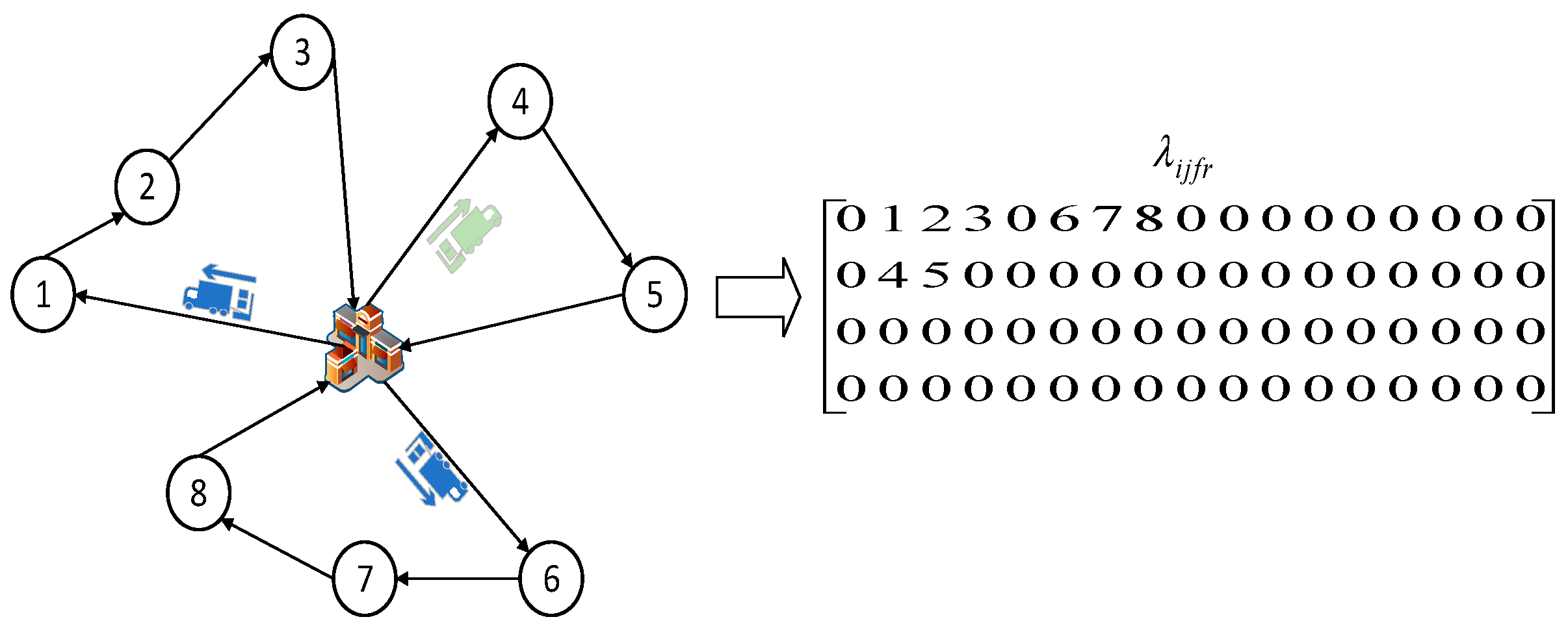
The matrix decoding method employed in this paper is illustrated in Figure 4, taking the structure of one front warehouse and eight customer points as an example. The front warehouse is labeled as 0, and the customer points are numbered {1, 2, …, 8} accordingly. In the matrix, the n^th row corresponds to the route plan for multiple trips made by the n^th vehicle from that front warehouse. Decoding the matrix yields the decision variables ${\lambda }_{0,1,1,1}={\lambda }_{1,2,1,1}={\lambda }_{2,3,1,1}={\lambda }_{3,0,1,1}={\lambda }_{0,6,1,2}={\lambda }_{6,7,1,2}={\lambda }_{7,8,1,2}={\lambda }_{8,0,1,2}=1$, indicating that vehicle 1 is assigned tasks for two trips. It initially departs from the front warehouse to serve customer point 1, then proceeds to customer point 2, followed by a service trip to customer point 3 before returning to the front warehouse. The vehicle awaits its next scheduled departure to commence the second trip, serving customer point 6, followed by customer points 7 and 8, before returning to the front warehouse. This paper integrates vehicle selection and multi-trip route selection through matrix coding. After generating the initial population, infeasible solutions are eliminated based on the sorting of customer points’ time windows and constraints.

4.2. Fitness Function

The fitness function for the problem is designed by the objectives of our problem. Generally, for maximization problems, the objective function corresponds to the fitness function, where a higher fitness function value indicates a greater objective function value and a better feasible solution. Since the objective function in this paper is the total cost of route planning, the fitness function value f_i in the algorithm is set as the reciprocal of the objective function. Thus, a lower cost implies a higher fitness function value, indicating a superior quality of the feasible solution.

$$f_i=1/Z_i,\hspace{1em}\forall i\in \left\{1,2,3,\dots \right\}$$

(29)

4.3. Roulette Wheel Selection and Elitist Preservation

The roulette wheel selection strategy probabilistically selects individuals to form the offspring population. The probability of each individual being selected for the next generation is calculated based on its fitness, with the selection likelihood being directly proportional to the fitness function value. Given that this paper addresses a cost minimization problem, the fitness function has been transformed according to the objective function, converting the issue into a maximization problem. Consequently, the probability of an individual being selected to constitute the offspring population remains in direct proportion to its fitness function value. The higher the proportion of an individual’s fitness function value in the total population fitness, the greater the probability of its selection. The roulette wheel selection strategy facilitates the inheritance of superior individuals into the offspring population, while the generation of random numbers for selection helps maintain population diversity.

Additionally, to prevent the loss of the current population’s optimal individuals in the subsequent generation, which could hinder the GA from converging to the global optimum, an elitism preservation strategy is implemented. This strategy entails retaining the individual with the highest fitness in the current population from undergoing genetic operations such as crossover and mutation. Instead, this elite individual replaces the one with lower fitness in the current generation that resulted from these genetic operations.

4.4. Single-Point Crossover

Crossover involves exchanging segments of genetic material between two parent chromosomes to create new offspring, thus improving individual genes, enhancing population diversity, and increasing the global search capability of the algorithm to prevent entrapment in local optima. The probability of crossover is a crucial factor influencing the generation of superior offspring. This probability p_c determines whether an individual will undergo crossover. In this paper, single-point crossover is employed to perform crossover operations on individuals, and the crossover probability is set at p_c = 0.8.

As illustrated in Figure 5, initially, it is necessary to determine the crossover point coordinates (a, b), where a represents the row crossover point and b represents the column crossover point. Assuming individual X₁ utilizes m₁ vehicles and individual X₂ uses m₂ vehicles, the random integer a should be specified as $[1,\min (m_1,m_2)]$. After determining a, we identify the non-zero columns in the a^th row in matrices X₁ and X₂. The smallest column coordinate value among these becomes the upper limit for the random integer b, with 1 as the lower limit. X₁ has the encoding sequence $\{1,2,3,4,5,6,7,8\}$, and X₂ has the encoding sequence $\{3,5,8,6,2,7,1,4\}$. Figure 5 exemplifies using (2, 2) as the coordinate for the crossover point. The gene sequence $\{1,2,3,4,5\}$ before the crossover point in individual X₁ is retained. First, the gene positions $\{7,8\}$ are deleted, and then the gene sequence $\{8,7\}$ in individual X₂ is reinserted to form the new solution X′₁ after the crossover point.

4.5. Neighborhood Search

The mutation operation using real number encoding in the traditional VRP is not suitable for matrix coding. Neighborhood search is a classic optimization algorithm for the VRPTW. Therefore, this paper employs neighborhood search as a substitute for the mutation operation in the GA to enhance both the global and local search capabilities, thereby improving the quality of solutions.

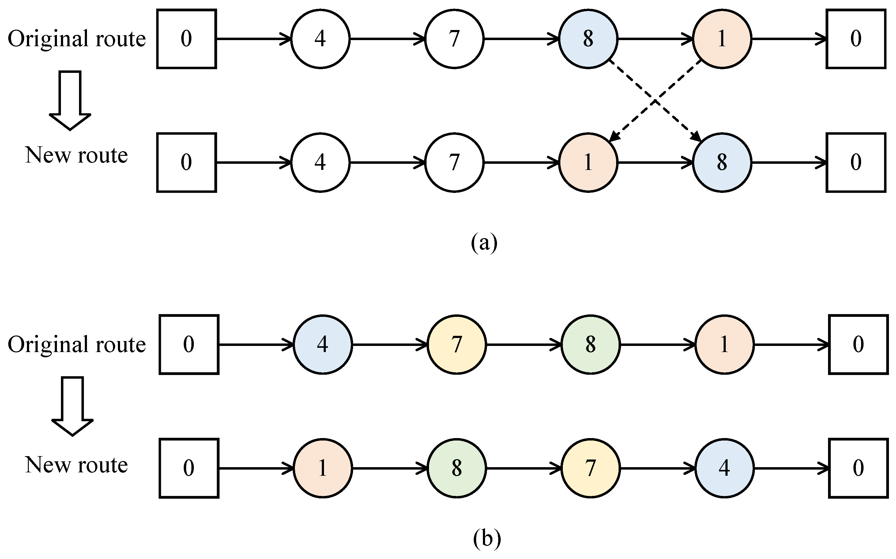
The neighborhood search operator is the core of neighborhood search, and the design of the neighborhood search operator determines the size of the neighborhood range, which is a key factor affecting the quality of the solution. This paper employs neighborhood search operators corresponding to two types of neighborhood structures, reverse and swap variation, to generate new routes, as shown in Figure 6.

Swap variation involves randomly selecting two points on the same segment of a trip’s route. By removing these points, swapping their order, and then reinserting them, a new path can be generated. Reverse variation involves randomly selecting two non-adjacent points, swapping their positions, and then reversing the order of all points between them.

4.6. Process of Hybrid Genetic Algorithm

Due to the increased complexity of solving the MTVRP from the front warehouse to customer points, this paper employs a hybrid GA combining neighborhood search for this stage. Once the corresponding route plan is derived, the total distribution volume for each front warehouse and the earliest departure time for the small electric vehicles can be determined. Consequently, the delivery stage from the central warehouse to the front warehouses can be solved using CPLEX. Following this solution strategy, the complete hybrid GA process (Algorithm 1) for the e-commerce logistics route optimization under the front warehouse mode is as follows:

Algorithm 1: Hybrid genetic algorithm procedure.

1:  INPUT: initial population P(t), maximal iteration τmax: //Initialization 2:  SET τt, fpbest and fgbest, fitness function fi, the population number count, maximum population size L, crossover probability pc; 3:  Generate N particles, and calculate the fitness function fi: //Generate the initial particles 4:    While τt < τmax 5:       Initialize a new population P1(t) and population number Count1 6:          While Count1 < L 7:            Randomly generated for |R| genes and RE, RE$\in$[0,1]: 8:            Roulette operator selection according to RE, update genes to a new P1(t) 9:          End while 10:         Initialize a new population P2(t) and population number Count2 11:         While Count2 < L 12:            Randomly generated M, N$\in$[0, L − 1], p$\in$[0,1] 13:            IF p < pc, then 14:               Genes at M and N cross at a single point to form new genes 15:               The fitness value of the new gene is calculated, and the best gene is put into the new population P2(t) 16:           End if 17:         End while 18:        Initialize a new population P3(t) and population number Count3 19:         While Count3 < L 20:          Swap and reverse variation solves for the new fitness value fi: 21:          IF fi < fpbest, then 22:            Putting new genes into a new P3(t) 23:            Update fpbest, fgbest 24:          End if 25:         End while 26:  End while 27:  OUTPUT: fgbest

5. Numerical Experiments

In this paper, the network layout of the front warehouse of Hema Fresh, a fresh food e-commerce company in Shanghai, China, was studied, and the numerical experiment was carried out in Pudong New District (Area 1). For the sake of transportation convenience, the urban central warehouse of the enterprise is located near the Shanghai Hongqiao Transportation Hub, while the front warehouses are predominantly established in residential and commercial areas across various districts. This section demonstrates the efficiency of the algorithm through experiments of varying scales and validates the model’s effectiveness via comparative analysis of multiple routing strategies. Lastly, the influence of vehicle capacity constraints on the route optimization solution is examined. The algorithm was implemented in C# using CPLEX 12.6.2, and all numerical experiments were conducted on a computer with an AMD Ryzen 7 processor (Developed by AMD, Inc., Santa Clara, CA, USA) running at 2.90 GHz and 16 GB memory.

5.1. Parameter Settings

Incorporating the road traffic network of Shanghai, we obtained the geographical coordinates of the front warehouses and customer points within the delivery range in Area 1 from the map. The latitude and longitude coordinates of the urban central warehouse and select front warehouses in Area 1 are presented in

Table A1. Coordinates of urban central warehouse and front warehouses in Shanghai.

ID of Warehouse	Coordinate		Time Table
	X	Y	Earliest	Latest
${\mathrm{D}}_0$	121.380200	31.187680	0:00	23:59
${\mathrm{S}}_1$	121.584300	31.263860	9:00	22:00
${\mathrm{S}}_2$	121.609800	31.211010	9:00	22:00
${\mathrm{S}}_3$	121.528300	31.185690	9:00	22:00
${\mathrm{S}}_4$	121.659600	31.218090	9:00	22:00
${\mathrm{S}}_5$	121.533200	31.148440	9:00	22:00
${\mathrm{S}}_6$	121.521400	31.232790	9:00	22:00
${\mathrm{S}}_7$	121.498600	31.179540	7:30	22:00
${\mathrm{S}}_8$	121.616800	31.287740	8:00	21:30
${\mathrm{S}}_9$	121.703820	31.204106	8:00	22:00
${\mathrm{S}}_{10}$	121.598029	31.301588	8:30	22:00

of Appendix A. This paper sets the delivery range for the studied front warehouses to within 5 km. Within this range, several residential communities are randomly selected as delivery customer points. For instance, 30 customer points near S₁ are illustrated in

Table A2. The coordinates of residential areas within the coverage area of the front warehouse S₁.

ID of Customer	Coordinate		ID of Customer	Coordinate
	X	Y		X	Y
${\mathrm{C}}_1$	121.588960	31.266140	${\mathrm{C}}_{16}$	121.577475	31.253750
${\mathrm{C}}_2$	121.579582	31.266665	${\mathrm{C}}_{17}$	121.570415	31.260919
${\mathrm{C}}_3$	121.587685	31.264419	${\mathrm{C}}_{18}$	121.572526	31.263736
${\mathrm{C}}_4$	121.590379	31.258894	${\mathrm{C}}_{19}$	121.575876	31.264986
${\mathrm{C}}_5$	121.589355	31.257582	${\mathrm{C}}_{20}$	121.574071	31.264199
${\mathrm{C}}_6$	121.587935	31.253305	${\mathrm{C}}_{21}$	121.591436	31.262757
${\mathrm{C}}_7$	121.589409	31.252581	${\mathrm{C}}_{22}$	121.593420	31.257694
${\mathrm{C}}_8$	121.581037	31.264450	${\mathrm{C}}_{23}$	121.592342	31.248950
${\mathrm{C}}_9$	121.581194	31.258932	${\mathrm{C}}_{24}$	121.583521	31.244110
${\mathrm{C}}_{10}$	121.599080	31.259508	${\mathrm{C}}_{25}$	121.585596	31.241524
${\mathrm{C}}_{11}$	121.579214	31.259557	${\mathrm{C}}_{26}$	121.582443	31.240297
${\mathrm{C}}_{12}$	121.575279	31.258230	${\mathrm{C}}_{27}$	121.580494	31.243014
${\mathrm{C}}_{13}$	121.571322	31.257624	${\mathrm{C}}_{28}$	121.575436	31.245384
${\mathrm{C}}_{14}$	121.570100	31.258990	${\mathrm{C}}_{29}$	121.575724	31.247537
${\mathrm{C}}_{15}$	121.572274	31.253943	${\mathrm{C}}_{30}$	121.573056	31.249227

of Appendix A.

Due to urban road planning and vehicle travel restrictions, the straight-line distance used in the VRP does not reflect the actual driving distance, which is typically longer. In the context of deliveries between front warehouses and customer points, where distances are shorter, this error cannot be overlooked. This paper utilizes map data and latitude–longitude coordinates of points to calculate the actual driving distances between points, forming a symmetric matrix used as the distance parameter. The distance parameters between the central warehouse and the front warehouses are shown in

Table A3. The matrix of distance parameters between the central warehouse and the 10 front warehouses.

Distance Matrix	${\mathbf{D}}_0$	${\mathbf{S}}_1$	${\mathbf{S}}_2$	${\mathbf{S}}_3$	${\mathbf{S}}_4$	${\mathbf{S}}_5$	${\mathbf{S}}_6$	${\mathbf{S}}_7$	${\mathbf{S}}_8$	${\mathbf{S}}_9$	${\mathbf{S}}_{10}$
${\mathrm{D}}_0$	0	3400	500	3000	4600	9500	6700	9800	3100	6800	9500
${\mathrm{S}}_1$	3400	0	7600	1800	900	2700	7300	4600	5600	7000	5400
${\mathrm{S}}_2$	500	7600	0	2000	6600	3300	2700	4500	9600	3000	2100
${\mathrm{S}}_3$	3000	1800	2000	0	6000	5200	6900	3600	5800	800	6400
${\mathrm{S}}_4$	4600	900	6600	6000	0	8700	8500	400	2900	6000	8300
${\mathrm{S}}_5$	9500	2700	3300	5200	8700	0	600	5900	2800	1300	6500
${\mathrm{S}}_6$	6700	7300	2700	6900	8500	600	0	7300	4000	3800	3200
${\mathrm{S}}_7$	9800	4600	4500	3600	400	5900	7300	0	8700	2900	9300
${\mathrm{S}}_8$	3100	5600	9600	5800	2900	2800	4000	8700	0	8900	3500
${\mathrm{S}}_9$	6800	7000	3000	800	6000	1300	3800	2900	8900	0	4200
${\mathrm{S}}_{10}$	9500	5400	2100	6400	8300	6500	3200	9300	3500	4200	0

of Appendix A, and the distance parameter matrices between the front warehouses and customer points are also obtained.

Additionally, based on real-world conditions, the specific performance parameters for the two types of vehicles are set. For the first stage, fuel refrigerated trucks have a specified travel speed $V_1=50\mathrm{km}/\mathrm{h}$, a maximum vehicle capacity $Q^U=400$ L, and a fixed activation cost $C^u=200$. In the second stage, small electric vehicles have a designated travel speed $V_2=20\mathrm{km}/\mathrm{h}$, a maximum vehicle capacity $Q^F=10$ L, a fixed activation cost $C^f=100$, and a per-trip activation cost $C^r=30$. Consumer demand is randomly generated within a specified range [1, 10]. Given current fuel and electricity prices, the transportation costs for fuel refrigerated trucks and small electric vehicles are $C_{i,j}^U=3\ast A_{i,j}$ and $C_{i,j}^F=0.15\ast A_{i,j}$, respectively. In the first stage, there are 5 fuel refrigerated trucks for the delivery task from the central warehouse to the front warehouses. In the second stage, the fleet size of small electric vehicles for each front warehouse is 10, with a maximum of 5 trips per vehicle.

5.2. Experimental Results of Different Scales

To validate the solution efficiency of the hybrid GA, we designed small-, medium-, and large-scale instances. The ID of each instance denotes the number of urban central warehouses, front warehouses, and customer points, for example, 1-2-4 indicates one urban central warehouse, two front warehouses, and four customer points in this distribution network. The maximum computational iteration time for CPLEX is limited to one hour (3600 s), and the iteration threshold for the heuristic algorithm is set at 500. Calculations are performed for the three mentioned scales to compare the results of the improved GA with the exact solutions from CPLEX and the solutions of the standard GA, as detailed in

Table 2. The experimental results for small-, medium-, and large-scale instances.

Scales	ID of Instance	CPLEX		GA			Improved GA
		OBJ	T (s)	OBJGA *	T * (s)	GAP1	OBJIGA *	T * (s)	GAP2
Small	1-2-4	527.83	0.79	527.83	0.07	0.00%	527.83	0.09	0.00%
	1-3-9	757.45	2.46	757.45	0.41	0.00%	757.45	0.52	0.00%
	1-3-12	819.21	2.98	819.21	0.77	0.00%	819.21	0.71	0.00%
	1-3-15	854.09	4.72	854.09	1.12	0.00%	854.09	1.32	0.00%
	1-5-25	1290.34	10.13	1290.34	0.93	0.00%	1290.34	2.98	0.00%
	1-5-30	1458.27	18.43	1477.02	2.56	1.29%	1468.97	2.82	0.73%
	1-5-40	1825.31	35.96	1876.35	7.89	2.80%	1860.09	9.05	1.91%
Medium	1-6-48	2220.6	46.82	2260.87	7.65	1.81%	2239.56	10.34	0.85%
	1-6-54	2596.78	133.56	2659.42	30.42	2.41%	2641.71	26.98	1.73%
	1-7-63	2772.57	385.79	2871.39	62.58	3.56%	2850.57	73.91	2.81%
	1-8-80	3702.66	692.43	3892.94	102.73	5.14%	3789.62	124.35	2.35%
	1-10-100	-	>3600	4508.33	199.45	-	4261.81	214.07	-
	1-10-120	-	>3600	5004.21	292.04	-	4919.58	298.93	-
	1-10-150	-	>3600	5579.72	379.45	-	5242.44	394.25	-
Large	1-10-170	-	>3600	5972.48	470.91	-	5730.37	486.53	-
	1-10-200	-	>3600	7217.09	522.34	-	6805.31	559.13	-
	1-10-220	-	>3600	8143.75	695.48	-	7729.03	703.57	-
	1-10-240	-	>3600	9243.2	767.32	-	8647.16	782.46	-
	1-10-260	-	>3600	9856.96	859.43	-	9166.86	889.27	-
	1-10-280	-	>3600	10,327.31	983.22	-	9377.89	1019.49	-
	1-10-300	-	>3600	10,879.65	1012.54	-	9860.32	1085.67	-

Notes: (1) OBJ represents objective values. (2) T (s) represents the computation time (s). (3) ‘*’ represents the average value obtained after 5 runs. (4) GAP₁ represents the difference in objective between the GA and CPLEX, and GAP₁ is calculated by (OBJ_GA − OBJ_CPLEX)/OBJ_CPLEX. (5) GAP₂ represents the difference in objective between the improved GA and CPLEX, and GAP₂ is calculated by: (OBJ_IGA − OBJ_CPLEX)/OBJ_CPLEX. (6) >3600 indicates that the computation time is more than 1 h and the optimal solution cannot be found. (7) - represents that the value cannot be calculated.

.

From Table 2, it is observable that CPLEX can directly compute the corresponding results, achieving exact solutions when the number of delivery customer points is relatively low. However, as the scale of customer points and front warehouses increases, the solution space expands, resulting in longer computation times. For medium- and large-scale instances with customer points exceeding 80, CPLEX fails to derive the optimal solution within one hour. Conversely, the GA and improved GA can produce superior solutions within a reasonable time for larger-scale instances.

In terms of solution quality, for small- to medium-scale instances, the GA could find the feasible solutions with a minimal gap value relative to the exact solutions of CPLEX in a shorter time. However, as the scale increased, the quality of solutions obtained by the GA gradually decreased. The improved GA, incorporating a neighborhood search, did not exhibit a reduction in computation time compared to the GA. Nonetheless, it achieved solutions with a smaller GAP value compared to the exact solutions calculated by CPLEX, thereby affirming the solution quality and efficiency of the improved GA.

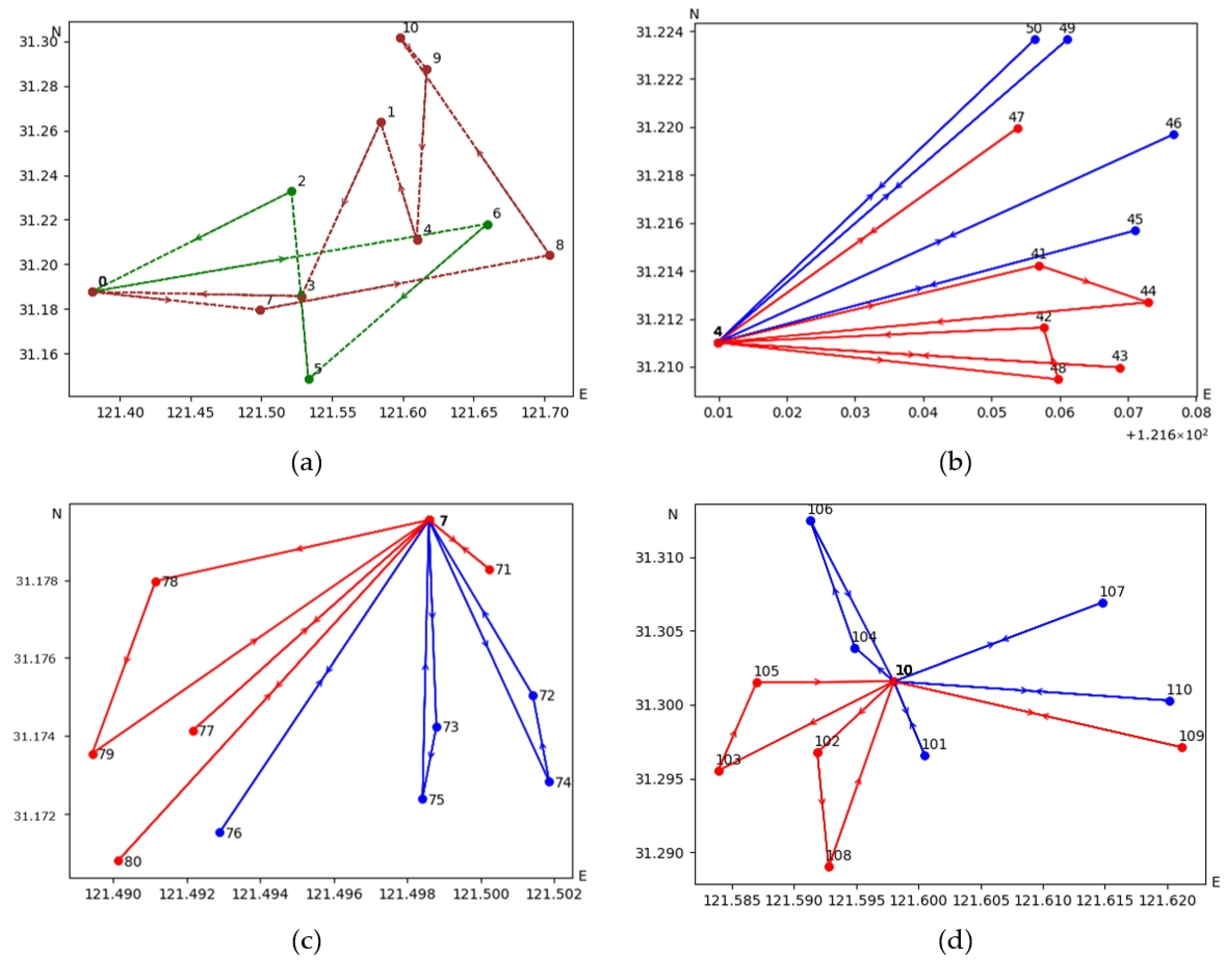
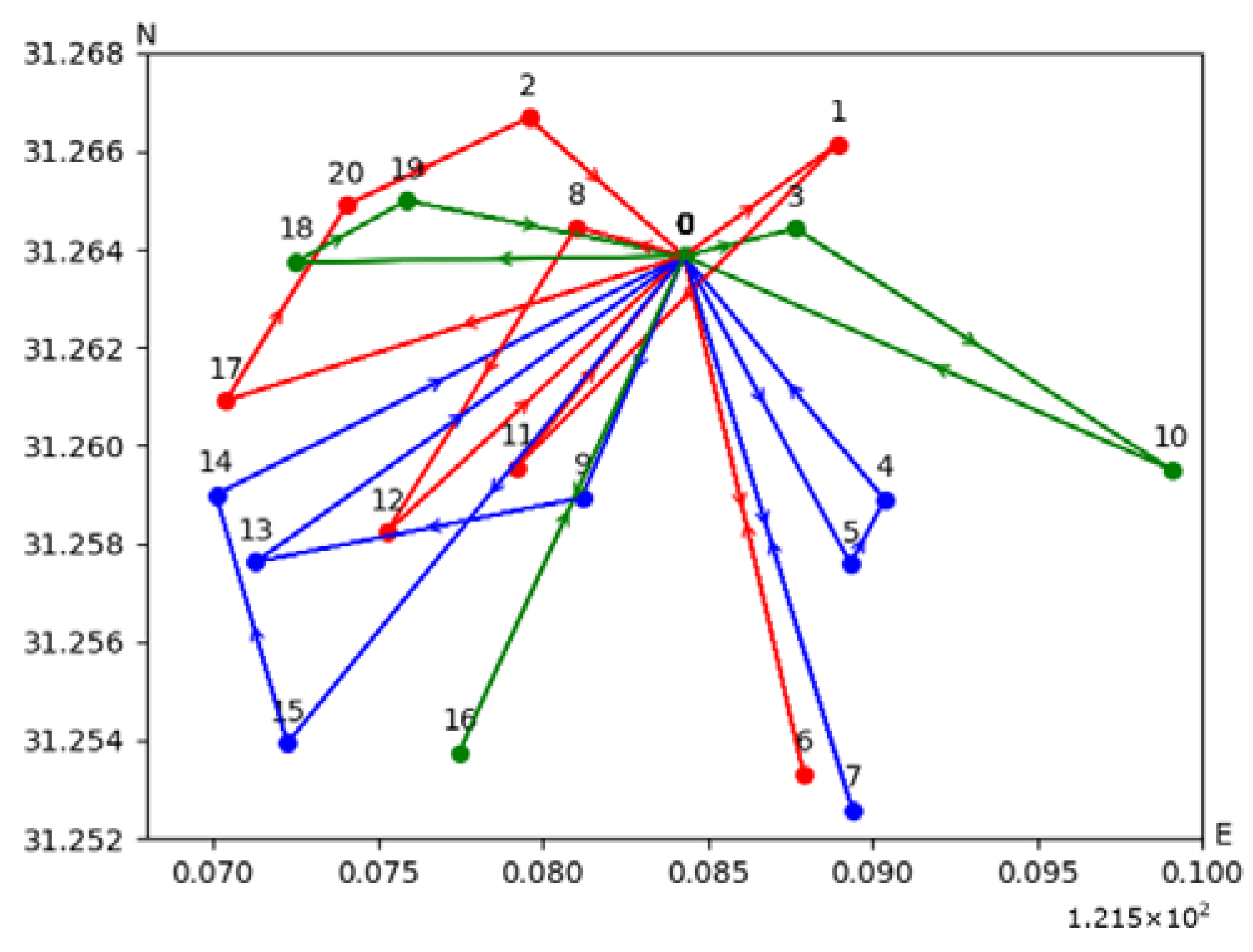
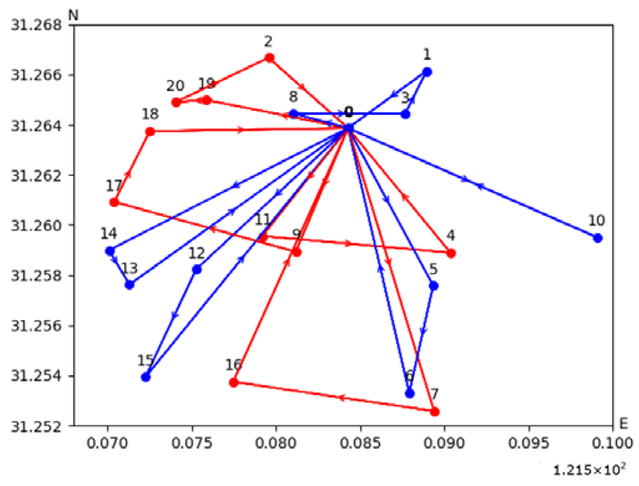
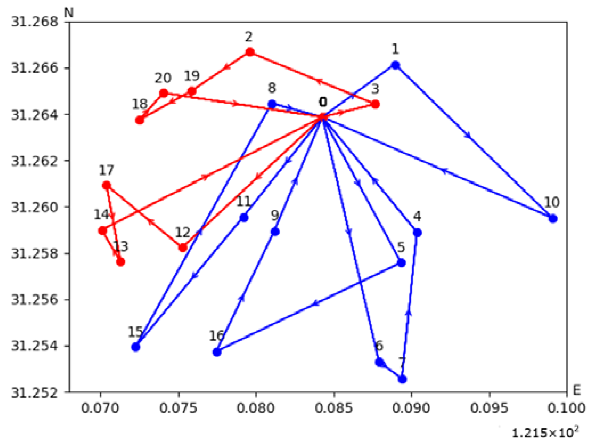
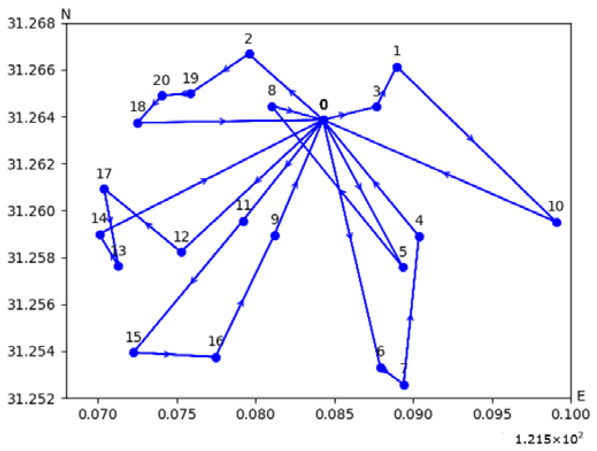
Figure 7 depicts the distribution routes derived from the model proposed in this paper for the 1-10-100 instance. Figure 7a depicts the distribution routes from the central warehouse to the front warehouses in the first stage. Figure 7b–d present the distribution routes from the front warehouses to customer points in the second stage, specifically illustrating the delivery strategies for front warehouses 4, 7, and 10, respectively. The horizontal and vertical coordinates represent the geographical longitude and latitude of the points. In the diagrams, different colors are used to represent distinct vehicles, each capable of conducting multiple trips. In addition,

Table 3. The times in which small electric vehicles visit the customers in front warehouses 4 and 7.

Front Warehouse	Vehicles	Trips	Customer Visit Order	Customer Visit Time
S4	1	1	4-→46→4	9:13
		2	4→49→4	9:40
		3	4→45→4	10:06
		4	4→50→4	10:31
	2	1	4→48→42→4	9:09–9:12
		2	4→43→4	9:33
		3	4→41→44→4	10:07–10:11
		4	4→47→4	10:33
S7	1	1	7→76→7	9:10
		2	7→74→72→7	9:37–9:40
		3	7→73→75→7	10:07–10:10
	2	1	7→78→79→7	9:07–9:13
		2	7→77→7	9:33
		3	7→80→7	10:13
		4	7→71→7	10:33

gives the arrival times of vehicles visiting their customers in front warehouses 4 and 7. The vehicle visits the customer within the time window specified by the customer in the order of the trip.

5.3. Comparative Analysis of Multi-Trip Strategies

To analyze the efficacy of the multi-trip strategy presented in this paper, a comparative analysis with the vehicle routing results under a single-trip strategy is conducted. The front warehouse S₁ and its customer points are selected, with the demand at customer points randomly generated from the range [1, 20]. Reflecting realistic scenarios, customer-available time slots are typically set at one-hour intervals. This experiment specifies that the earliest time window requested by customers is randomly generated at an integral hour between 8:00 and 11:00, with the latest acceptable delivery time being one hour later. For example, the time window for customer point 1 is [8:00, 9:00]. All other parameters remained consistent with the aforementioned numerical experiments.

The experiment constructs three cases, each depicting a supply chain model where a front warehouse supplies various customer points, designed to meet the demands of 10, 15, and 20 customer points, labeled as case numbers 1–10, 1–15, and 1–20, respectively. As the objective function aims to minimize the total cost, the initiation of vehicle dispatches increases the vehicle activation cost. Therefore, the actual number of vehicles used does not necessarily reach the maximum quantity. The fleet size for both strategies is set at 20 vehicles, with a maximum of 5 trips allowed for the multi-trip strategy and a single trip for the single-trip strategy. The comparative results of the multi-trip and single-trip strategies are presented in

Table 4. A comparison of the results of the multi-trip strategy and the single-trip strategy.

Instance	The Single-Trip Strategy				The Multi-Trip Strategy
	Activation Costs	Trip Costs	Number of Vehicles	Number of Trips	Activation Costs	Trip Costs	Number of Vehicles	Number of Trips
1-10	700	210	7	7	100	180	1	6
1-15	800	240	8	8	200	240	2	8
1-20	1300	390	13	13	400	390	4	13

.

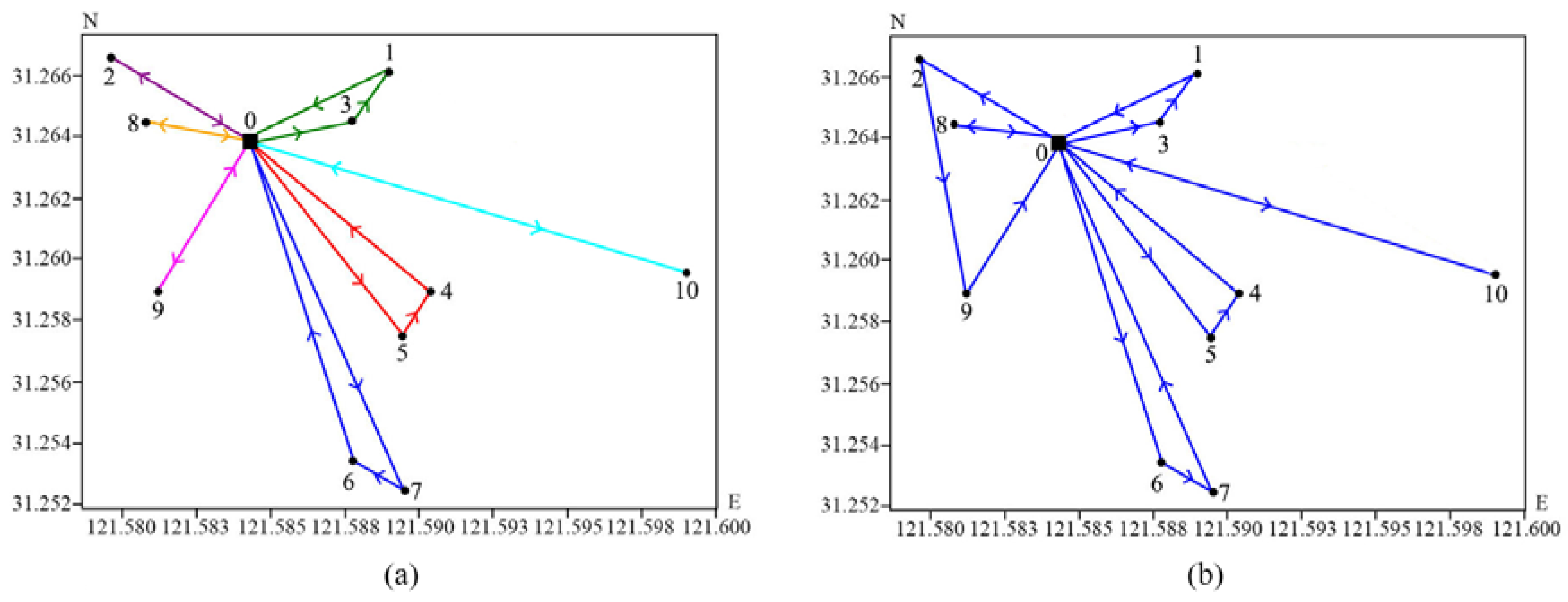
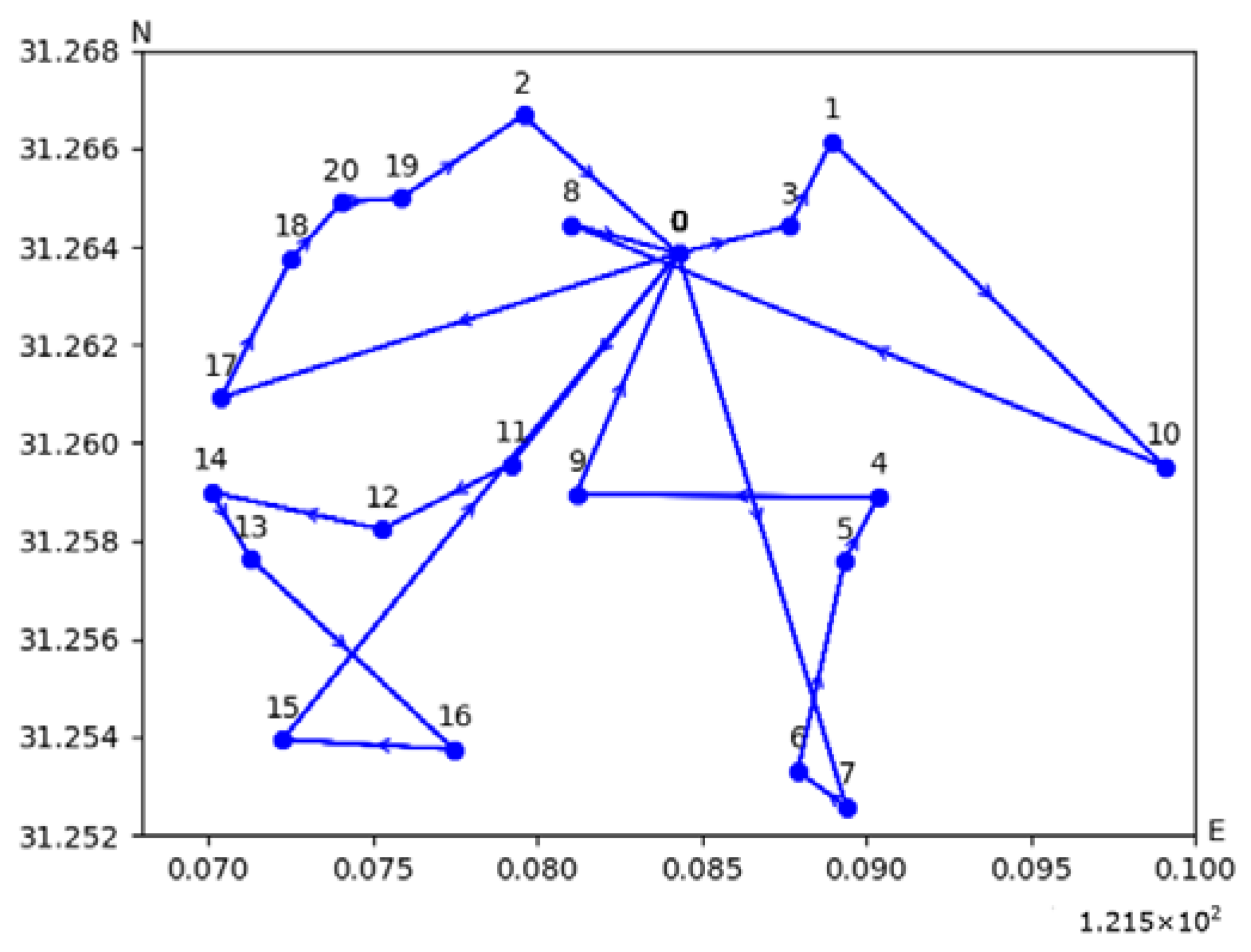
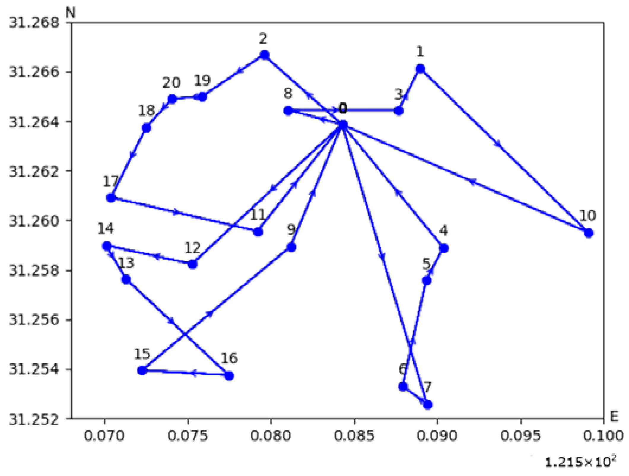
As indicated by Table 4, when considering a customer point scale of 10, 7 vehicles are required to complete a total of 7 trips under the single-trip strategy. However, in the multi-trip strategy, only one vehicle is needed to complete 6 trips. The multi-trip strategy results in fewer vehicle trips and lower fixed costs for vehicle activation, leading to reduced overall costs. The vehicle routes under the single-trip strategy are shown in Figure 8a, while the multi-trip vehicle routes are depicted in Figure 8b. A comparison of Figure 8a,b reveals that the routes under both strategies are similar, with minor differences in specific routing schemes. However, the multi-trip strategy proves to be more efficient in terms of vehicle resource utilization.

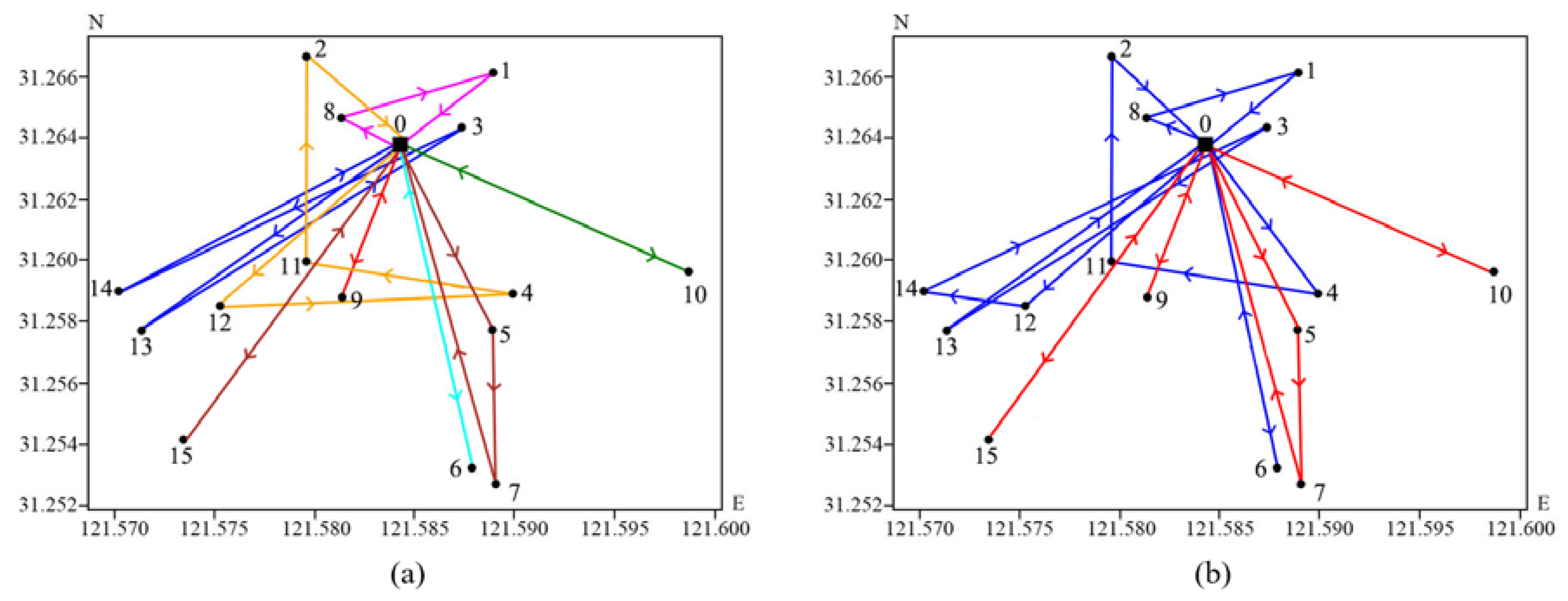
In the case with 15 customer points, the vehicle routing under the single-trip strategy is depicted in Figure 9a, while the multi-trip strategy’s vehicle routing is illustrated in Figure 9b. The routing schemes are broadly similar, but under the multi-trip strategy, only 2 vehicles are needed, making 4 trips, respectively, to complete the task. In contrast, the single-trip strategy requires 8 vehicles, each making a round trip to visit the customer points. Although the trip costs are the same, the reduced number of vehicles activated under the multi-trip strategy leads to lower fixed and total costs, higher equipment utilization rates, and a closer alignment with real operational conditions.

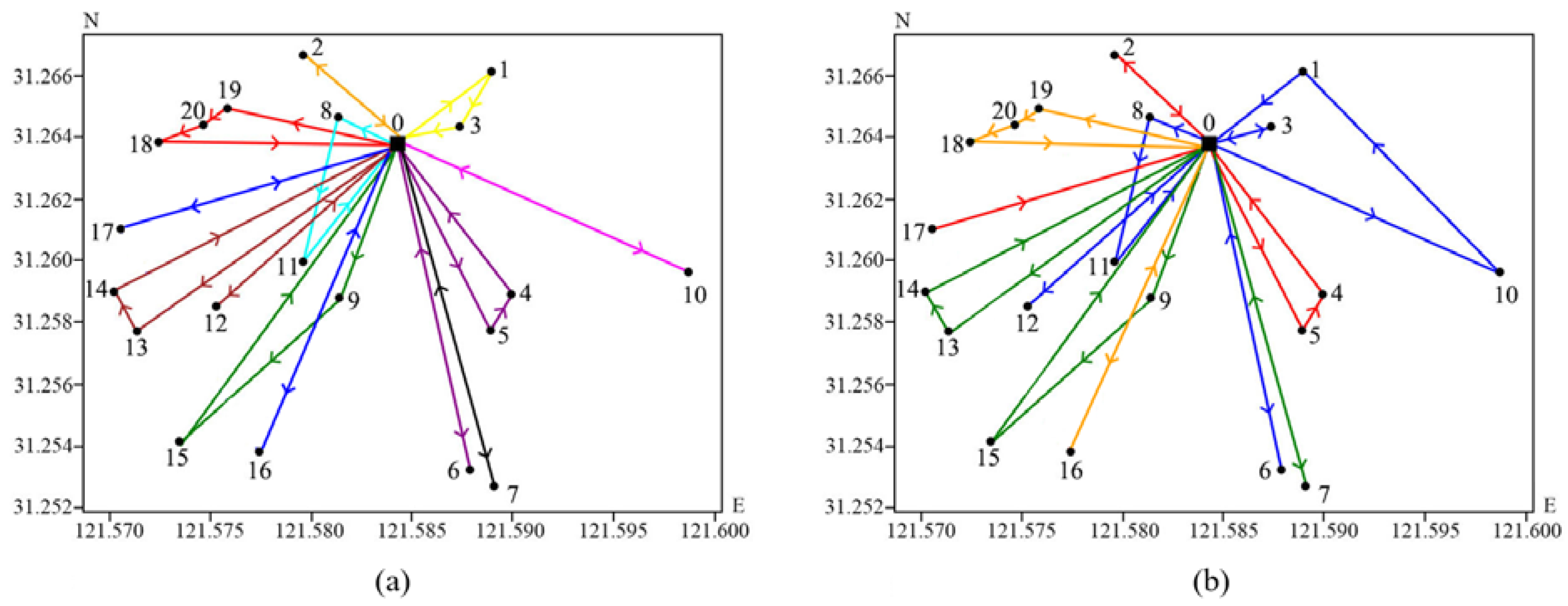
When facing 20 customer points, the routes for the single-trip strategy are presented in Figure 10a, while the multi-trip strategy’s vehicle route map is shown in Figure 10b. The single-trip strategy necessitates the use of 13 vehicles to complete 13 tasks each. In contrast, the multi-trip strategy requires only 4 vehicles to accomplish the same number of 13 trips. Consistent with the previous two case studies, the reduction in the number of vehicles used, while maintaining similar routes, leads to a decrease in the total vehicle operational costs.

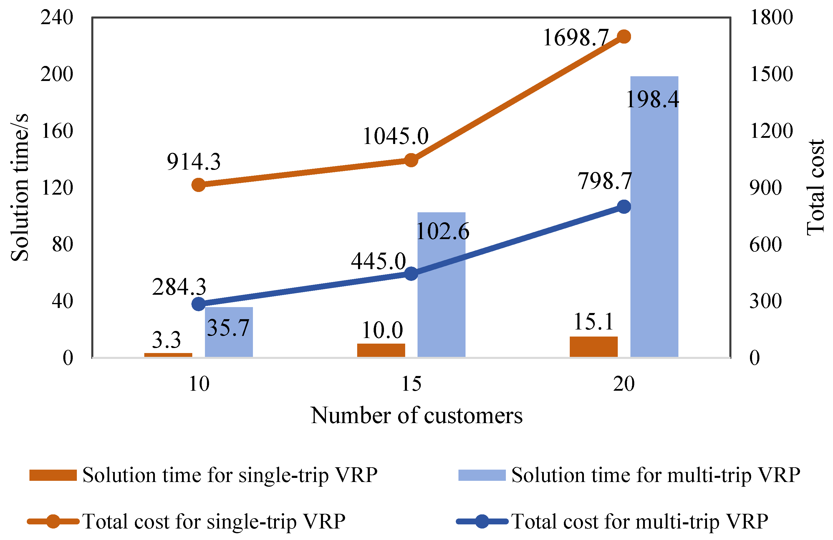
Furthermore, this paper also compares the solution time and total cost of the VRP under both strategies, as illustrated in Figure 11. As the number of customer points increases, the time required to compute the optimal solution extends. Under conditions of 10, 15, and 20 customer points, the VRP under the multi-trip strategy presents greater challenges and necessitates more time for resolution compared to the single-trip strategy. Additionally, in the multi-trip strategy, the increase in customer points may lead to a rise in the number of vehicle trips, resulting in an exponential growth in the decision variable’s solution space.

As the number of customer points increases, the total cost of vehicle distribution escalates for both single-trip and multi-trip strategies. From a cost perspective, due to the delivery range of small electric vehicles being between 3 and 5 km and the proximity of customer points, the overall transportation costs are relatively low. Consequently, the impact of different route selections on vehicle operating costs is minimal. However, it is evident that compared to the single-trip strategy, the multi-trip strategy significantly reduces the number of vehicles activated, decreasing the fixed cost of vehicle use and enhancing vehicle utilization, thereby reducing the overall logistics costs. With an increasing number of customers, the multi-trip strategy further diminishes the vehicle activation costs. Therefore, the application of the multi-trip strategy in the actual distribution of fresh e-commerce, particularly during periods of high order volume and at locations with numerous customer points, effectively lowers logistics costs.

5.4. Comparative Analysis of Upper Limit for Vehicle Capacity

Given that vehicle capacity limit is a critical parameter in multi-trip routing optimization, larger vehicle capacities allow for more cargo per trip. However, excessive loading might impede delivery efficiency, or surplus capacity could lead to high empty running rates and resource wastage. To explore the impact of vehicle capacity limits on routing schemes, this paper presents an analysis of the total cost implications at different vehicle capacity limits within the same time window, for customer point quantities of 10 and 20.

As shown in

Table 5. Comparison of capacity limit for vehicles with 10 and 20 customer points.

Instance	Capacity Limit (L)	Travel Cost	Activation Cost	Trip Cost	Total Cost	Number of Vehicles	Number of Trips	Vehicle Full Load Rate
10-1	10	3.86	100	150	253.86	1	5	92%
10-2	15	3.39	100	120	223.39	1	4	83%
10-3	20	3.02	100	90	193.02	1	3	97%
10-4	25	2.46	100	60	162.46	1	2	77%
10-5	30	2.32	100	60	162.32	1	2	63%
10-6	35	2.32	100	60	162.32	1	2	59%
20-1	10	8.69	300	330	638.69	3	11	84%
20-2	15	7.75	200	270	477.75	2	9	92%
20-3	20	5.62	200	180	385.62	2	6	96%
20-4	25	5.47	100	180	285.47	1	6	98%
20-5	30	4.62	100	120	224.62	1	4	94%
20-6	35	4.39	100	120	224.39	1	4	79%

, with 10 customer points, only one vehicle is activated, and the smaller the vehicle capacity limit, the greater the number of trips. When the vehicle capacity limit ranges from 25 L to 35 L, the number of trips does not decrease as the vehicle capacity increases, and the total cost changes minimally. Conversely, as the capacity increases, the full load factor drops from 97% to 59%, indicating that equipping the delivery vehicle with a 20 L refrigerated delivery box is more reasonable when servicing 10 customer points. When the number of customer points is 20, three vehicles are required at a capacity of 10 L, whereas expanding the vehicle capacity to 25 L reduces the number of vehicles needed to just one. However, once the capacity expands to 30 L, the number of trips stabilizes at four, with the total cost no longer decreasing as capacity increases. Expanding the vehicle capacity further actually increases the empty running rate, leading to resource wastage.

Based on the findings above, this paper selects the computational results for 20 customer points to analyze the total distribution cost and vehicle routing schemes. The routes for different vehicle capacity limits with 20 customer points are shown in Figure 12, Figure 13, Figure 14, Figure 15, Figure 16 and Figure 17.

Comparing Figure 12 and Figure 13, it can be seen that the 10 L capacity requires 3 vehicles, while the 15 L capacity requires only 2 vehicles, resulting in a reduction in vehicle activation cost and a significant reduction in the total cost. Comparing Figure 14 and Figure 15, at a vehicle capacity of 20 L, the number of vehicles is higher. When the capacity limit increases to 25 L, only one vehicle is activated, indicating higher delivery efficiency than at the smaller capacities of 10 L and 15 L. The comparison between the routing schemes at 20 L and 25 L capacities shows significant differences in both the order and the number of customer points visited per trip, resulting in a substantial variance in total costs.

When the vehicle capacity limit is increased to 30 L and 35 L, the total cost varies by less than 1%, with the number of vehicles used and the number of trips remaining constant. The computed routing schemes vary with the capacity limit, yet most customer points share similar delivery routes. For example, as shown in Figure 16 and Figure 17, the routes between customer points 6 and 7, as well as between 15 and 16, remain largely unaffected, indicating that the delivery sequence for customer points further from the front warehouse is minimally impacted. The primary variations in routes occur with customer points closer to the front warehouse.

In summary, as the vehicle capacity limit gradually increases, each trip can carry more cargo, leading to a reduction in both the number of vehicles activated and the number of trips made. Consequently, the total driving distance decreases, resulting in lower transportation costs, vehicle activation costs, and trip activation costs, thus reducing the overall cost. A vehicle capacity between 20 and 30 L can meet the delivery demands of 10–20 customer points within the time window, enhancing delivery efficiency and equipment utilization while minimizing the waste of space resources. However, exceeding the optimal vehicle capacity can result in a high empty running rate and decreased efficiency. Additionally, due to time window constraints, vehicles overloaded with cargo may not meet customer demands within the specified service time, potentially diminishing customer satisfaction.

6. Conclusions

This study examines the VRP in the two-echelon e-commerce logistics under the front warehouse mode, analyzing the transition between the two echelons and the characteristics of last-mile delivery in the second echelon. The issue is formulated as a 2E-MTCVRPTW, aiming to find the cost-optimal routing scheme for vehicles across both echelons. An MILP model was developed in this paper, integrating the characteristics of the MTVRP and 2E-VRP, and an improved GA was employed for solution derivation. Matrix encoding was used to codify two critical decisions: vehicle selection and route allocation. This was combined with neighborhood search to replace the mutation operations in the classical GA, enhancing the global and local search capabilities of the algorithm. The effectiveness of the model and the efficiency of the algorithm were validated through experiments with small-, medium-, and large-scale cases, as well as sensitivity analysis, yielding the following conclusions:

(1)

The improved GA exhibited superior optimization capabilities and solution efficiency for medium- and large-scale problems compared to CPLEX.

(2)

A comparative analysis of the multi-trip strategy demonstrated that it enhances vehicle utilization and reduces overall logistics costs compared to the single-trip strategy.

(3)

An analysis of the impact of different vehicle capacity limits on delivery costs and vehicle routing plans suggested that providing vehicles with appropriate capacity loading for servicing varying numbers of customers can increase vehicle utilization and reduce total operational costs.

Further research could be undertaken in the following areas: First, considering the uncertainty of consumer demand, along with the inventory status and replenishment strategies of front warehouses, studying the joint optimization of inventory routing could enhance the efficiency and stability of the front warehouse logistics network system. Moreover, urban traffic conditions are complex, and traffic peak hours often coincide with high-demand periods for front warehouse delivery services, leading to reduced vehicle speeds or even congestion. Therefore, incorporating time-varying factors such as traffic congestion would provide a closer approximation to real-world conditions.

References

- 2022–2027 China Fresh E-Commerce Industry Demand Forecast and Development Trend Outlook Report. Available online: https://www.askci.com/reports/20220914/0838456156925099.shtml (accessed on 13 May 2024).
- Cai, X.; Chen, J.; Xiao, Y.; Xu, X. Optimization and coordination of fresh product supply chains with freshness-keeping effort. Prod. Oper. Manag. 2010, 19, 261–278. [Google Scholar] [CrossRef]
- Ge, H.; Goetz, S.; Canning, P.; Perez, A. Optimal locations of fresh produce aggregation facilities in the United States with scale economies. Int. J. Prod. Econ. 2018, 197, 143–157. [Google Scholar] [CrossRef]
- Feng, Y.; Liu, Y.K.; Chen, Y. Distributionally robust location–allocation models of distribution centers for fresh products with uncertain demands. Expert Syst. Appl. 2022, 209, 118180. [Google Scholar] [CrossRef]
- Bozorgi, A.; Pazour, J.; Nazzal, D. A new inventory model for cold items that considers costs and emissions. Int. J. Prod. Econ. 2014, 155, 114–125. [Google Scholar] [CrossRef]
- Silbermayr, L.; Waitz, M. Omni-channel inventory management of perishable products under transshipment and substitution. Int. J. Prod. Econ. 2024, 267, 109089. [Google Scholar] [CrossRef]
- Dai, Z.; Aqlan, F.; Zheng, X.; Gao, K. A location-inventory supply chain network model using two heuristic algorithms for perishable products with fuzzy constraints. Comput. Ind. Eng. 2018, 119, 338–352. [Google Scholar] [CrossRef]
- Partovi, F.; Seifbarghy, M.; Esmaeili, M. Revised solution technique for a bi-level location-inventory-routing problem under uncertainty of demand and perishability of products. Appl. Soft Comput. 2023, 133, 109899. [Google Scholar] [CrossRef]
- Chen, H.K.; Hsueh, C.F.; Chang, M.S. Production scheduling and vehicle routing with time windows for perishable food products. Comput. Oper. Res. 2009, 36, 2311–2319. [Google Scholar] [CrossRef]
- Hu, H.; Zhang, Y.; Zhen, L. A two-stage decomposition method on fresh product distribution problem. Int. J. Prod. Res. 2017, 55, 4729–4752. [Google Scholar] [CrossRef]
- Soysal, M.; Bloemhof-Ruwaard, J.M.; Haijema, R.; van der Vorst, J.G. Modeling a green inventory routing problem for perishable products with horizontal collaboration. Comput. Oper. Res. 2018, 89, 168–182. [Google Scholar] [CrossRef]
- Song, B.D.; Ko, Y.D. A vehicle routing problem of both refrigerated-and general-type vehicles for perishable food products delivery. J. Food Eng. 2016, 169, 61–71. [Google Scholar] [CrossRef]
- Wu, F.; Dong, M. Eco-routing problem for the delivery of perishable products. Comput. Oper. Res. 2023, 154, 106198. [Google Scholar] [CrossRef]
- Ahmadi-Javid, A.; Mansourfar, M.; Lee, C.G.; Liu, L. Optimal distribution of perishable foods with storage temperature control and quality requirements: An integrated vehicle routing problem. Comput. Ind. Eng. 2023, 182, 109215. [Google Scholar] [CrossRef]
- Dantzig, G.B.; Ramser, J.H. The truck dispatching problem. Manag. Sci. 1959, 6, 80–91. [Google Scholar] [CrossRef]
- Laporte, G. Fifty years of vehicle routing. Transp. Sci. 2009, 43, 408–416. [Google Scholar] [CrossRef]
- Kafle, N.; Zou, B.; Lin, J. Design and modeling of a crowdsource-enabled system for urban parcel relay and delivery. Transp. Res. Part B Methodol. 2017, 99, 62–82. [Google Scholar] [CrossRef]
- Xia, Y.; Zeng, W.; Zhang, C.; Yang, H. A branch-and-price-and-cut algorithm for the vehicle routing problem with load-dependent drones. Transp. Res. Part B Methodol. 2023, 171, 80–110. [Google Scholar] [CrossRef]
- Tiwari, K.V.; Sharma, S.K. An optimization model for vehicle routing problem in last-mile delivery. Expert Syst. Appl. 2023, 222, 119789. [Google Scholar] [CrossRef]
- Chen, J.; Liao, W.; Yu, C. Route optimization for cold chain logistics of front warehouses based on traffic congestion and carbon emission. Comput. Ind. Eng. 2021, 161, 107663. [Google Scholar] [CrossRef]
- Chen, Q.; Liu, Z.; Tian, L.; Qin, X. In-store, pre-warehouse, or store-and-warehouse integration: Strategic analysis for neighborhood fresh product retail modes. Comput. Ind. Eng. 2023, 177, 109085. [Google Scholar] [CrossRef]
- Chen, W.; Zhang, Y.; Zhou, Y. Integrated scheduling of zone picking and vehicle routing problem with time windows in the front warehouse mode. Comput. Ind. Eng. 2022, 163, 107823. [Google Scholar] [CrossRef]
- Tang, J.; Qi, C.; Wang, H. Integrated optimization of order splitting and distribution routing for the front warehouse mode e-retailing. Int. J. Prod. Res. 2024, 62, 1715–1736. [Google Scholar] [CrossRef]
- Crainic, T.G.; Ricciardi, N.; Storchi, G. Models for evaluating and planning city logistics systems. Transp. Sci. 2009, 43, 432–454. [Google Scholar] [CrossRef]
- Perboli, G.; Tadei, R.; Vigo, D. The two-echelon capacitated vehicle routing problem: Models and math-based heuristics. Transp. Sci. 2011, 45, 364–380. [Google Scholar] [CrossRef]
- Soysal, M.; Bloemhof-Ruwaard, J.M.; Bektaş, T. The time-dependent two-echelon capacitated vehicle routing problem with environmental considerations. Int. J. Prod. Econ. 2015, 164, 366–378. [Google Scholar] [CrossRef]
- Wang, K.; Shao, Y.; Zhou, W. Matheuristic for a two-echelon capacitated vehicle routing problem with environmental considerations in city logistics service. Transp. Res. Part D Transp. Environ. 2017, 57, 262–276. [Google Scholar] [CrossRef]
- Li, H.; Liu, Y.; Jian, X.; Lu, Y. The two-echelon distribution system considering the real-time transshipment capacity varying. Transp. Res. Part B Methodol. 2018, 110, 239–260. [Google Scholar] [CrossRef]
- Dellaert, N.; Van Woensel, T.; Crainic, T.G.; Saridarq, F.D. A multi-commodity two-Echelon capacitated vehicle routing problem with time windows: Model formulations and solution approach. Comput. Oper. Res. 2021, 127, 105154. [Google Scholar] [CrossRef]
- Gu, W.; Archetti, C.; Cattaruzza, D.; Ogier, M.; Semet, F.; Speranza, M.G. A sequential approach for a multi-commodity two-echelon distribution problem. Comput. Ind. Eng. 2022, 163, 107793. [Google Scholar] [CrossRef]
- Sluijk, N.; Florio, A.M.; Kinable, J.; Dellaert, N.; Van Woensel, T. A chance-constrained two-echelon vehicle routing problem with stochastic demands. Transp. Sci. 2023, 57, 252–272. [Google Scholar] [CrossRef]
- Belgin, O.; Karaoglan, I.; Altiparmak, F. Two-echelon vehicle routing problem with simultaneous pickup and delivery: Mathematical model and heuristic approach. Comput. Ind. Eng. 2018, 115, 1–16. [Google Scholar] [CrossRef]
- Yan, X.; Huang, H.; Hao, Z.; Wang, J. A graph-based fuzzy evolutionary algorithm for solving two-echelon vehicle routing problems. IEEE Trans. Evol. Comput. 2019, 24, 129–141. [Google Scholar] [CrossRef]
- Anderluh, A.; Nolz, P.C.; Hemmelmayr, V.C.; Crainic, T.G. Multi-objective optimization of a two-echelon vehicle routing problem with vehicle synchronization and ‘grey zone’customers arising in urban logistics. Eur. J. Oper. Res. 2021, 289, 940–958. [Google Scholar] [CrossRef]
- Enthoven, D.L.; Jargalsaikhan, B.; Roodbergen, K.J.; Uit het Broek, M.A.; Schrotenboer, A.H. The two-echelon vehicle routing problem with covering options: City logistics with cargo bikes and parcel lockers. Comput. Oper. Res. 2020, 118, 104919. [Google Scholar] [CrossRef]
- Vincent, F.Y.; Jodiawan, P.; Hou, M.L.; Gunawan, A. Design of a two-echelon freight distribution system in last-mile logistics considering covering locations and occasional drivers. Transp. Res. Part E Logist. Transp. Rev. 2021, 154, 102461. [Google Scholar]
- Zhou, S.; Zhang, D.; Ji, B.; Li, S. Two-echelon vehicle routing problem with direct deliveries and access time windows. Expert Syst. Appl. 2024, 244, 121150. [Google Scholar] [CrossRef]
- Nguyen, P.K.; Crainic, T.G.; Toulouse, M. A tabu search for time-dependent multi-zone multi-trip vehicle routing problem with time windows. Eur. J. Oper. Res. 2013, 231, 43–56. [Google Scholar] [CrossRef]
- Masmoudi, M.A.; Hosny, M.; Braekers, K.; Dammak, A. Three effective metaheuristics to solve the multi-depot multi-trip heterogeneous dial-a-ride problem. Transp. Res. Part E Logist. Transp. Rev. 2016, 96, 60–80. [Google Scholar] [CrossRef]
- Hernandez, F.; Feillet, D.; Giroudeau, R.; Naud, O. Branch-and-price algorithms for the solution of the multi-trip vehicle routing problem with time windows. Eur. J. Oper. Res. 2016, 249, 551–559. [Google Scholar] [CrossRef]
- Neira, D.A.; Aguayo, M.M.; De la Fuente, R.; Klapp, M.A. New compact integer programming formulations for the multi-trip vehicle routing problem with time windows. Comput. Ind. Eng. 2020, 144, 106399. [Google Scholar] [CrossRef]
- Paradiso, R.; Roberti, R.; Laganá, D.; Dullaert, W. An exact solution framework for multitrip vehicle-routing problems with time windows. Oper. Res. 2020, 68, 180–198. [Google Scholar] [CrossRef]
- Roohnavazfar, M.; Pasandideh, S.H.R. Decomposition algorithm for the multi-trip single vehicle routing problem with AND-type precedence constraints. Oper. Res. 2022, 22, 4253–4285. [Google Scholar] [CrossRef]
- François, V.; Arda, Y.; Crama, Y.; Laporte, G. Large neighborhood search for multi-trip vehicle routing. Eur. J. Oper. Res. 2016, 255, 422–441. [Google Scholar] [CrossRef]
- Coelho, V.N.; Grasas, A.; Ramalhinho, H.; Coelho, I.M.; Souza, M.J.; Cruz, R.C. An ILS-based algorithm to solve a large-scale real heterogeneous fleet VRP with multi-trips and docking constraints. Eur. J. Oper. Res. 2016, 250, 367–376. [Google Scholar] [CrossRef]
- Zhen, L.; Ma, C.; Wang, K.; Xiao, L.; Zhang, W. Multi-depot multi-trip vehicle routing problem with time windows and release dates. Transp. Res. Part E Logist. Transp. Rev. 2020, 135, 101866. [Google Scholar] [CrossRef]
- Pan, B.; Zhang, Z.; Lim, A. Multi-trip time-dependent vehicle routing problem with time windows. Eur. J. Oper. Res. 2021, 291, 218–231. [Google Scholar] [CrossRef]
- Yağmur, E.; Kesen, S.E. Multi-trip heterogeneous vehicle routing problem coordinated with production scheduling: Memetic algorithm and simulated annealing approaches. Comput. Ind. Eng. 2021, 161, 107649. [Google Scholar] [CrossRef]
- Şahin, M.K.; Yaman, H. A branch and price algorithm for the heterogeneous fleet multi-depot multi-trip vehicle routing problem with time windows. Transp. Sci. 2022, 56, 1636–1657. [Google Scholar] [CrossRef]
- Marques, G.; Sadykov, R.; Dupas, R.; Deschamps, J.C. A branch-cut-and-price approach for the single-trip and multi-trip two-echelon vehicle routing problem with time windows. Transp. Sci. 2022, 56, 1598–1617. [Google Scholar] [CrossRef]
- Li, Y.; Yang, J. The last-mile delivery vehicle routing problem with handling cost in the front warehouse mode. Comput. Ind. Eng. 2024, 190, 110076. [Google Scholar] [CrossRef]
Figure 1.
The types of transport vehicles at different echelons of the front warehouse.
Figure 2.
The two-echelon supply chain network structure under front warehouse mode.
Figure 3.
Vehicle routing problem: (a) represents the Single-trip VRP and (b) represents the Multi-trip VRP.