Article

Systemic Modeling and Prediction of Port Container Throughput Using Hybrid Link Analysis in Complex Networks

School of Management, Shanghai University, Shanghai 200444, China
*
Author to whom correspondence should be addressed.
Systems 2024, 12(1), 23; https://doi.org/10.3390/systems12010023
Submission received: 3 December 2023 / Revised: 28 December 2023 / Accepted: 8 January 2024 / Published: 10 January 2024

Abstract

:
This paper introduces a hybrid framework for port container throughput forecasting, which is essential in global trade and transportation systems. It uses a multidisciplinary method that combines artificial intelligence, link prediction, and complex networks. To better grasp the interconnection and dynamics of port operations, time series data are first transformed using complex network theory into a network structure. The framework applies 13 similarity metrics, encompassing various aspects of network structural similarity, to form a feature set representing the complex port operation network. The most effective features are selected using the maximum relevance minimum redundancy (mRMR) method, adhering to systems theory’s efficiency principles. These features are processed through SVM, DNN, and LSTM models for link prediction, which is crucial for forecasting in port logistics. Finally, the methodology concludes with regression analysis to obtain container throughput forecasts, which is a key metric in port systems management. Case studies of Shanghai Port and Shenzhen Port validate the framework’s effectiveness, demonstrating a significant improvement in forecasting accuracy over the baseline models. This study contributes to systems analysis by showcasing a hybrid, AI-enhanced approach for managing and forecasting critical aspects of maritime trade systems.

1. Introduction

Within the framework of systems theory, trade integration and economic globalization are heavily dependent on the systemic operation of port logistics, which constitutes the bedrock of the global economy. Ports, as critical nodes in international trade, play a vital role in the global logistics network, underscoring the interdependent nature of the global economic system. Container shipping, as the predominant mode of international freight transport, is characterized by its high efficiency and low cost, emerging as the dominant form of maritime transportation [1], and symbolizing the close-knit connections of the global economy. From the perspective of systems analysis, port planning extends beyond mere physical infrastructure; it encompasses resource allocation, transportation management, and local economic development, each of which is an integral component of the global economic system. The accurate forecasting of port container throughput is of paramount importance, serving not only as a key metric for assessing system efficiency but also providing a crucial basis for strategic decision-making in resource allocation and transportation management. With the increasing interconnectedness of the world economy, such forecasts are indispensable for enhancing the responsiveness of the system and supporting sustained growth.
This article focuses on proposing a hybrid forecasting model that integrates complex networks, link prediction, and artificial intelligence algorithms to enhance the predictive performance of container throughput. The rest of the work is structured as follows. Section 2 reviews past studies related to the forecasting of container throughput. Section 3 discusses the research methods used in the proposed forecasting framework of this paper. Section 4 presents the forecasting results. Finally, Section 5 summarizes the research findings of this paper, identifies its limitations, and provides an outlook for future research.

2. Literature Review

Since the 1980s, scholars have extensively researched the forecasting of port container throughput, mainly employing three types of forecasting methods: econometric models, artificial intelligence models, and combined forecasting approaches. Econometric models use statistical models to forecast port container throughput, with the Autoregressive Integrated Moving Average (ARIMA) [2] model being the most widely applied. However, these models primarily capture the linear characteristics of the data. As processing power and artificial intelligence technologies grow, machine learning and deep learning models, which are adept at depicting the nonlinear features of data, have been widely used in forecasting domains such as exchange rate forecasting [3] and electric load forecasting [4]. Notably, Fan et al. [5] used the NARX neural network model to forecast container throughput at Shanghai Port, demonstrating its effectiveness in capturing complex nonlinear relationships in data for accurate predictions. Port container throughput, influenced by the hinterland economy, policy environment, and seasonality, exhibits considerable uncertainty in the original series, making it challenging for a single model to adequately represent the data. Consequently, scholars have proposed hybrid forecasting models that combine various individual methods. For instance, Huang et al. [6] applied local outlier factors for anomaly detection in time series and designed a hybrid model based on projection pursuit regression and genetic programming (GP) for predicting container throughput at Qingdao Port. The findings showed that hybrid forecasting models have higher prediction accuracy and robustness compared to single models.
Time series analysis and forecasting have been gradually incorporated into complex network theory, which has been widely applied in recent years in fields like bioinformatics, social networking, and financial risk control. Analyzing time series data patterns and structural features forms the basis of this approach. Lacasa is credited with the significant creation of the visibility graph technique, which maintains low computing complexity while changing time series into networks with nodes and edges [7]. It does this by preserving the fluctuation properties of the data. Time series forecasting is made easier by examining the altered network’s topological structure. Building on this algorithm, subsequent studies, like the limited penetrable visibility graph, which was proposed by Zhou [8], further improved the ability to handle noise. Additionally, Ma [9] and other scholars proposed the multivariate visibility graph for handling multivariate time series. Despite these improvements, the visibility graph algorithm remains advantageous in practical applications due to its simplicity and low complexity.
One important mission in the study of complex networks is link prediction, which depends on the analysis of node information and network architecture to forecast the possibility of links between nodes. The information included in the network’s topological structure is the central focus of classic link prediction algorithms, which estimate node similarity using three different kinds of similarity measures in line with local, semi-local, and global information. Among them, techniques depending on individual node characteristics, like the Jaccard and Common Neighbors (CN) similarity indices, focus on the direct connections between nodes and, because of their high computing efficiency, are appropriate for vast networks. Methodologies combined with semi-local node information have limited applicability across different network types, while those based on global node information consider the entire network’s structure but are not suitable for big networks owing to their higher computational power. Given the significant structural differences between networks, these methods may perform well in some networks but not in others. In recent years, scholars in link prediction research have tended to integrate multiple similarity indices to obtain a composite similarity value and make link predictions based on this value to achieve better prediction results. Therefore, the selection of similarity indices and the determination of integration weights are particularly crucial. Liu et al. [10] used the Ordered Weighted Averaging (OWA) algorithm to obtain weights for various similarity indices. A linear framework was presented by Zhang et al. [11] to integrate different single similarity indices, but this method only used connected node pairs to establish the linear regression model, ignoring the impact of indirectly connected node pairs. Thus, in link prediction research, how to select similarity indices is an urgent problem to be solved, as it greatly influences the prediction results. In the last few years, many scholars have considered the value of the paths between two nodes in link prediction research. Ayoub et al. [12] discussed the impact of using paths of different lengths as a parameter in the accuracy of indices. Their research showed that good prediction accuracy could be achieved when the path length is two or three. Meanwhile, with the popularity of artificial intelligence algorithms, scholars have begun to explore combining machine learning algorithms for link prediction research. In these studies, in addition to network representation learning and graph neural networks, machine learning binary classification models based on network topology characteristics and local node feature information also have good applicability. Güneş et al. [13] combined the topological structure similarity indices of static networks with the ARIMA model, and the proposed time-series link prediction algorithm achieved good experimental results.
Based on the aforementioned analysis, the main research gaps in the field of port container throughput include an insufficient application of complex network theory in the prediction of port container throughput, particularly in aspects of link prediction and the transformation of time series data into network structures. Furthermore, existing research predominantly focuses on traditional predictive models, with inadequate exploration of hybrid forecasting frameworks that integrate complex network theory and artificial intelligence algorithms. Additionally, current research on the applicability and effectiveness of different network structural features and link prediction algorithms in the prediction of port container throughput remains relatively limited. In light of these observations, this study employs a combination of complex network theory, link prediction, and artificial intelligence models to analyze and forecast port container throughput, considering the analysis that was previously presented. The main contributions of this study are as follows: (1) By utilizing the visibility graph algorithm, time series data can be transformed into a network structure. This transformed network incorporates the feature information of links between nodes, which enables automatic learning of these features for link prediction. As a result, the forecasting results become more stable due to the enhanced ability to predict links between connected nodes. This approach is particularly effective in revealing dynamic relationships and patterns within port transportation networks, offering a unique perspective compared to traditional data-driven forecasting methods; (2) By adding second-order path information, the modified network’s structural properties are more accurately represented, node interactions and associations are captured and analyzed with better accuracy, and the structural information for prediction is more richly represented; (3) The paper introduces 13 single-mechanism index signals of network structure similarity from local, semi-local, and global viewpoints and offers the idea of integration. Better forecasting results are obtained by choosing feature indicators that are appropriate for the network structure of this article using the maximum relevance minimum redundancy algorithm (mRMR).

3. Methods

3.1. Theory of Complex Networks

3.1.1. Complex Networks and Their Topological Properties

Complex networks serve as a vital tool in the study of time series data, typically represented using nodes and connecting edges. The theoretical foundation of complex networks lies in graph theory, where a network is defined as G = V , E , with V = v 1 , v 2 , , v N representing the group of nodes, and E denoting the set of edges or links [14]. Networks can be classified as directed unweighted networks, undirected weighted networks, directed weighted networks, or undirected unweighted networks based on the type of connections that exist between nodes. The network G is a simple, undirected, unweighted network with N nodes and M edges. The adjacency matrix A = ( a i j ) N × N of network G is an N -order real symmetric matrix. If there exists an edge ( v i , v j ) E , then the elements within the ith row and jth column of A are denoted as a i j = 1 ; otherwise, they are set to 0.
The primary topological characteristics of networks include degree and average degree, average path length, and clustering coefficient. They are detailed as follows:
(1)
The Degree
One of the most basic and straightforward ideas for describing the characteristics of individual nodes is the degree. In an undirected network, the degree k i of node i is defined as the number of edges directly connected to node i . For simple graphs without self-loops and multiple edges, the degree k i of node i also represents the number of other nodes directly connected to the node i .
(2)
Average Degree
The term “network average degree” refers to the average degree value for all nodes inside the network., denoted as ‹ k ›. Given the adjacency matrix A = ( a i j ) N × N of network G , we have:
k = 1 N i = 1 N k i = 1 N i , J = 1 N a i j = 1 N i , j = 1 N a j i
where k i represents the degree of the network and N is the number of nodes in the network.
(3)
Average Path Length
In the theory of complex networks, the distance between nodes defines the number of shortest path edges, and the mean length of the path l of the entire network refers to the average distance between all pairs of nodes. Its formula is as follows:
l = 1 N N 1 i , j V i j d i s i , j
where N represents the number of nodes in the network, V represents the set of nodes in the network, and d i s i , j represents the distance between node i and node j .
(4)
Clustering Coefficient
The clustering coefficient, which represents the density of the network and shows how many common neighbors connected nodes share, is used to characterize how network nodes cluster together. For node i , its clustering coefficient C i can be computed using the formula:
C i = 2 E i k i k i 1
where k i represents the degree of node i and E i denotes the actual number of edges among these k i nodes. The average of the clustering coefficients of all nodes is the clustering coefficient for the network as a whole, and its formula is as follows:
C = 1 N i C i

3.1.2. Visual Graph Algorithm

Time series data can be mapped into a network using the Visual Graph Algorithm [7], which visualizes the time series’ geometric characteristics. For a set of time series data, S = { t 1 , y 1 , t 2 , y 2 , , t i , y i , , t N , y N } , where y i denotes the value at the time point t i . In the visual graph, each point in the time series is considered a node. For any two nodes ( t a , y a ) and ( t b , y b ) in the time series, if there exists any data point ( t c , y c ) satisfying the principle of visibility inequality Equation (5), then ( t a , y a ) and ( t b , y b ) are considered visible.
y c < y b + y a y b t b t c t b t a
Three basic aspects characterize the visual graph created by the visual graph algorithm:
(1)
Connectivity: Every node is viewable to at least its closest neighbors, forming an interconnected network;
(2)
Undirectedness: Links are not directed;
(3)
Stability: If the horizontal and vertical coordinates of the time series are scaled, the principle of visibility remains unchanged.

3.2. Concepts of Link Prediction

3.2.1. Description of Link Prediction Problem

A basic topic in network science is link prediction, which involves forecasting when two disconnected nodes will form a link or deduce missing links in a network. Taking an undirected, unweighted simple network G as an example, if all nodes in the network are linked, there are a total of N ( N 1 ) / 2 edges and the set of unlinked links is denoted as U E . Link prediction involves providing the topological structure of the network G at time T and predicting the topological structure of the network G at time T + Δ t , as shown in Figure 1 (Circular numbers represent nodes, solid lines represent existing connections and the red dashed lines represent the predicted potential links).
To assess the accuracy of link prediction algorithms, the link prediction dataset (link set) is split into a training set E T and a test set E P . The network information in the training set E T is primarily used for training and learning, while the test set E P is employed to assess the link prediction accuracy of the algorithm. It is essential to ensure that E = E T E P and the intersection between E T and E P is empty.

3.2.2. Measurement of Network Structural Similarity

To forecast future connections, link prediction algorithms use the structural information of a network to calculate the similarity scores for two node pairs. Three types of structural information about a network exist, global, semi-local, and local, which correlate to different kinds of similarity measures.
Similarity methods based on local information utilize structural information related to node neighborhoods to determine how similar each node is to the other nodes in the network. These approaches have great parallelism and are faster than non-local approaches. Specifically:
(1)
C N Index: The similarity between two nodes is defined as the number of shared neighbors between the two nodes [15]. This index defines the similarity function as follows:
C N i , j = Γ i Γ j
where Γ i Γ j represents the set of common neighbors between node i and node j , and the symbol · denotes the number of elements in a set;
(2)
A A Index: This similarity measure aims to quantify the similarity between two entities based on their shared features [16]. If we consider neighbors as features, it can be expressed as:
A A i , j = z Γ i Γ j 1 log Γ z
where Γ i Γ j represents the set of common neighbors between node i and node j , | Γ z | is the number of common neighbors z , and the logarithmic function l o g is used to reduce the weight of nodes with a large number of neighbors;
(3)
R A Index: The idea behind such an index is to compare the challenge of creating connections inside a network to the process of allocating resources [17]. It simulates the transfer of resources between two disconnected nodes i and j through neighboring nodes. The similarity function is expressed as:
R A i , j = z Γ i Γ j 1 | Γ z |
where Γ i Γ j represents the set of common neighbors between node i and node j , and | Γ z | is the number of common neighbors z ;
(4)
P A Index: This index is based on the assumption that new connections in the network are more likely to occur between nodes that already have a higher number of connections. According to this assumption, a likelihood score is derived for the existence of a link between two nodes [18]. The similarity is defined as:
P A i , j = k i × k j
where k i and k j are the degrees of nodes i and j , respectively;
(5)
J a c c a r d Index: This frequently used coefficient is used to compare the variety and similarity of sample sets in information retrieval systems [19]. It calculates the proportion of unique neighbors in two nodes’ combined neighborhoods to the common neighbors between them. It is defined as:
J a c c a r d i , j = | Γ i Γ j | | Γ i Γ j |
where | Γ i Γ j | is the number of common neighbors between node i and node j , and | Γ i Γ j | is the total number of neighbors for both nodes;
(6)
H P I Index: This index was introduced to address modularity in metabolic networks, characterized by a hierarchical structure where interconnected modules are isolated from each other [20]. The primary objective of this similarity measure is to discourage link formation between hub nodes while encouraging link formation between low-degree nodes. The specific definition of the H P I index is not provided in the given context. It is defined as:
H P I i , j = min ( k i , k j )
These similarity algorithms, which are based on semi-local information, take into account more information than local indicators and ignore redundant data that adds little to no value to prediction accuracy. Specifically:
(1)
Local Random Walk ( L R W ) Index: L R W is a technique based on random walks, simulating a random walker starting from a source node and moving to neighboring nodes with a certain probability, continuing until a specific number of steps or conditions are met. The walker records the sequence of nodes traversed, typically considering only nodes reached within a certain number of steps. It is defined as:
L R W i , j = | Γ i | 2 E p j i t + | Γ j | 2 E p i j t
where | Γ x | and | Γ y | represent the number of common neighbors of nodes i and j , E is the total number of edges in the network, p j i t denotes the probability of visiting node i at step t , and p i j t is the probability of visiting node j at step t ;
(2)
Superimposed Random Walk ( S R W ) Index: This index considers the degree of overlap between random walk paths between two nodes [21]. This behavior can be captured by summing the contributions of each walker as follows:
S R W i , j = i = 1 t | Γ i | 2 E p j i i + | Γ j | 2 E p i j i
(3)
F L Index: Just like the Local Path Index, F L is a quasi-local metric based on path counts between nodes of interest [22]. This method incorporates normalization and additional path-length penalty mechanisms. The similarity between two nodes x and y is calculated as follows:
F L x , y = i = 2 l 1 i 1 ( A i ) x , y j = 2 i V j  
where i is the path length, l is the maximum path length, ( A i ) x , y represents the number of paths of length i from node x to node y , and V represents the total number of nodes in the graph.
Techniques for calculating similarity that rely on global information assess each link by using the network’s overall topology. Specifically, it is as follows:
(1)
K a t z Index: This measure penalizes longer paths according to their length by adding up the influence of all feasible paths between two nodes [23]. It is defined as:
K a t z i , j = l = 1 β l p a t h s i , j l
where p a t h s x , y l is the set of paths of length l between nodes i and j , and β l is the decay factor corresponding to these path lengths, satisfying 0 < β < 1;
(2)
The Average Commute Time ( A C T ) Index: This measure represents the average number of steps needed for a random walker to start at node i, go to node j, and then return to node i. It has the following definition:
A C T i , j = k = 1 , k 0 N 1 λ k ( ϕ k i ϕ k j ) 2
where N is the graph’s overall number of nodes, λ k is the k th non-zero eigenvalue of the Laplacian matrix, and ϕ k i and ϕ k j are components of the eigenvector corresponding to the k th eigenvalue for nodes i and j , respectively;
(3)
L H N I I Index: In addition to the number of shared neighbors, the degree of those neighbors also influences the probability of an edge living among both two nodes. The following is the computation formula:
L H N I I i , j = | N i N j | k i × k j
(4)
M F I Index: The main concept of this index is to construct a “matching forest”, which is a set of node pairs that exist in both graphs and exhibit similar connection patterns. The following is the calculating formula:
M F I i , j = I + L 1
where I stands for the identity matrix, and L represents the Laplacian matrix.

3.2.3. Link Prediction Considering Second-Order Path Information

In the network G = V , E , each edge represents a direct connection between two nodes, which is considered as first-order path information. If in the network, two nodes are not directly connected by a single edge but can reach each other through a third node (as an intermediary), then the path between these two nodes is defined as second-order path information. Let us assume a network G = V , E with a node set V = v 1 , v 2 , v 3 , v 4 and an edge set E = ( v 1 , v 2 ) , ( v 1 , v 3 ) , ( v 2 , v 4 ) , ( v 3 , v 4 ) , as shown in Figure 2.
Thus, the first-order path information for node v 1 consists of the edges connecting v 2 and v 3 , as well as the node information. Conversely, the second-order path information for node v 1 includes the information on nodes and edges contained in v 4 , in addition to what is in v 2 and v 3 . By combining the structural information of nodes and the structural information of node neighbors, the node similarity considering second-order paths is redefined as shown in Equation (19):
S x y * = S x y + α S x y 2
In this context, S x y represents the similarity matrix for first-order paths and S x y 2 represents the similarity matrix for second-order paths. The parameter α , which serves as a tuning parameter, reflects the influence of second-order neighbor nodes on the structural similarity of nodes and can be chosen based on the specific network. When α is set to 0, S x y * represents the similarity matrix for first-order paths. Second-order path information is used in this study to anticipate links. We have, therefore, established α ∈(0,1). This is because experimental results have demonstrated that α falls within the range of (0, 1), where forecasting performance reaches a peak [24]. Moreover, the impact of second-order neighbor information on node similarity is smaller than that of first-order neighbor information. We used a 0.1 step size to choose various α values for our controlled tests.

3.3. The Maximum Relevance Minimum Redundancy Algorithm

For feature selection, the Maximum Relevance Minimum Redundancy algorithm (mRMR) is commonly employed. Its goal is to extract a subset of characteristics with low duplication from a dataset that has a strong correlation with the final output. The main goal of this algorithm is to boost the effectiveness of data representation by reducing unnecessary features, thereby enhancing the performance of models. It employs mutual information-based maximum statistical dependency between features [25]. Let X and Y be two discrete variables. Then, the following is a definition of their mutual information:
I X ; Y = y Y x X p x , y ln p x , y p x p y
where p x and p y represent the marginal probabilities of x and y , and p x , y   is the joint probability.
Finding a feature subset S among the m features { X i } that collectively exhibits the maximum dependence on the target class c is the goal of feature selection. Maximum dependence is expressed as:
D = 1 S X i S I X i ; c
where X i represents the i -th feature, c is the class variable, and S is the feature subset.
In addition, to eliminate variables that are redundant due to their inherent correlation, we introduce minimum redundancy:
R = 1 S 2 X i , X j S I X i ; X j
where I X i ; X j represents the mutual information between feature i and feature j .
mRMR combines the two limitations mentioned above and achieves the following conditions by simultaneously optimizing D and R :
m a x   ϕ D , R , ϕ = D R
To prevent the issue of unstable results that may arise from using a single structural similarity measurement method for link prediction, this paper uses the mRMR algorithm to select the appropriate similarity measurement indicators for the network structure to conduct link prediction. This is due to the advantages and disadvantages of the three types of structural similarity measurement methods in networks with different structural features.

3.4. Artificial Intelligence Algorithms

Given that AI models excel in handling complex patterns within data, they contribute to the enhancement of the accuracy of predictions. In this paper, we selected Support Vector Machine (SVM), Deep Neural Networks (DNN), and Long Short-Term Memory (LSTM) models for identifying network features to predict links.

3.4.1. Support Vector Machine (SVM)

Support Vector Machine (SVM) [26] is a machine learning strategy centered around the concept of statistical learning. The fundamental idea behind SVM for predictive analysis is to map input samples to a space with several dimensions R n using a special mapping function φ x , where the samples in R n are linear. Therefore, predictive analysis can be accomplished by employing linear regression methods in R n , and its functional relationship is as follows:
f x = ω · φ x + b
where ω , b , and f x represent the weight coefficients, bias term, and the predicted value for sample x , respectively.
For the linear regression problem, to make the resulting function f x as smooth as possible, it is necessary to find a small weight, which transforms the linear regression problem into a constrained optimization problem. By using relaxation techniques with the introduction of two relaxation variables ξ i and ξ i * , an objective optimization problem can be formulated as a solution to the linear regression problem.
m i n 1 2 ω 2 + c i = 1 n ξ i + ξ i *
s . t . y i ω · x i b ε + ξ i ω · x i + b y i ε + ξ i * ξ i 0 ξ i * 0 , i = 1,2 , , n
where c is the penalty parameter that controls the extent of penalty for sampling error ε .
To further solve the above formula, incorporating all constraints into a multivariate function, using the Lagrange algorithm to transform the constrained objective optimization problem into a system of linear equations analytically, and ultimately obtaining the model’s prediction value:
f x = i = 1 n a i + a i * K x i , x j + b

3.4.2. Long Short-Term Memory (LSTM)

LSTM is a special type of Recurrent Neural Network (RNN) capable of handling sequential data with long-range dependencies among its elements [27]. Its main principle involves utilizing internal states to uncover dependencies between elements in the sequence. It comprises forget, input, and output gates to address the shortcomings encountered during RNN gradient updates. The internal structure of a single-layer LSTM is depicted in Figure 3.
(1)
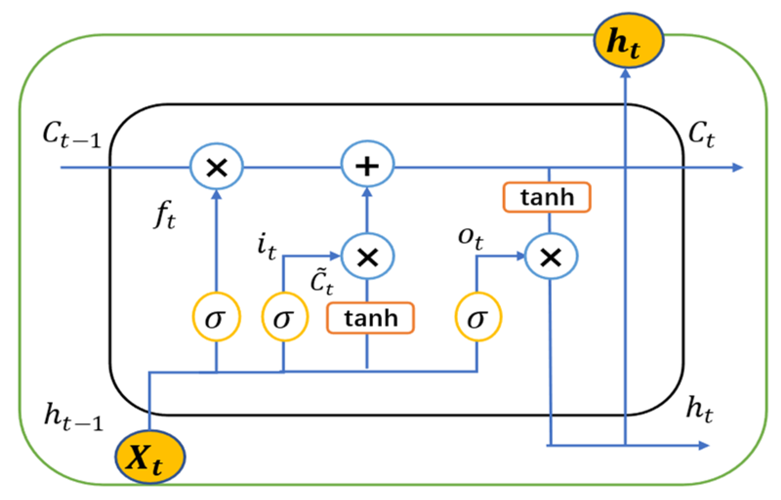
The forget gate is a key component of the LSTM model, and its primary role is to control the memory storage within the network to better handle long sequential information. The forget gate first linearly transforms the output from time t 1 with the input x t at time t . It then uses a sigmoid activation function to map the output to the [0, 1] interval, indicating the degree of forgetting the previous time step’s memory state. When the output of the forget gate is close to 1, the memory state from time t 1 is fully retained. When the forget gate’s output is nearly 0, the memory state from time t 1 is completely forgotten. The formula for the forget gate is:
f t = σ W f [ h t 1 , x t ] + b f
(2)
The input gate is used to determine which information from the input data will be passed to the subsequent time step at the previous time step. The input gate uses the same calculating technique as the forget gate. The formula for the input gate is:
i t = σ W i [ h t 1 , x t ] + b i
(3)
The state unit of LSTM is an important internal variable used to store information at time t and is updated through the control of the forget gate, input gate, and output gate. The formula for calculating the internal state at the current time step is:
C ~ t = i t × C t + f t × C t 1
C t = t a n h W C [ h t 1 , x t ] + b C
(4)
The output gate of the LSTM model is used to determine which information will be transmitted to the next time step. The output gate is made up of a multiplication of elements and a sigmoid activation function. The function of sigmoid responsible for determining the information to be output, while the element-wise multiplication regulates the importance of other information in the output state. Therefore, the output gate controls which information is passed to the output. The formula for the output gate is:
o t = σ W o x t + U o h t 1 + V o C t + b o
h t = o t × s i g m C t
where σ ( ) is the Sigmoid activation function, t a n h ( ) is the hyperbolic tangent function, W f , W i , and W C are the weight matrices for the respective layers, h t 1 , x t represents the concatenation of the previous time step’s output h t 1 and the current time step’s input x t , C ~ t is the internal state at time t , C t 1 is the internal state at time t 1 , f t is the forget gate, i t is the input gate, and C t is the input state at time t .

3.4.3. Deep Neural Network (DNN)

A Deep Neural Network (DNN), also known as a multi-layer perceptron, consists of three types of layers: input layer, hidden layers, and output layer. There are several neurons in each layer, and all neurons in each layer are fully connected, as shown in Figure 4.
In addition, the output value of a single layer in the DNN is represented by the following equation:
y ^ k = f 0 l = 1 r [ w l 0 f l h 2 ( j = 1 q w l j h 2 f j h 1 i = 1 p w j i h 1 x i k + b j h 1 + b l h 2 ) + b o ]
where x i k i = 1, 2, …, p ; k = 1, 2, …, n represents the variable used for input, and the output variable’s fitted value is denoted by y ^ k , where k is the pairing index value for the input and output variables ( x i k , y ^ k ). The weight w j i h 1 is for the i t h input leading to the j t h neuron in the first hidden layer ( j = 1, 2, …, q ), and b j h 1 is the bias in the j t h neuron of the first hidden layer. The function f j h 1 is the activation function at the j t h neuron in the first hidden layer, the weight w l 0 is for the l th neuron in the output layer coming from the second hidden layer, and b o is the bias at the neuron in the output layer. The function f 0 is the activation function at the neuron in the output layer. The weight w l j h 2 is for the l th neuron in the first hidden layer leading to the j t h neuron in the second hidden layer ( l = 1, 2, …, r ), b l h 2 is the bias at the l th neuron in the second hidden layer, and f l h 2 is the activation function at the l th neuron in the second hidden layer.

3.5. Overall Prediction Framework

In light of the noteworthy nonlinear and intricate features of port container throughput time series, this paper presents a predictive framework that integrates artificial intelligence models, complex networks, and link prediction for analysis and forecasting. It is based on the methods and principles discussed above. The application of these methods in the context of port container throughput is relatively novel, and they collectively contribute to a more accurate and robust forecasting framework. The four primary stages of the proposed predictive framework are feature selection, link prediction, output prediction value, and network creation of container throughput time series. Figure 5 is an illustration of the research framework.
In particular, this framework consists of the following four stages:
(1)
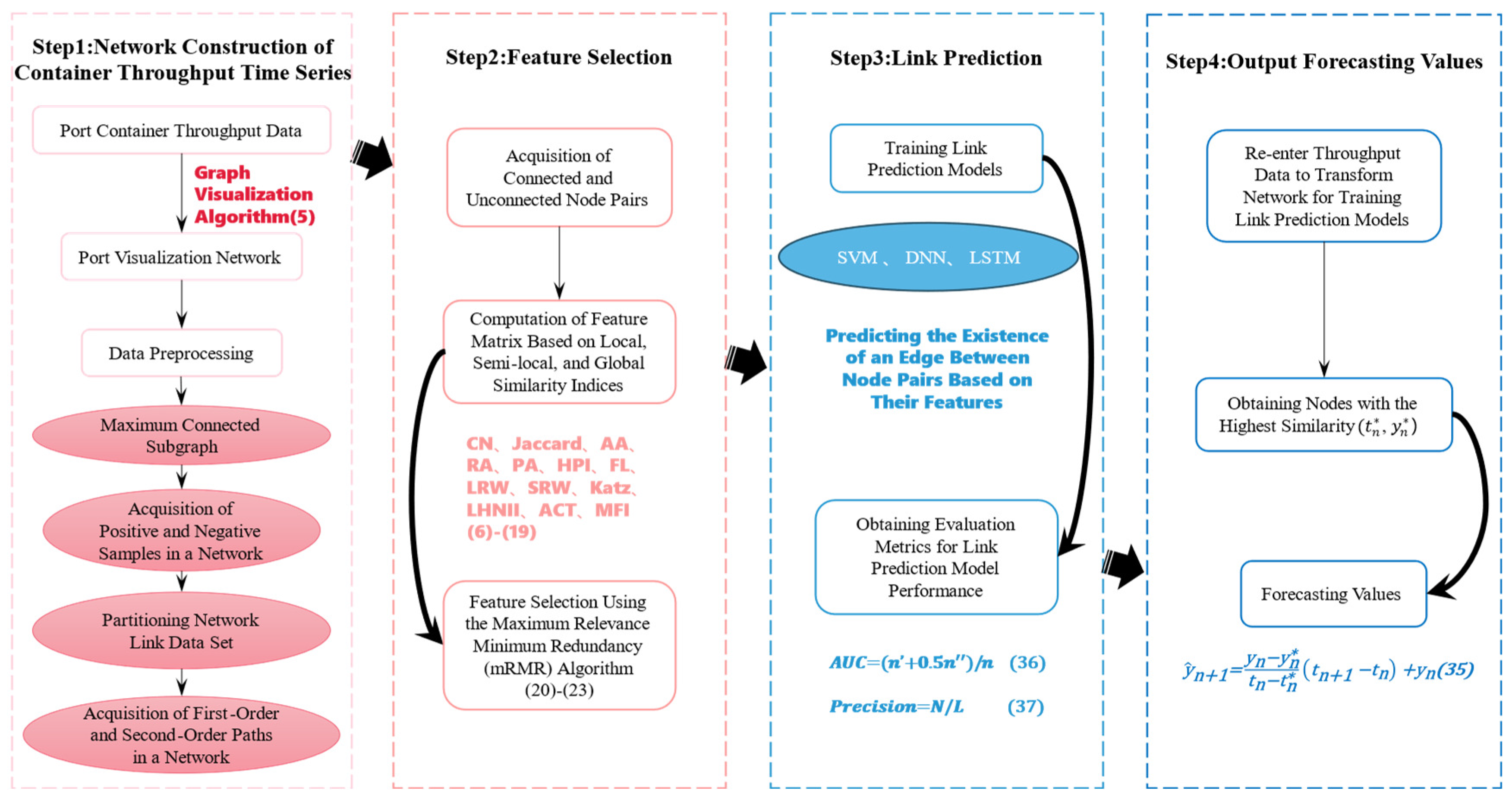
Network construction of container throughput time series: Initially, the port container throughput time series is transformed into a corresponding visual graph network using the visual graph algorithm (as shown in Equation (5)) in complex networks. The monthly dataset of port container throughput is examined to examine the network’s topological properties, including clustering coefficient and network diameter. Subsequently, the link dataset is partitioned based on the transformed visual graph network, and first-order and second-order path information of the corresponding network’s largest connected component is obtained;
(2)
Feature selection: Connected and unconnected node pairs are extracted from the obtained network. Thirteen similarity metrics, proposed from the perspectives of local, semi-local, and global network structural similarity (as shown in Equations (6)–(18)), are used as the feature set for complex networks. Feature selection is performed using the Maximum Relevance Minimum Redundancy method to extract properties of the structural network and capture latent information within the network (as shown in Equations (20)–(23));
(3)
Link Prediction: The selected features are used as inputs for training SVM, DNN, and LSTM models to perform link prediction. This means predicting whether there is an edge (1 for existence, 0 for non-existence) between each pair of nodes based on their features;
(4)
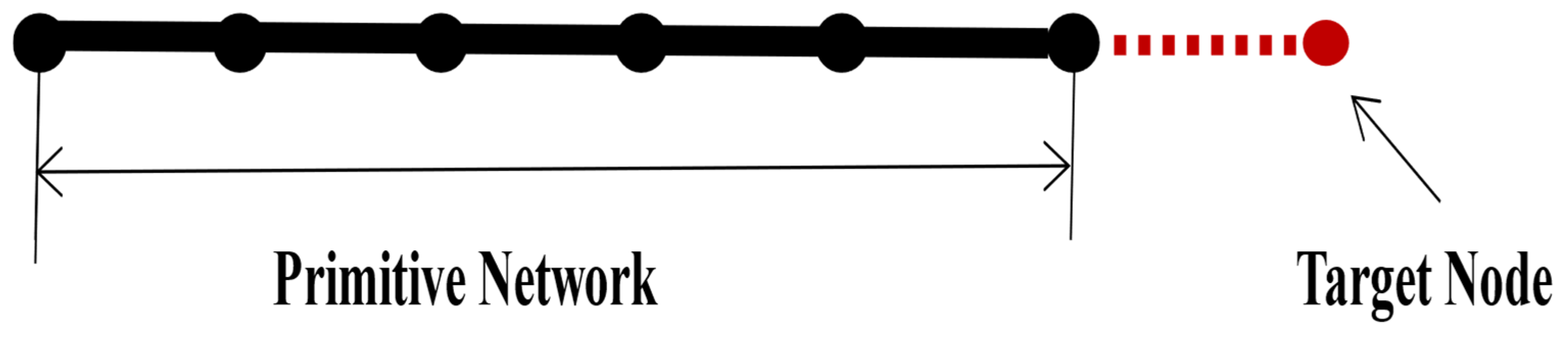
Output Prediction Values: Based on the predicted target node and the similarity to other nodes, the node with the highest similarity, denoted as ( t n * , y n * ), is added to the network. In this process, one edge is connected to the last node in the network (as adjacent nodes are connected in the visual graph algorithm). In Figure 6, as shown by the red dashed line, the target node is linked to the last node to be incorporated into the network. Another edge links the node ( t n * , y n * ) to the node. For example, in Figure 7, the 3rd node (highest similarity node) is linked to the 6th node via the red dashed line, and the green solid line indicates that the 7th node is determined by the 3rd and 6th nodes (adjacent nodes). To avoid using nodes that could produce inaccurate estimations, the nodes with the highest similarity are selected to anticipate future throughput [28]. Time series ( t n + 1 , y n + 1 ) are predicted using Equation (35) and are then compared with other algorithms.
y ^ n + 1 = y n y n * t n t n * t n + 1 t n + y n

4. Empirical

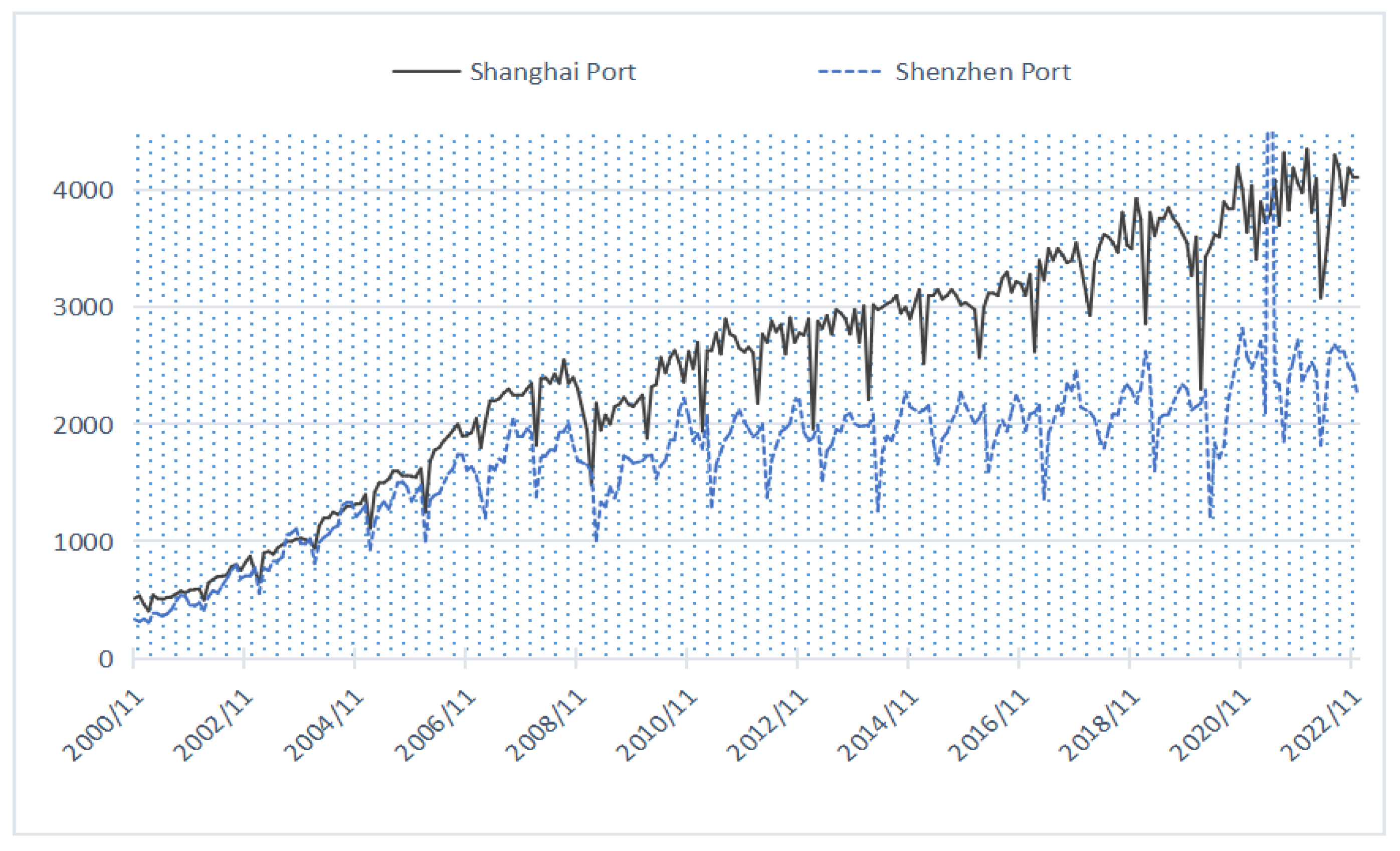
4.1. Data Description

This study selects Shanghai Port and Shenzhen Port as research subjects to validate the effectiveness of the proposed framework. Shanghai Port is situated at the meeting point of the Yangtze River and the East China Sea in the center of China’s coastline. It has historically been a vital hub for China’s foreign trade and transportation. As the largest port in the world in terms of container throughput and cargo volume, Shanghai Port holds a critical position in the international logistics system. Shenzhen Port, situated in the southern part of the Pearl River Delta and adjacent to Hong Kong, is a natural deep-water harbor in South China. Located in the developed Pearl River Delta region and close to international shipping routes, it serves as a crucial hub in China’s transportation network and holds significant international strategic importance. Based on this, this paper selects the time series data for container throughput for Shanghai Port from November 2000 to December 2022 and for Shenzhen Port from November 2000 to February 2023 for forecasting (Figure 8). For the Shanghai Port and Shenzhen Port container throughput datasets used in this paper, 90% of the samples from each dataset were selected as training samples, and the remaining 10% of the samples were used as test samples. This is done to validate the effectiveness of the hybrid prediction model combining complex networks, link prediction, and artificial intelligence methods in the prediction of container throughput in Chinese ports.

4.2. Experimental Setup

The foundational experimental setup was as follows: The hardware consists of an AMD Ryzen 7 (2.0 GHz) CPU with 16 GB of RAM. The software environment is based on a 64-bit Windows 11 OS, with algorithms implemented in Python 3.9. Key third-party libraries used include Tensorflow for scientific computation, numpy and pandas for data handling, pymrmr for feature selection, and networks for network structure analysis. The experimental parameter configuration employs three models for forecasting. The DNN model features a three-layer structure with ReLU-activated input and hidden layers and a sigmoid-activated output neuron. The LSTM model, addressing time series data via time-delay embedding, considers temporal data characteristics. Lastly, the SVM model with a linear kernel and probability estimates focuses on predictive confidence. These models aim to optimize predictive performance.

4.3. Performance Metrics

Making predictions about possible edges or connections that might emerge in a graph in the future is the challenge of link prediction. A U C (Area Under Curve) and P r e c i s i o n [29] are the two main measures used to assess how good the link prediction is.
To assess the quality of the link prediction categorization, the area under the ROC curve is computed ( A U C metric). It offers a general indicator of link prediction algorithms’ accuracy. In link prediction, two cases are considered: one from the test set E p and the other from the set of unlinked edges U E . Using the link prediction algorithm, the similarities of these edges are calculated and compared. There are two possible scenarios: in the first case, if the former similarity score is greater than the latter, a score of 1 is assigned; in the second case, if the two scores are equal, a score of 0.5 is assigned. It is defined as follows:
A U C = n + 0.5 n n
where n represents the number of independent comparisons, n is the quantity of times the first scenario occurs, and n is the quantity of times the second scenario occurs. A higher A U C value, closer to 1, suggests that the algorithm’s prediction accuracy is higher.
The P r e c i s i o n metric measures the precision of the algorithm on a local level. It considers only the ratio of accurately predicted edges among the top L predicted edges based on similarity scores. This metric can be expressed as follows:
P r e c i s i o n = N L
where N represents the number of edges appearing within the test collection E P among the top L edges ranked by prediction scores. An algorithm with a higher P r e c i s i o n value is predicted to be more accurate.
Additionally, to evaluate the error between time series predicted values and actual values, three error measurement metrics will be used: Mean Absolute Percentage Error ( M A P E ), Mean Absolute Error ( M A E ), and Root Mean Square Error ( R M S E ). These metrics are calculated using the following formulas:
M A P E = 1 N t = 1 N Y ^ t Y t Y t × 100
M A E = 1 N t = 1 N Y ^ t Y t
R M S E = 1 N t = 1 N Y ^ t Y t 2
where Y ^ t represents the predicted value of container throughput and Y t is the actual value of container throughput. Smaller values of MAPE, MAE, or RMSE show improved methodic prediction performance.

4.4. Results and Analysis

4.4.1. Construction of Container Throughput Time Series Network

Using a visual graph method, we first converted the time series data for Shanghai Port and Shenzhen Port into visual graphs, as seen in Figure 9 and Figure 10, respectively.
The network’s visual graphs give a clear picture of how connected each node is to every other node overall. This study computed certain common topological properties of the pictured networks to acquire more topological information about the visualized networks. Table 1 summarizes the results. The average degree and average clustering coefficient of nodes in the pictured network of Shenzhen Port’s container throughput are higher than those of Shanghai Port’s visualized network, according to a comparison of the topological attribute values in the table for the two ports. Shanghai Port’s network visualization, however, has a larger circumference than Shenzhen Port’s. It can be deduced from the values of these network topological properties that both.

4.4.2. Link Prediction Dataset Splitting

In this paper, we forecast links using artificial intelligence algorithms. It is crucial to evaluate how various link training set ratios affect the link prediction job before training the models.
Typically, link prediction can be treated as a single classification issue in supervised learning, for which our goal is to obtain positive samples representing links that exist in the network and negative samples representing links that do not exist. Let v x and v y be nodes in the graph G V , E . If there is a link between nodes v x and v y , they are labeled as positive samples in the link prediction task with a label of 1. If there is no link between v x and v y , they are labeled as negative samples in the link prediction task with a label of 0. Therefore, considering l x , y as the label for node pairs ( v x , v y ), l x , y can be divided into two classes of labels, defined as shown in Equation (41).
l x , y = 1 , v x , v y E 0 , v x , v y E
To comprehensively evaluate the model’s performance, following the standard practice for training link prediction, this study divided the link prediction dataset using a random sampling algorithm. This algorithm ensures that the probability of each link being included in the training and testing datasets is equal. Random sampling partition ratios of p = 0.1, p = 0.2, and p = 0.3 were employed. Specifically, for a network G containing N nodes and M edges, p M edges were randomly selected from the network to form the testing set, while the remaining (1– p M ) edges constituted the training set. Given that reducing the training set ratio further would result in poor connectivity between nodes and a lack of essential link information for prediction, smaller training set ratios were not considered. Subsequently, SVM, DNN, and LSTM models were separately employed for link prediction to assess their performance under different training set ratios. The average prediction accuracy in terms of A U C and P r e c i s i o n values for each prediction model was obtained by repeating the aforementioned experimental process, and Table 2 displays the test findings. It was noted that increasing the training set ratio from 70% to 90% resulted in improved A U C and Precision for all prediction models, as more unknown links were involved in the computation. To make sure the model is stable and reliable, all subsequent analyses were based on a training set ratio of 90% of the network’s links.

4.4.3. Path Information Order Determination and Feature Selection Analysis

One important task in link prediction research is figuring out the path information’s order. This research considers the influence of both first-order and second-order path information on node similarity when computing network similarity measures. In particular, the value of α in Equation represents the impact of second-order path information (19).
Since the α value directly affects the model’s prediction accuracy, to determine the appropriate α value, different α values are selected with a step size of 0.1. The selected metrics based on mRMR are used for prediction, and the corresponding prediction evaluation standard A U C values are calculated. To illustrate the effectiveness of feature selection based on mRMR, this paper compares it with 13 single features, including CN, Jaccard, AA, RA, PA, HPI, FL, LRW, SRW, Katz, LHNII, ACT, and MFI. Figure 11 and Figure 12 show the mRMR-based approach at different α values for Shanghai Port and Shenzhen Port, as well as the model’s average prediction accuracy ( A U C ) values for various kinds of single metrics.”
(1)
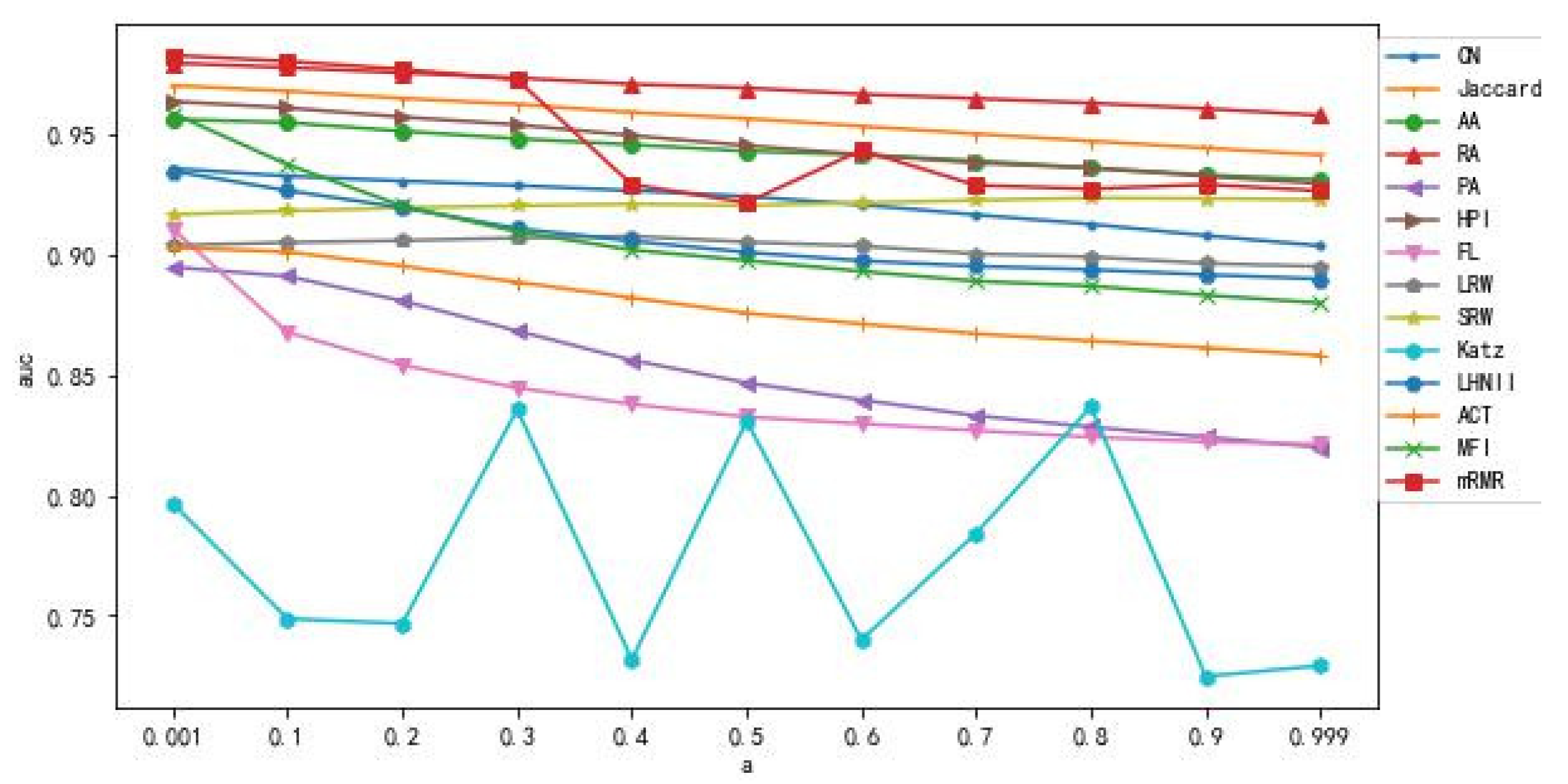
From Figure 11 and Figure 12, it can be observed that in the Shanghai Port dataset, predictive models using single metrics (such as RA, Jaccard, HPI, and AA) perform well, and the A U C values remain stable with changes in α . The Katz metric exhibits significant fluctuations in A U C values with changes in α, reaching its maximum when α = 0.8. Except for the SRW metric, the A U C values of other metrics show a decreasing trend as α increases. However, in the Shenzhen Port dataset, there is relatively larger variability in the overall feature performance compared to the Shanghai Port dataset, especially in that the LRW, SRW, FL, ACT, and CN metrics show a sharp decline after α = 0.1. Additionally, it can be observed that for some single metric algorithms with good predictive accuracy (such as RA), the performance improvement of models based on mRMR feature selection is not significant, and may even have a negative or near-zero improvement. This is because these algorithms already have a good definition of network structural information, providing high predictive accuracy. However, for algorithms with lower predictive performance (such as KATZ, HPI, FL) models based on mRMR feature selection can provide more structural information about similarity measures, resulting in better performance in predictions. In conclusion, with α = 0.1 and 90% of the network’s links serving as the training set, the predictive performance of the mRMR-based feature selection model is ideal;
(2)
The different values of α not only affect the choice of similarity feature metrics but also influence the overall model performance. From Figure 11 and Figure 12, we can observe that as α values get closer to 0, the A U C values become higher. In the Shanghai Port dataset, the features selected based on mRMR are primarily dominated by global information-based metrics like LNHII and ACT, as well as semi-local metrics like SRW and FL. In the Shenzhen Port dataset, the features selected by mRMR are mainly based on global information, particularly LNHII, and semi-local information, particularly FL features. In both datasets, measures based on local information like CN, RA, PA, and Jaccard appear very infrequently, indicating that, in the chosen dataset networks and constructed prediction models in this study, similarity metrics based on global and semi-local information provide better quantification of network properties;
(3)
From Figure 11 and Figure 12, it can be observed that as α increases, the change in A U C values for various feature algorithms does not strictly exhibit a decreasing trend. The relationship between the adjustable parameter α and A U C differs slightly for the two networks in this research. The link prediction accuracy of the suggested technique is better for networks with comparatively high average clustering coefficients. The significant fluctuation in the α parameter for the Shenzhen Port network is due to its inherent characteristics, making second-order path information crucial for prediction. In denser networks, second-order path information has a more significant impact. However, the fluctuation in the curve shown in Figure 12 does not directly correlate with the network’s average clustering coefficient. Despite the Shanghai Port visual network’s comparatively high average clustering coefficient, the consideration of second-order path information has a less noticeable impact on it. This suggests that second-order path information has limitations for certain networks and cannot cover all the relevant information.
Table 3 and Table 4 present the selected features and the A U C values for the link prediction models for the Shanghai Port and Shenzhen Port datasets, respectively, at different α values.
From Table 3 and Table 4, it can be observed that for both the Shanghai Port and Shenzhen Port datasets, the combination of similarity metrics selected by mRMR, including “AA, MFI, SRW, ACT” and “LRW, FL, LHNII, Jaccard,” with α   = 0.1, yielded the highest A U C scores for the three models (SVM, DNN, and LSTM). For the Shanghai Port dataset, the AUC scores were 0.9807, 0.9716, and 0.9494, respectively, while for the Shenzhen Port dataset, the A U C scores were 0.9997, 0.9997, and 1.0000, respectively. Therefore, it is considered that this combination scheme with α = 0.1, utilizing the features selected by mRMR (AA, MFI, SRW, ACT, LRW, FL, LHNII, Jaccard) for similarity metric computation, exhibits superior accuracy and ensures good link prediction performance for the algorithm models.

4.4.4. Different Prediction Model Comparison Analysis

To validate the reliability and sustainability of the hybrid forecasting model proposed in this work, which combines complex network analysis, link prediction, and artificial intelligence algorithms, it is contrasted with baseline forecasting methods and hybrid forecasting methods built on first-order path information. The models included in the comparison are as follows: (1) Three baseline prediction models, including SVM, DNN, and LSTM; (2) three prediction models that consider only first-order path information and feature selection based on the baseline models, including CN1-SVM, CN1-DNN, and CN1-LSTM; and (3) three hybrid link prediction models that consider both first-order and second-order path information as well as feature selection, representing the models under the prediction framework proposed in this paper, including CN2-SVM, CN2-DNN, and CN2-LSTM. Table 5 compares the predictive performance of these nine models.
From Table 5, it can be observed that for both the Shanghai Port and Shenzhen Port visual networks, the algorithm proposed in this paper, which combines first-order and second-order path information from complex networks and employs mRMR feature selection, outperforms the comparative models. This demonstrates the effectiveness of incorporating second-order path information and using mRMR feature selection in conjunction with artificial intelligence models for link prediction.
Furthermore, the RMSE, MAPE, and MAE values for CN2-SVM, CN2-DNN, CN2-LSTM, CN1-SVM, CN1-DNN, and CN1-LSTM are significantly lower than those for the corresponding SVM, DNN, and LSTM models, indicating that the hybrid models have better performance and predictive accuracy than the baseline models. Specifically, in the Shanghai Port dataset, CN2-SVM, CN2-DNN, CN2-LSTM, and CN1-LSTM perform the best, with identical RMSE, MAPE, and MAE values of 72.25, 0.020, and 46.13, respectively. This similarity is because these four models obtain the same first-order and second-order path target nodes and identify the highest similarity nodes during the regression of throughput values. Following them, the first-order path models CN1-SVM and CN1-DNN perform slightly worse, while the baseline models SVM, DNN, and LSTM exhibit the poorest performance. Similarly, in the Shenzhen Port dataset, except for the slightly higher RMSE value of CN2-LSTM compared to the first-order path RMSE value, overall, models based on network second-order path information exhibit the best predictive performance, followed by models based on network first-order path information, while the baseline models SVM, DNN, and LSTM perform the worst.
The preceding investigation indicates that complex network-based time series forecasting performs better than baseline models. There are two reasons for this: Initially, time series data and complex networks are closely related because time series information may be captured by networks, which enables the network to acquire the time series’ characteristics. One unique kind of data structure that tracks the dynamic changes of continuous complex network data structures over an ongoing period is the complex network time series. The intricate network structure displays distinct connection interactions at every independent time point. This complex network structure shows regular evolution characteristics from a temporal perspective, and in certain ways, with a suitable analysis, complex networks can be predicted. Furthermore, the integration of first-order path data with second-order.

5. Conclusions

This research contributes to the field of systems analysis by offering a novel approach to the development and protection of national port resources, focusing on the prediction of port container throughput. Recognizing the systemic nature of ports as part of larger economic and regulatory environments, our approach addresses the challenges posed by the time series of port container throughput, which exhibits complex and nonlinear characteristics due to seasonal variations, hinterland economic activities, and regulatory frameworks. From a systems perspective, we first convert the throughput time series through a complicated network using a visual graph algorithm. This allows us to capture the first-order and second-order path information of the network, reflecting the systemic interactions and dependencies within port operations. We then introduce 13 similarity metrics, derived from local, semi-local, and global network structural similarities, to form a comprehensive feature set that encapsulates various aspects of the complex network system. Employing the mRMR method, we decide which features are best for the network, illustrating systems theory’s principles of efficiency and efficacy. These features are then used as inputs for three advanced artificial intelligence models SVM, DNN, and LSTM to perform link prediction. This step is crucial for understanding and forecasting the systemic behavior of port logistics. The final stage involves regression analysis to predict container throughput values, a key performance indicator in port systems management. Test findings show that our suggested approach can somewhat accurately anticipate port container throughput. When compared to baseline models like DNN, SVM, and LSTM, our model, which integrates complex networks and link prediction, shows reduced prediction errors. This indicates a significant advancement in system-oriented predictive modeling for port container throughput, contributing valuable insights to the field of systems analysis and management.
This study is not merely an application case for specific ports but also offers a new theoretical perspective by integrating complex network theory with time series analysis to understand and predict the dynamic behavior of complex systems. The methodological innovation of this approach provides novel analytical tools and perspectives for systems theory, particularly in understanding complex, interdependent system structures. Integrating these methods into a unified framework offers a comprehensive model for systems analysis, representing a relatively novel endeavor. Through the combined application of these methods, we have not only improved the accuracy of port operation forecasts but also enriched the toolkit for systems analysis, which is immensely valuable for management and decision-making. This interdisciplinary approach can be widely applied to various types of complex systems, thereby advancing the development of the entire field of systems analysis.
Although the proposed prediction approach performs well, it can still be improved. For example, our forecasting model is built on an unweighted, undirected static network and overlooks the directionality and significance of links. Given that many real networks are directed, weighted, and constantly changing, future research may concentrate on improving the proposed technique for forecasting in directed, weighted, and dynamic networks.

Author Contributions

Conceptualization, X.L., Y.W. and M.Y.; methodology, Y.W.; software, Y.W.; validation, X.L. and Y.W.; formal analysis, X.L. and M.Y.; investigation, M.Y.; data curation, Y.W.; writing—original draft preparation, Y.W.; writing—review and editing, X.L. and M.Y.; visualization, Y.W.; supervision, X.L. and M.Y. All authors have read and agreed to the published version of the manuscript.

Funding

This research was funded by the National Natural Science Foundation of China, grant numbers [71701122, 11801352].

Data Availability Statement

Data are contained within the article.

Conflicts of Interest

The authors declare no conflict of interest.

References

  1. Du, D.; Liu, T.; Guo, C. Analysis of Container Terminal Handling System Based on Petri Net and ExtendSim. Promet-Traffic Transp. 2023, 35, 87–105. [Google Scholar] [CrossRef]
  2. Singh, S.N.; Mohapatra, A. Repeated Wavelet Transform Based ARIMA Model for Very Short-Term Wind Speed Forecasting. Renew. Energy 2019, 136, 758–768. [Google Scholar]
  3. Wang, J.; Niu, X.; Liu, Z.; Zhang, L. Analysis of the Influence of International Benchmark Oil Price on China’s Real Exchange Rate Forecasting. Eng. Appl. Artif. Intell. 2020, 94, 103783. [Google Scholar] [CrossRef]
  4. Du, P.; Wang, J.; Hao, Y.; Niu, T.; Yang, W. A Novel Hybrid Model Based on Multi-objective Harris Hawks Optimization Algorithm for Daily PM2.5 and PM10 Forecasting. Appl. Soft Comput. 2020, 96, 106620. [Google Scholar] [CrossRef]
  5. Fan, Y.Y.; Yu, S.Q. Port Container Throughput Forecast Based on NARX Neural Network. J. Shanghai Marit. Univ. 2015, 1636, 012024. [Google Scholar]
  6. Huang, A.; Lai, K.; Li, Y.; Wang, S. Forecasting Container Throughput of Qingdao Port with a Hybrid Model. J. Syst. Sci. Complex. 2015, 28, 105–121. [Google Scholar] [CrossRef]
  7. Lacasa, L. From Time Series to Complex Networks: The Visibility Graph. Proc. Natl. Acad. Sci. USA 2008, 105, 4972–4975. [Google Scholar] [CrossRef]
  8. Zhou, T.; Jin, N. Time Series Network Model Based on Finite Traversal Visual Graph. Acta Phys. Sin. 2012, 61, 86–96. [Google Scholar]
  9. Ma, Z. Identification of Complex Network for ECG Signals of Healthy and Myocardial Infarction Patients Based on Multichannel Visual Graphs. Acta Phys. Sin. 2022, 71, 48–57. [Google Scholar] [CrossRef]
  10. He, Y.; Liu, J.N.K.; Hu, Y.; Wang, X.-Z. OWA Operator Based Link Prediction Ensemble for Social Network. Expert Syst. Appl. 2015, 42, 21–50. [Google Scholar] [CrossRef]
  11. Zhang, Q.; Tong, T.; Wu, S. Hybrid Link Prediction via Model Averaging. Phys. A 2020, 556, 124772. [Google Scholar] [CrossRef]
  12. Ayoub, J.; Lotfi, D.; Marraki, M.E.; Hammouch, A. Accurate Link Prediction Method Based on Path Length Between a Pair of Unlinked Nodes and Their Degree. Soc. Netw. Anal. Min. 2020, 10, 1–13. [Google Scholar] [CrossRef]
  13. Güneş, İ.; Gündüz-Öğüdücü, Ş.; Çataltepe, Z. Link Prediction Using Time Series of Neighborhood-Based Node Similarity Scores. Data Min. Knowl. Discov. 2016, 30, 147–180. [Google Scholar] [CrossRef]
  14. Agarwal, A.; Marwan, N.; Maheswaran, R.; Merz, B.; Kurths, J. Quantifying the Roles of Single Stations within Homogeneous Regions Using Complex Network Analysis. J. Hydrol. 2018, 563, 802–810. [Google Scholar] [CrossRef]
  15. Liben-Nowell, D.; Kleinberg, J. The Link Prediction Problem for Social Networks. In Proceedings of the Twelfth International Conference on Information and Knowledge Management, New Orleans, LA, USA, 3–8 November 2003; pp. 556–559. [Google Scholar]
  16. Adamic, L.A.; Adar, E. Friends and Neighbors on the Web. Soc. Netw. 2003, 25, 211–230. [Google Scholar] [CrossRef]
  17. Zhou, T.; Lü, L.; Zhang, Y.C. Predicting Missing Links via Local Information. Eur. Phys. J. B 2009, 71, 623–630. [Google Scholar] [CrossRef]
  18. Barabási, A.L.; Albert, R. Emergence of Scaling in Random Networks. Science 1999, 286, 509–512. [Google Scholar] [CrossRef]
  19. Jaccard, P. Etude Comparative de la Distribution Florale dans une Portion des Alpes et des Jura. Bull. Soc. Vaud. Sci. Nat. 1901, 37, 547–579. [Google Scholar]
  20. Ravasz, E.; Somera, A.L.; Mongru, D.A.; Oltvai, Z.N.; Barabasi, A.-L. Hierarchical Organization of Modularity in Metabolic Networks. Science 2002, 297, 1551–1555. [Google Scholar] [CrossRef]
  21. Liu, W.; Lü, L. Link Prediction Based on Local Random Walk. Europhys. Lett. 2010, 89, 58007. [Google Scholar] [CrossRef]
  22. Papadimitriou, A.; Symeonidis, P.; Manolopoulos, Y. Fast and Accurate Link Prediction in Social Networking Systems. J. Syst. Softw. 2012, 85, 2119–2132. [Google Scholar] [CrossRef]
  23. Katz, L. A New Status Index Derived from Sociometric Analysis. Psychometrika 1953, 18, 39–43. [Google Scholar] [CrossRef]
  24. Guo, J.; Meng, Y.Y. A Link Prediction Algorithm Using Relative Entropy to Measure Node Structural Similarity. J. Lanzhou Jiaotong Univ. 2022, 1955, 012078. [Google Scholar]
  25. Abdourahamane, Z.S.; Acar, R.; Serkan, Ş. Wavelet–Copula-Based Mutual Information for Rainfall Forecasting Applications. Hydrol. Process. 2019, 33, 1127–1142. [Google Scholar] [CrossRef]
  26. Cortes, C.; Vapnik, V. Support-Vector Networks. Mach. Learn. 1995, 20, 273–297. [Google Scholar] [CrossRef]
  27. Schmidhuber, J.; Hochreiter, S. Long Short-Term Memory. Neural Comput. 1997, 9, 1735–1780. [Google Scholar]
  28. Zhang, R.; Ashuri, B.; Shyr, Y.; Deng, Y. Forecasting Construction Cost Index Based on Visibility Graph: A Network Approach. Phys. A Stat. Mech. Its Appl. 2018, 493, 239–252. [Google Scholar] [CrossRef]
  29. Lü, L.Y. Link Prediction in Complex Networks. J. Univ. Electron. Sci. Tech. China 2010, 39, 651–661. [Google Scholar]
Figure 1. Diagram Illustrating Link Prediction Problem.
Systems 12 00023 g001
Figure 2. First-Order Path Information and Second-Order Path Information in Networks.
Systems 12 00023 g002
Figure 3. LSTM Architecture Diagram.
Systems 12 00023 g003
Figure 4. DNN Architecture Diagram.
Systems 12 00023 g004
Figure 5. Research Framework Diagram.
Systems 12 00023 g005
Figure 6. The Addition of Target Nodes.
Systems 12 00023 g006
Figure 7. Link Prediction Node Linkage Schematic Diagram.
Systems 12 00023 g007
Figure 8. Container Throughput at Shanghai Port and Shenzhen Port (Unit: Thousand TEUs).
Systems 12 00023 g008
Figure 9. Shanghai Port Visual Network Diagram.
Systems 12 00023 g009
Figure 10. Shenzhen Port Visual Network Diagram.
Systems 12 00023 g010
Figure 11. The Average Predictive Accuracy A U C Values of Models for Various Feature Indicators at Different α Values in Shanghai Port. a = α.
Systems 12 00023 g011
Figure 12. The Average Predictive Accuracy A U C Values of Models for Various Feature Indicators at Different α Values in Shenzhen Port. a = α.
Systems 12 00023 g012
Table 1. Dataset Network Topology Parameters.
PortNodes Number
N
Edges Number
M
Average Degree
<k>
Average Clustering Coefficient <c>Path Length
<d>
Shanghai Port2619547.310.73710
Shenzhen Port2639717.380.7526
Table 2. Evaluation Scores for Different Partition Ratios of Link Prediction Datasets.
PortModel7:38:29:1
A U C P r e c i s i o n A U C P r e c i s i o n A U C P r e c i s i o n
Shanghai PortSVM0.9650.8590.9680.8490.9810.857
DNN0.9360.8560.9440.8490.9550.857
LSTM0.9380.8560.9350.8450.9440.857
Shenzhen PortSVM0.9940.9630.9940.9700.9990.989
DNN0.9940.9630.9950.9691.0000.990
LSTM0.9950.9630.9950.9691.0000.990
Table 3. The A U C Values of Selected Features and Link Prediction Models at Different α Values in Shanghai Port.
α Feature SelectionSVMDNNLSTM
0.1‘AA’, ‘MFI’, ‘SRW’, ‘ACT’0.98070.97160.9494
0.2‘AA’, ‘SRW’, ‘FL’, ‘ACT’0.97740.96530.9453
0.3‘AA’, ‘FL’, ‘ACT’, ‘LHNII’0.97300.96160.9474
0.4‘LRW’, ‘FL’, ‘LHNII’, ‘Katz’0.92310.93100.9289
0.5‘SRW’,’MFI’, ‘ACT’, ‘LHNII’0.90600.92060.9189
0.6‘SRW’, ‘FL’, ‘ACT’, ‘LHNII’0.92500.93340.9226
0.7‘SRW’, ‘FL’, ‘ACT’, ‘LHNII’0.92640.93440.9248
0.8‘SRW’, ‘FL’, ‘ACT’, ‘LHNII’0.92760.93790.9243
0.9‘LRW’, ‘FL’, ‘LHNII’, ‘Katz’0.92440.92600.9272
Table 4. The A U C Values of Selected Features and Link Prediction Models at Different α Values in Shenzhen Port.
α Feature SelectionSVMDNNLSTM
0.1‘LRW’, ‘FL’, ‘LHNII’, ‘Jaccard’0.99970.99971.0000
0.2‘LRW’, ‘FL’, ‘ACT’, ‘LHNII’0.99400.99010.9843
0.3‘LRW’, ‘FL’, ‘LHNII’, ‘Katz’0.98050.97070.9599
0.4‘AA’, ‘PA’, ‘LHNII’, ‘HPI’0.99010.98900.9856
0.5‘LRW’, ‘FL’, ‘ACT’, ‘LHNII’0.98760.97180.9568
0.6‘LRW’, ‘FL’, ‘LHNII’, ‘SRW’0.98780.98310.9725
0.7‘SRW’, ‘FL’, ‘ACT’, ‘LHNII’0.95450.98100.9782
0.8‘SRW’, ‘MFI’, ‘ACT’, ‘Katz’0.98710.98740.9890
0.9‘SRW’, ‘FL’, ‘ACT’, ‘LHNII’0.95490.93850.9549
Table 5. Comparison of Results from Different Forecasting Models for Shanghai Port and Shenzhen Port.
Shanghai PortShenzhen Port
RMSEMAPEMAERMSEMAPEMAE
SVM261.380.110208.07424.920.242298.54
DNN248.610.070163.85382.720.109193.51
LSTM243.090.077174.42387.320.108178.32
CN1-SVM104.380.02864.73107.460.03458.72
CN1-DNN74.210.02047.09110.490.03763.40
CN1-LSTM72.250.02046.13110.260.03662.69
CN2-SVM72.250.02046.13107.460.03458.72
CN2-DNN72.250.02046.13109.980.03662.45
CN2-LSTM72.250.02046.13117.620.03561.17
Disclaimer/Publisher’s Note: The statements, opinions and data contained in all publications are solely those of the individual author(s) and contributor(s) and not of MDPI and/or the editor(s). MDPI and/or the editor(s) disclaim responsibility for any injury to people or property resulting from any ideas, methods, instructions or products referred to in the content.

