

Deep Reinforcement Learning Reward Function Design for Autonomous Driving in Lane-Free Traffic
by
 , , and
Athanasia Karalakou
1,†,
Dimitrios Troullinos
2,*,†,
Georgios Chalkiadakis
1 and
Markos Papageorgiou
2 1
School of Electrical and Computer Engineering, Technical University of Crete, 73100 Chania, Greece
2
School of Production Engineering and Management, Technical University of Crete, 73100 Chania, Greece
*
Author to whom correspondence should be addressed.
†
These authors contributed equally to this work.
Systems 2023, 11(3), 134; https://doi.org/10.3390/systems11030134
Submission received: 30 January 2023
/
Revised: 25 February 2023
/
Accepted: 28 February 2023
/
Published: 2 March 2023
(This article belongs to the Special Issue Advancements in the Practical Applications of Agents, Multi-Agent Systems and Simulating Complex Systems)
Abstract
:Lane-free traffic is a novel research domain, in which vehicles no longer adhere to the notion of lanes, and consider the whole lateral space within the road boundaries. This constitutes an entirely different problem domain for autonomous driving compared to lane-based traffic, as there is no leader vehicle or lane-changing operation. Therefore, the observations of the vehicles need to properly accommodate the lane-free environment without carrying over bias from lane-based approaches. The recent successes of deep reinforcement learning (DRL) for lane-based approaches, along with emerging work for lane-free traffic environments, render DRL for lane-free traffic an interesting endeavor to investigate. In this paper, we provide an extensive look at the DRL formulation, focusing on the reward function of a lane-free autonomous driving agent. Our main interest is designing an effective reward function, as the reward model is crucial in determining the overall efficiency of the resulting policy. Specifically, we construct different components of reward functions tied to the environment at various levels of information. Then, we combine and collate the aforementioned components, and focus on attaining a reward function that results in a policy that manages to both reduce the collisions among vehicles and address their requirement of maintaining a desired speed. Additionally, we employ two popular DRL algorithms—namely, deep Q-networks (enhanced with some commonly used extensions), and deep deterministic policy gradient (DDPG), which results in better policies. Our experiments provide a thorough investigative study on the effectiveness of different combinations among the various reward components we propose, and confirm that our DRL-employing autonomous vehicle is able to gradually learn effective policies in environments with varying levels of difficulty, especially when all of the proposed rewards components are properly combined.
1. Introduction
Applications of reinforcement learning (RL) in the field of autonomous driving have been gaining momentum in recent years [1] due to advancements in Deep RL [2,3], giving rise to novel techniques [4]. The fact that deep reinforcement learning (DRL) can handle high dimensional state and action spaces makes it suitable for controlling autonomous vehicles. Another important reason for this momentum is increasing interest in autonomous vehicles (AVs), as the current and projected technological advancements in the automotive industry can enable such methodologies in the real world [5,6]. As a result, novel traffic flow research endeavors have already emerged, such as TrafficFluid [7], which primarily targets traffic environments with penetration of AVs (no human drivers). Trafficfluid examines traffic environments with two fundamental principles:
- (i) Lane-free vehicle movement, meaning that AVs under this paradigm do not consider lane-keeping, but are rather free to be located anywhere laterally. Lanes emerged to simplify human driving, and when only automated vehicles exist, they may no longer be required, given the observational capabilities of an AV compared to that of a human driver. The renunciation of the lane principle enables higher utilization of the available road capacity, and the lane-changing task is an operation that is no longer needed. AVs’ lateral positions can be regulated gradually in order to overtake, and in this manner, an AV can also accommodate upstream traffic via the second principle examined under the lane-free paradigm—that is,
- (ii) Nudging, where vehicles may adjust their behavior so as to assist vehicles on the back that attempt to overtake. In lane-based traffic, this would involve a lane-change operation, and as such, nudging could not actually be considered in conventional traffic. In contrast, in lane-free settings, a vehicle can provide the necessary space for receding vehicles just by leaning towards an appropriate lateral direction.
In the context of lane-free driving, multiple vehicle-movement strategies have already been proposed [7,8,9,10]. To be more specific, existing studies have focused on optimal control methods that involve model predictive control [9]. In addition, the application of a movement strategy based on heuristic rules that incorporates the notion of “forces” [7], along with an extension on this endeavor [11], provides empirical insight on the benefits of lane-free traffic. Moreover, authors of [10] have designed a two dimensional cruise controller that specifically addresses lane-free traffic environments, and the authors of [12] incorporated these controllers in a quite challenging roundabout scenario, and provided an experimental microscopic study. Finally, ref. [8] investigated the utilization of the max-plus algorithm, and constructed a dynamic graph structure of the vehicles, considering communication among vehicles as well.
However, to the best of our knowledge, while there is an abundance of (deep) RL applications for conventional (lane-based) traffic environments [1,4,5], so far only two papers in the literature [13,14] tackle the problem of lane-free traffic with RL techniques. We believe that (deep) RL could be a valuable asset for managing this novel challenging domain, as it is capable of solving complex and multi-dimensional tasks with lower prior knowledge because of its ability to learn different levels of abstractions from data. Furthermore, (deep) RL provides policies that automatically adjust to the environment, and thus there is no need for either a centralized authority or explicit communication among vehicles. The efficiency of RL heavily relies on the design of the Markov decision process, and especially on the reward function guiding the agent’s learning. The reward design is crucial and determines the overall efficiency of the resulting policy. This is evident in DRL studies related to AVs [5].
Against this background, in this work we tackle the problem of designing an RL agent that learns a vehicle-movement strategy in lane-free traffic environments. To this end, we establish a Markov decision process (MDP) for lane-free autonomous driving, given a single agent environment populated with other vehicles adopting a rule-based lane-free driving strategy [7], primarily focusing on the design of the reward function. Given the nature of the DRL algorithms, their ability to properly learn only with delayed rewards and obtain a (near-) optimal policy is uncertain, so we propose a set of different reward components, ranging from delayed rewards to more elaborate and therefore, more informative regarding the problem’s objectives. The learning objectives in our environment are twofold, as they address: (i) safety, i.e., collision avoidance among vehicles; and (ii) desired speed, i.e., that our agent attempts to maintain a specific speed of choice.
In a nutshell, the main contributions of this work are the following:
- We constructed different components of reward functions specifically tied to a the lane-free traffic environment at various levels of information;
- We then combined and collated the aforementioned components, in order to attain an efficient reward function;
- We experimentally investigated the effectiveness of different combinations of the various reward components we propose, using the deep deterministic policy gradient algorithm;
- We confirmed experimentally that our DRL-employing autonomous vehicle is able to gradually learn effective policies;
- Finally, we conducted a comparative experimental study between several well- established deep Q-network variants, and the deep deterministic policy gradient algorithm.
This paper constitutes an extension of our work in [13], appearing in the Proceedings of the 20th International Conference on Practical Applications of Agents and Multi-Agent Systems (PAAMS 2022). Several contributions are distinct in this paper, compared to those already in [13], namely:
- We put forward a novel reward component that can guide the vehicle in a lateral placement appropriate for overtaking, along with a related experimental evaluation;
- We showcase experimentally that the inclusion of this new component in the reward function yields superior results, especially for high traffic densities;
- Our experimental evaluation was under more intense traffic conditions than those examined in [13], with various densities of nearby vehicles;
- As mentioned above, we conducted a comparative study between DDPG and DQN variants, the results of which point to DDPG exhibiting superior performance, and as such constituting a suitable choice for training an agent via DRL in this complex, continuous domain.
The rest of this paper is structured as follows: In Section 2, we discuss the relevant background and related work, and in Section 3 we present the proposed approach in detail. Then, in Section 4 we provide a detailed experimental evaluation. Finally, in Section 5 we summarize our study and discuss future work.
2. Background and Related Work
In this section, we discuss the theoretical background of this work and provide further information about related work.
2.1. Markov Decision Process
A Markov decision process (MDP) [15] is a mathematical framework that completely describes the environment in a reinforcement learning problem, and they are fundamental for decision-making problems. An MDP can be defined by the 5-tuple:
where S describes the state space, A denotes the action space, P describes the transition model, R refers to the reward model, and is the discount factor.
2.2. Deep Q-Networks and Extensions
A deep Q-network (DQN) [2] adopts the Q-learning algorithm [16,17,18] for function approximation using neural networks, utilizes convolutional neural networks to obtain a graphical representation of the input state for an environment, and produces a vector of Q-values associated with each possible action. The concepts of target network and experience replay, formally introduced in [2], are the primary methods that enable the use of deep learning for approximating Q functions, resolving the issues of network stability. The Q-network is updated according to the following loss function:
where refers to the Q-network’s target value at iteration t, and and are the network’s parameters at iteration t and at a previous iteration, respectively—the latter being the target network’s parameters.
The main idea of experience replay is to store the agent’s experiences (the tuples ) in a buffer. Then, in each training step, a batch of experiences is uniformly sampled from the buffer and fed to the network for training. Experience replay ensures that old experiences are not disregarded in later iterations, and removes the correlations in the data sequences, feeding the network with independent data. This is suitable for DQN, since it is an off-policy method.
A well-known pathology of Q-learning, and consequently of DQN, is overestimation occurring from the use of the max operator in the Bellman equation to compute Q-values. The double deep Q-networks (DDQN) [19] algorithm addresses this issue by decomposing the maximizing operation in the target into action selection and evaluation. The idea behind the DDQN is that of double Q-learning [20], which includes two Q-functions. One function selects the optimal action, and the other estimates the value function. As a consequence, double DQN can offer faster training with better rewards across many domains, as evident by the results in [20]. Specifically, DDQN uses (as in vanilla DQN) the target network as the second action-value function, but it selects the next maximizing action according to the current network, while utilizing the target Q-network to calculate its value. The update is similar to DQN’s, but the target is replaced with:
Prioritized experience replay (PER) [21] is an additional DQN extension that focuses on prioritizing the experiences that contain more “important” information than others. Each experience is stored with an additional priority value, so that experiences with higher priority have a higher sampling probability and therefore, have the chance to remain longer in the buffer than others. As importance measure, the temporal difference (TD) error [18], can be used. It is expected that if the TD error is high (in absolute value), the agent can learn more from the corresponding experience because the agent behaved better or worse than expected.
The dueling network architecture (DNA) [22] decouples the value and advantage function [23], which leads to improved performance. In detail, it is constructed with two streams, one of them providing an estimate of the value function, and the other stream producing an estimate of the advantage function. There is a common feature learning module which is then separated to produce the two different mentioned outputs that are then combined appropriately in order to compute the state–action value function Q.
2.3. Deep Deterministic Policy Gradient
Deep deterministic policy gradient (DDPG) [24] is an off-policy, actor–critic algorithm that utilizes the deterministic policy gradient (DPG) [25] and the DQN architectures, and it overcomes the restriction of discrete actions.
It uses experience replay, just like a DQN, and target networks to compute the target y in the temporal difference error. To be more specific, target networks are two separate networks which are copies of the actor and critic network and are updated in a slow pace, in order to track the learned networks. The update for the critic is given by the standard DQN update by taking targets to be:
where and refer to the target networks for the critic and actor, respectively. The differentiating factor in the critic network architecture, with respect to DQN, is that the network contains the action vector as an input and has a single output approximating the corresponding Q-value. Moreover, the policy (actor network) in DDPG is updated using the sampled policy gradient, given a minibatch of transitions [25]:
where refers to the actor network with parameters , and N is the size of the sampled minibatch from the buffer. DDPG also introduces the notion of soft target updates to improve upon learning stability, meaning that the network parameters of the actor () and critic () are updated in every iteration through a temperature parameter as: , with .
2.4. Related Work
Under the lane-free traffic paradigm, multiple vehicle-movement strategies [7,8,9,10] have already been proposed, with approaches stemming from control theory, optimal control, and multi-agent decision making. In more detail, the authors of [7,11] introduced and then enhanced a lane-free vehicle-movement strategy based on heuristic rules that involve the notion of “forces” being applied to vehicles, in the sense that vehicles “push” one another so as to overtake, or in general to react appropriately. Then, reference [9] introduced a policy for lane-free vehicles based on optimal control methods and utilizing a model predictive control paradigm, where each vehicle optimizes its behavior for a specified future horizon, considering the trajectories of nearby vehicles as well. Furthermore, the authors of [10] designed a two-dimensional cruise controller for lane-free traffic, with more emphasis on control theory. They provided a mathematical framework for the controller design considering a continuous-time dynamical system for the kinetic motion and control of vehicles. Then, the authors of [12] incorporated a variation of this controller that is appropriate for discrete-time dynamical systems. The authors apply this in a challenging lane-free roundabout scenario populated with vehicles following different routing schemes within the roundabout. Finally, the authors of [8] tackled the problem with the use of the max-plus algorithm. The authors constructed a dynamic graph structure of the vehicles, considering communication among vehicles as well, and provided an extension in [26] for a novel dynamic discretization procedure and an updated formulation of the problem.
To the best of our knowledge, besides the conference paper [13] we extend herein, there is only one work in the literature that has tackled lane-free traffic using RL: In [14], the authors introduced a novel vehicle-movement strategy for lane-free environments that also incorporates DDPG for a learning agent in a lane-free environment. This agent learns to maintain an appropriate gap with a single vehicle downstream1 [14], and other operations are handled by different mechanisms based on the notion of repulsive forces and nudging, similarly to [7]. Notably, the overall implementation differed significantly with respect to our work, since the underlying endeavor was evidently quite distinct. The goal of this work was to investigate the use of RL for the task of lane-free driving, its potential, and limitations in this environment, by exclusively utilizing a relevant and well-studied DRL algorithm. Instead, the RL agent in [14] is part of a system composed of different controlling components. As such, in that case the learning task involves a specific longitudinal operation, where the agent also needs to learn to act in accordance with the other mechanisms.
Finally, there are several papers that report reward-function design for (deep or not, single- or multi-agent) RL techniques for lane-based traffic.
In the related literature, it is common to have a reward function form that contains multiple reward components (tied to different objectives), similarly to our approach. Regarding the total reward function that the agent receives, it is usually a simple weighted sum of the different reward components—whereas we employ a reciprocal form. In [27,28], the authors tackle a single-agent lane-based environment in a multi-lane highway using RL. These two approaches differ significantly in their MDP formulation and the RL algorithm of choice. However, they both contain a reward function comprised of several terms in an additive form. This aspect is apparent in multiagent RL applications as well. For instance, in [29], the authors examine a multiagent roundabout environment using the A3C method with parameter sharing among different learning agents. There, the agents likewise receive a reward as a sum of different reward terms tied to collision avoidance, maintaining an operational speed and terminal conditions. Finally, ref. [30] examines a signalized intersection environment with multiple vehicles learning to operate using the Q-learning algorithm in order to derive an efficient policy. Again, we observe the summation of different terms that form the total reward value that each agent receives.
3. Our Approach
In this section, we first present in detail the lane-free traffic environment we consider, and then the various features of the MDP formulation—specifically, the state representation, and the action space, and the different components proposed for the reward function design.
3.1. The Lane-Free Traffic Environment
Regarding the training environment, we consider a ring-road traffic scenario populated with numerous automated vehicles applying the lane-free driving behavior, as outlined in [7]. Our agent is an additional vehicle that adopts the proposed MDP formulation (more details in the next subsections), learning a policy through observation of the environment. The agent’s observational capabilities include the positions and speeds of nearby vehicles, and its own position and speed. Both the position and speed are observed as 2-dimensional vectors, consisting of the associated longitudinal (x axis) and lateral (y axis) values. All the surrounding vehicles share the same dimensions and movement dynamics. Each vehicle initially adopts a random desired speed , within a specified range (). Our agent controls two (continuous) variables, namely, the longitudinal and lateral acceleration values in m/s2, and determines the gas/break through , and left/right steering through .
Figure 1 depicts the traffic environment. A highway was used to simulate the scenario for the examined ring road, by having vehicles at the end-point of the highway being placed at the starting point appropriately. Vehicles’ observations were adjusted accordingly so that they observed a ring-road; e.g., vehicles towards the end of the highway observed vehicles in front, located after the highway’s starting point.
As mentioned, other vehicles follow the lane-free vehicle-movement strategy in [7], which does not involve learning; i.e., other agents follow deterministic behavior with respect to their own surroundings. In addition, we disable the notion of nudging for other vehicles, since when enabled, other vehicles move aside whenever we attempt an overtake maneuver, meaning that the agent would learn a very aggressive driving policy.
3.2. State Space
The state space describes the environment of the agent and must contain adequate information for choosing the appropriate action. Thus, the observations should contain information about both the state of the agent in the environment and the surrounding vehicles. More specifically, in regard to the state of the agent, it was deemed necessary to store its lateral position y, and both its longitudinal and lateral speed . Considering that the surrounding vehicles comprise the agent’s environment, we have to include them as well. In particular, in standard lane-based environments, the state space can be defined in a straightforward manner, as an agent can be trained by utilizing information about the front and back vehicles on its lane and accounting for two more vehicles in each adjacent lane, in case a lane-changing movement is required as well. On the contrary, in a lane-free environment, we do not have such lane structures, and as a consequence, the number of the surrounding vehicles in the two-dimensional space we consider varied.
However, our state needs to include information about only a predefined number of vehicles, since the MDP formulation cannot handle state vectors with varying sizes. As such, only the n closest neighboring vehicles are considered in the state space, and “placeholder” vehicles appearing far away may be included on the occasions wherein the number of vehicles is less than n.
We store information about the speed of the surrounding vehicles, both longitudinal and lateral. Additionally, intending to have a sufficient state representation, we include information regarding the distances of the agent from the cars within the aforementioned perimeter using a range of d meters. In this work, these above-mentioned distances are referred to as and and result from the distance of the agent’s center and that of each neighboring vehicle j, as shown in Figure 2. Moreover, the desired speed is also included within the state space. Summarizing, the state information is a vector with the form:
3.3. Action Space
The primary objective of this work was to obtain an optimal policy that generates the appropriate high-level driving behavior for the agent to move efficiently in a lane-free environment. Hence, the suggested action space consisted of two principal actions: one concerning the car’s longitudinal movement by addressing braking and accelerating commands, and one relevant to the lateral movement through acceleration commands for acceleration towards the left or right.
Moreover, in the context of this work, we investigated both a continuous and a discrete action space. Specifically, DQN and its extensions generate state-action values for each action; thus, we had to use an appropriate set of discrete actions. A discrete action space consists of a finite set of distinct actions [18]. In detail, at each time-step t, the agent can perform one of nine possible actions:
- : zero acceleration in both axes;
- : longitudinal acceleration;
- : longitudinal deceleration;
- : lateral acceleration towards the left;
- : lateral acceleration towards the right;
- : combination of and ;
- : combination of and ;
- : combination of and ;
- : combination of and .
On the other hand, the DDPG method is developed for environments with continuous action spaces. Therefore, when DDPG is adopted, the action space is a vector that controls the vehicle via specifying its longitudinal and lateral acceleration.
3.4. Reward Function Design
The design of the reward function is critical for the performance of (deep) RL algorithms. This is indeed pivotal for enabling DRL controlled autonomous vehicles, since the reward function should represent the desired driving behavior of our agent. It is worth noting that finding an appropriate reward function for this problem proved to be quite arduous due to the novel traffic environment. As also stated earlier, to the best of our knowledge, there is only limited amount of lane-free research using DRL, and related work in the literature is typically based on the existence of driving lanes (see Section 2.4), which constitutes a different problem altogether. For this reason, a reward function was constructed specifically for lane-free environments.
Several components of reward functions were investigated in order to explore their mechanisms of influence, and to find the most effective form that combines them. Before presenting the various components, we first determine the agent’s objectives within the lane-free traffic environment.
The designed reward function should combine the two objectives of the problem at hand, that is, (a) maintaining the desired speed and (b) avoiding collisions with other vehicles. All of the presented reward components attempt to tackle these two objectives. Some are more targeted only toward the end goal and do not provide the agent with information for intermediate states, (i.e., provide delayed rewards); others are more elaborate and informative, and consequently tend to better guide the agent towards the aforementioned goals. Naturally, the more informative rewards aid in the learning process for the baseline algorithms examined. We also observed a strong influence on the results (see Section 4.3). Of course, such informative rewards arguably add bias to the optimization procedure and provide more specific solutions compared to delayed rewards. This bias can potentially limit the agent’s capability to explore the whole solution space and obtain a (near-) optimal policy for the problem at hand. Still, whether only delayed rewards are adequate depends on the algorithm of choice and its ability to harness the whole solution space for a specific problem.
3.4.1. Longitudinal Target
Regarding the desired speed objective, we utilize a linear function that focuses on maintaining the desired speed. In detail, the function is linear with respect to the current longitudinal speed and calculates a reward based on the deviation from the desired speed of the agent at that specific time step. To achieve this, the following mathematical formula is used:
It is evident that this function tends to be minimized at 0 whenever we approach the respective goal. As such, the form of the total reward is a reciprocal function that contains a weighted form of in the denominator. Our choice for a reciprocal form is consistent across the subsequent reward components and their combinations, as was selected after preliminary empirical investigation among different reward function forms. We found that a reciprocal form yields superior results, especially when multiple components are combined, compared to, e.g., a linear combination of reward.
where is the total “longitudinal” (i.e., x-movement-axis-specific) reward at any time-step t, and is a parameter that allows the reward to be maximized at 1 whenever tends to 0. Moreover, is a weighting coefficient that quantifies the normalized cost , and its use serves to combine with the other components that we subsequently introduce, i.e., balancing multiple objectives appropriately and combining them in a unified reward function (as we showcase later in Section 3.4.6). We chose a small value for , specifically, , so as to make the minimum reward close to 0 when is maximized.
3.4.2. Overtake Motivation Term
In our preliminary experiments, we determined that the agent tends to get stuck behind slower vehicles, as that is deemed a “safer” action. However, this behavior is not ideal, as it usually leads to a greater deviation from the desired speed. To address this particular problem, we include a function that motivates the agent to overtake its surrounding vehicles.
In detail, a positive (and constant) reward term is attributed whenever the agent overtakes one of its neighboring vehicles. However, this reward is received only in cases where there are no collisions.
where denotes the reward function regarding the desired speed objective, as described in Equation (7).
3.4.3. Collision Avoidance Term
Concerning the collision elimination objective, our first step was to incorporate collisions into the reward function. In this light, we examined numerous components, the first of which was a “simpler” reward, by incorporating the training objective directly into the reward, aiming to “punish” the agent whenever a collision occurs.
This is exclusively based on the collisions between our agent and its surrounding vehicles. Specifically, a negative constant reward value is received whenever a collision occurs. Essentially, provided the reward according to the longitudinal target, the reward that the agent receives is calculated as:
However, this imposes the issue of delayed (negative) rewards, which can inhibit learning. In our domain of interest especially, the agent can be in many situations where a collision is inevitable, even many time-steps before the collision actually occurs. This depends on the speed of our agent, along with the speed deviation and distance from the colliding vehicle.
3.4.4. Potential Fields
To tackle the problem of delayed rewards, we also employ an additional, more informative reward component, one that “quantifies” the danger of a collision between two vehicles. The use of ellipsoid fields has been already utilized for lane-free autonomous driving as a measurement of the probability of a collision with another vehicle [8,9]. Provided a pair of vehicles, the form of the ellipsoid functions evaluates the danger of collision, taking into account the longitudinal and lateral distances, along with the respective longitudinal and lateral speeds of the vehicles and their deviations.
Given our agent and a neighboring vehicle j, with longitudinal and lateral distances , and longitudinal and lateral speed deviations , the form of the ellipsoid functions is as follows:
where both and have an ellipsoid function and capture a critical and broad region, respectively, and is a cost that quantifies the danger of collision between our agent and neighbor j.
The particular ellipsoid form was influenced by [31] and is the following:
where and are longitudinal and lateral distances; and a and b are regulation parameters for the range of the field for the two dimensions, x and y, respectively. The exponents marked as , , and shape the ellipse; and lastly, the parameter defines the magnitude when the distances are close to 0.
Essentially, the critical region is based only on the distance between the two vehicles (agent and neighbor j), and the broad region stretches appropriately according to the speed deviations, so as to properly inform the system on the danger of a collision from a greater distance, and consequently, the agent has more time to respond appropriately. The interested reader may refer to [8] for more information on these functions.
Moreover, we also need to accumulate the corresponding values for all neighboring agents, i.e., for each neighboring vehicle j within the state observation at a given time-step t. Finally, we want the associated cost to be upper-bounded, so we have:
We know that each ellipsoid function is bounded within , where is a tuning parameter. As such, each cost is bounded within . Therefore, m is set accordingly (), so as to normalize all values to . Thus, considering the form of the reward corresponding to the longitudinal target of desired speed (Equation (7)), the total reward that incorporates the use of (potential) fields follows the reciprocal form as well, which contains the related cost terms:
Notice that whenever there is no captured danger with neighboring vehicles; i.e., the ellipsoid function for each neighbor j returns .
3.4.5. Incorporating a Lateral Movement Target with Construction of Overtaking Zones
During the experimental evaluation of the aforementioned methods, we noticed that even though a significant number of collisions were avoided, there were still some occurrences where the agent could not learn to react properly, specifically in highly populated environments. Therefore, in order to further reduce the number of collisions, we constructed a method that translates the notion of the longitudinal target (see Section 3.4.1) to the lateral movement. In particular, we examined a reciprocal form for the lateral component, by calculating the associated cost as the normalized deviation of the agent’s lateral position y from its desired lateral position :
where y is our agent’s lateral position at the time, describes the agent’s desired lateral position, and is the width of the road, so that the cost is also bounded within . Considering that the vehicle always lies within the road boundaries, the deviation from the desired (lateral) position cannot exceed the width of the road.
As we discuss later in this Section, to acquire an appropriate desired lateral position , we devised a method that identifies available lateral zones to move towards, evaluates them, and returns an appropriate lateral point for the vehicle.
Similarly to Equation (7), this cost function tends to be minimized at 0 whenever we approach the respective goal. As such, the form of the total reward has again a reciprocal function that contains a weighted sum of and in the denominator to balance the longitudinal target as well.
where is a parameter that allows the reward to be maximized at 1 whenever the weighted sum of costs tends to 0. We chose a small value for , specifically, , so as to make the minimum reward be close to 0 when are maximized.
As mentioned earlier, we constructed an algorithm that estimates an appropriate desired lateral position for the agent to occupy. This serves to provide information for the agent so as to avoid collisions with vehicles downstream, especially if an overtaking maneuver is taking place (when vehicle(s) downstream drive slower). For this computation, the space downstream of the vehicle is partitioned (with respect to the y axis) into zones, as illustrated in Figure 3. These zones reflect potential regions that the vehicle may choose to drive towards. Naturally, the lateral space occupied by vehicles in front is discarded, as illustrated in Figure 3. For the remaining zones, we also dismiss ones that our vehicle does not actually fit, e.g., the zone in red in the figure. When more than one zone is available, we simply select the one closer to our agent, since it will result in a more gradual maneuver. The desired lateral position will be the center point of the chosen zone (the potential choices for are evident in the figure with dashed lines).
The observation range is dynamic for this process, adapting to the longitudinal speed of our agent, and the range is selected through a timegap value . This dictates a longitudinal distance downstream of our agent through its longitudinal speed —i.e., we scan until reaching the longitudinal distance for vehicles, in order to determine . This distance is calculated as: . If vehicles are observed within the specified distance , the entire road is considered as a single zone; therefore, is the center of the entire road’s width.
Note that we may also be unable to determine an available zone if vehicles downstream completely block any overtaking maneuver. In that case, it is evident that the methodology outlined above is not appropriate. When a zone cannot be determined due to heavy traffic, then the agent is in any case not able to overtake and is forced to remain behind the vehicles in front. Therefore, the desired speed of the agent is adjusted according to the slowest vehicle blocking its way, and the desired lateral position is set behind the fastest blocking vehicle in front. Consequently, the agent will be able to overtake sooner, and with the adjustment in the desired speed, it will not have any motivation to overtake unless it is actually feasible, i.e., without causing a collision.
3.4.6. Combining Components into a Single Reward Function
All of the aforementioned reward components can be combined into a single reward function of the form:
where the coefficients and reward terms are appropriately tuned in order to balance all the different components or choose to completely neglect certain components by simply setting the associated coefficient to 0. Thereby, we can directly examine all different combinations of components with this reward form by setting the coefficients accordingly.
As is evident in the following results, each reward component within the final reward function results in an additional improvement to the policy of the agent, without causing deterioration of the overall efficiency. The use of potential fields and then the lateral zones’ reward components provided the most significant efficiency improvements, and the resulting policies containing these managed to tackle both objectives and with consistent performance, even in environments with varying levels of difficulty, as discussed in Section 4.3.
4. Experimental Evaluation
In this section, we present: our experimental results through a comparative study of the different reward functions that we propose; various parameter settings that aim to showcase trade-offs between the two objectives; and a comparison between the examined DRL algorithms, namely, DDPG and DQN.
4.1. RL Algorithms’ Setup
First, we specify some technical aspects of the proposed implementation. Regarding the DQN algorithm and its extensions, we employed the Adam [32] optimization method to update the weight coefficients of the network at each learning step. The -greedy policy [18] was employed for action selection, in order to balance exploration and exploitation during training, with decreasing linearly from 1 ( exploration) to ( exploration) over the first 200 episodes, and fixed to thereafter. We utilized DQN and its extension with a deep neural network of 128 neurons in the first hidden layer and 64 in the second hidden layer using a rectified linear unit (ReLU) activation function. The network outputs 9 elements that correspond to the estimated Q-value of each available action.
In the setup for the DDPG algorithm, we also used Adam to train both the actor and the critic. Furthermore, we chose to use the Ornstein–Uhlenbeck process to add noise (as an exploration term) to the action output, as employed in the original paper [24]. The actor network employed in the DDPG implementation contained 256 neurons in the first hidden layer, 128 in the second hidden layer, and 2 in the output layer. Again, ReLU activation function was used for all hidden layers, and the output used the hyperbolic tangent (tanH) activation function, so as to provide a vector of continuous values within the range . Similarly, the critic network contained 256 neurons in the first hidden layer, 128 in the second hidden layer, and 1 neuron in the output layer, including a ReLU activation function for all hidden layers and a linear activation unit in the output layer.
Training scenarios included a total of 625 episodes for all experiments. We have empirically examined different parameter tunings concerning the learning rate, discount factor, and the number of training episodes for both DQN and DDPG, with the purpose of finding the configurations that optimize the agent’s behavior. We provide the values of the various parameters in Table 1. Finally, the obtained results were acquired using a system running Ubuntu 20.04 LTS with an AMD Ryzen 7 2700X CPU, an NVIDIA GeForce RTX 2080 SUPER GPU, and 16 GB RAM. Each episode simulated 200 s on a ring-road with many vehicles. With the system configuration above, each episode required on average 30 s approximately. This execution time included the computational time for training the neural networks at every time-step, meaning that even real-time training would be feasible for a DRL lane-free agent.
4.2. Simulation Setup
The proposed implementation heavily relies on neural network architectures, since all DRL methods incorporate them for function approximation. As such, in the context of this work, we utilized:
- TensorFlow [33]: An open-source platform used for numerical computation, machine learning, and artificial intelligence applications, which was developed by Google. It supports commonly used languages, such as Python and R, and also makes developing neural networks faster and easier.
- Keras [34]: A high level, open-source software library for implementing neural networks. In addition, Keras facilitates multiple backend neural network computations, while providing a Python frontend and being complementary to the TensorFlow library.
We trained and evaluated all methods on a lane-free extension of the Flow [35] simulation tool, as described in [8]. Moreover, to facilitate the experiments, we utilized the Keras-RL library [36]. The Keras-RL library implements some of the most widely used deep reinforcement learning algorithms in Python and seamlessly integrates with Tensorflow and Keras. However, technical adjustments and modifications were necessary to make this library compatible with our problem and environment, as it did not conform to a standard Gym environment setup.
The lane-free driving agent was examined in a highway environment with the specified parameter choices of Table 2, whereas in Table 3, we provide the parameter settings related to the MDP formulation and specifically the reward components. Regarding the lane-free environment, we examined a ring-road with a width of m, which is equivalent to a conventional 3-lane highway. The road’s length and vehicles’ dimensions were selected in order to allow a more straightforward assessment of our methods. The choices for the weighting coefficients and related reward terms were selected after a meticulous experimental investigation.
4.3. Results and Analysis
The effectiveness of all reward functions was evaluated based on three metrics. These were: the average reward value, the speed deviation from the desired speed (for each step, we measured the deviation of the current longitudinal speed from the desired one , in m/s), and of course, the average number of collisions. All results were averaged from 10 different runs.
We typically demonstrate in all figures the designed agent’s average reward and speed deviation, and the average number of collisions for each episode. In the examined reward functions, the longitudinal target reward (Section 3.4.1) was always employed, whereas other components associated with the collision-avoidance objective were evaluated for many different combinations, in order to provide an ablation study, i.e., show how each component affects the agent. To be exact, for each of the tested reward functions, we employed Equation (16) while assigning the values of Table 3 to the corresponding weights when the equated components were used. Otherwise, we set them to 0. We refer the reader to Table 4 for a complete list of all different reward functions examined, including the associated equations stemming from the general reward function (Equation (16)) and the subsections relevant to their descriptions. The constant reward terms were of course not always added, but were according to Equation (16).
In Section 4.3.1, we first demonstrate the performance of our reward functions that do not involve the lateral target component, namely, the “Fields RF”, the “Collision Avoidance RF”, the “Overtake and Avoid Collision RF”, the “Fields and Avoid Collision RF”, and the “Fields, Overtake and Avoid Collision RF” functions. Next, in Section 4.3.2, we introduce the concept of the zones component (with the use of lateral targets) to our experimental procedure, by comparing the “Fields, Overtake and Avoid Collision RF” to the “Fields, Zones, Overtake and Avoid Collision RF” and the “Zones, Overtake and Avoid Collision RF”. In addition, to collate our two most efficient reward functions, we examine, in Section 4.3.3, their behavior in more complex and demanding lane-free environments with higher traffic densities.
The evaluation described above was conducted using the DDPG algorithm. This was done since extensive empirical testing, along with the results of the comparative evaluation of DRL algorithms presented in Section 4.3.4, suggest that DDPG is a suitable DRL algorithm for this complex continuous domain (and indeed, exhibits the best overall performance when compared to DQN and its extensions).
4.3.1. Evaluation of the Reward Function Components
We refer to the reward associated with the collision avoidance term (Equation (9)) as “Collision Avoidance RF”, and the addition of the overtaking motivation (Equation (8)) as “Overtake and Avoid Collision RF”. Furthermore, the use of the fields (Equation (13)) for that objective are labeled as “Fields RF”, and “Fields and Avoid Collision RF” when combined with the collision avoidance term. Finally, the assembly of the collision avoidance term, the overtaking motivation, and the potential fields components in a single reward function is referred to as “Fields, Overtake and Avoid Collision RF”, whereas in our previous work [13] it was presented as the “All-Components RF”. All of the aforementioned functions demonstrate how the agent’s policy has improved over time.
As is evident in Figure 4, Figure 5 and Figure 6, the “Collision Avoidance RF” managed to maintain a longitudinal speed close to the desired one. Still, it did not manage to decrease the number of collisions sufficiently. Moreover, we see that the addition of the overtaking component in “Overtake and Avoid Collision RF” achieved a longitudinal speed slightly closer to the desired one, though the collision number was still relatively high. On the contrary, according to the same figures, the “Fields RF” exhibited similar behavior to the previously mentioned reward functions, but with slight improvement in collision occurrences. Finally, both the “Fields and Avoid Collisions RF” and the “Fields, Overtake and Avoid Collision RF” performed slightly worse in terms of speed deviations. However, they obtained significantly better results in terms of collision avoidance (“Collision Avoidance RF”, “Fields RF” and “Overtake and Avoid Collision RF” performed -, - and -times worse with respect to collision avoidance when compared to “Fields, Overtake and Avoid Collision RF”), thereby balancing the two objectives much better. On closer inspection though, the “Fields, Overtake and Avoid Collision RF” managed to maintain a smaller speed deviation and fewer collisions, thus making it the reward function of choice for a more effective policy overall.
To further demonstrate this point, we present in Table 5 a detailed comparison between these five reward functions. The reported results were averaged from the last 50 episodes of each variant. The learned policy had converged in all cases, as shown in Figure 4, Figure 5 and Figure 6.
Evidently, higher rewards do not coincide with fewer collisions, meaning that the reward metric should not be taken at face value when we compare different reward functions. This is particularly noticeable in the case of the ”Fields, Overtake and Avoid Collision RF“ and the ”Fields and Avoid Collisions RF”, where there is a reduced reward over episodes, but when observing each objective, they clearly exhibit the best performances. This was expected, since the examined reward functions have different forms. In Table 5, we can also observe the effect of the “Overtake” component. Its influence on the final policy is apparent only when combined with “Fields and Avoid Collisions RF”, i.e., forming the “Fields, Overtake and Avoid Collision RF”.
Policies resulting from different parameter tunings that give more priority to terms related to collision avoidance () do in fact further decrease collision occurrences, but we always observed a very simplistic behavior where the learned agent just followed the speed of a slower moving vehicle in front; i.e., it was too defensive and never attempted overtake. Such policies did not exhibit intelligent lateral movement, and therefore were of no particular interest given that we were training an agent to operate in lane-free environments. Therefore, these types of parameter tunings that mainly prioritized collision avoidance were neglected.
For the subsequent experiments, we mostly refrain from commenting on the average reward gained and mainly focus on the results regarding the two objectives of interest—namely, collision avoidance and maintaining a desired speed. Nevertheless, we still demonstrate them, so as to also present the general learning improvement over episodes across all experiments.
As discussed in the related conference paper [13], the most promising reward function form was at this point the “Fields, Overtake and Avoid Collision RF”. Here, we further investigate the influence of the additional component presented, namely, the lateral target component that makes use of the zone selection technique, as presented in Section 3.4.5. As we discuss below, the inclusion of the “Zones” component in the reward provided us with marginal improvement with respect to the collision-avoidance objective, at the expense of the desired speed task. However, its contribution regarding collision avoidance was much more evident when investigating intensified traffic conditions with more surrounding lane-free vehicles (see Section 4.3.3).
4.3.2. Evaluation of the Zone Selection Reward Component
In particular, we present in Figure 7, Figure 8 and Figure 9 a detailed comparison between: the “Fields, Overtake and Avoid Collision RF” and the “Fields, Zones, Overtake and Avoid Collision RF” in Equation (16). Additionally, we further highlight the impacts of potential fields on the designed reward functions by including one more variant of the reward function for comparison. Accordingly, we present results for another variation titled “Zones, Overtake and Avoid Collision RF” that lacks the field’s related reward component.
In Table 6, we provide a closer look at the comparison between these 3 reward functions. The reported results were averaged from the last 50 episodes of each variant. The learned policy converged in all cases. Here, we observe that just the addition of the lateral target component improved the performance notably, as it managed to moderately mitigate collision occurrences, at a marginal expense to the desired speed objective. However, this deviation from the desired speed in the experiments is to be expected. Maintaining the desired speed throughout an episode is not realistic, since slower downstream traffic will, at least partially, slow down an agent. Still, the use of lateral zones is beneficial only when combined with the fields component; otherwise, we can see that the agent performs worse with respect to the collision-avoidance task, while obtaining quite similar speed deviations.
In general, the use of lateral zones provides important information to the agent that is combined with the overtaking task but can undermine safety. In preliminary work with different parameter tunings, we observed that the bias of this information caused notable performance regression regarding collisions. This occurred when the zones-related component was given more priority, especially in environments with higher vehicle densities. In practice, the selected parameter tuning should not allow for domination of the fields reward by the lateral zones’ reward component.
Throughout our experiments, it was obvious that the two objectives were countering each other. A vehicle operating at a slower speed is more conservative, whereas a vehicle wishing to maintain a higher speed than its neighbors needs to overtake in a safe manner, and consequently has to learn a more complex policy that performs such elaborate maneuvering. Specifically, we do note that the experiments with the smallest speed deviations were those with the highest numbers of collisions, and on the other hand, those that showcased small numbers of collisions deviated the most from the desired speed.
In addition, according to the results presented in Table 6, it is evident that “Fields, Overtake and Avoid Collision RF” and the “Fields, Zones, Overtake and Avoid Collision RF” result in quite similar policies in the training environment, despite the fact that the second one is much more informative.
4.3.3. Evaluation for Different Traffic Densities
Thus, to perform a more comprehensive and thorough comparison, we decided to test the 2 most promising reward functions in more complex and demanding lane-free environments. We chose to run both “Fields, Overtake and Avoid Collision RF” and the “Fields, Zones, Overtake and Avoid Collision RF”, using a set of different traffic densities. Specifically, in Figure 10, Figure 11 and Figure 12 we illustrate the results of running the reciprocal RF using densities equal to 70, 90, and even 120 veh/km (vehicles per kilometer). Meanwhile, in Figure 13, Figure 14 and Figure 15, we demonstrate the corresponding outcomes when running the “Fields, Overtake and Avoid Collision RF” for the same set of traffic densities.
We observe that when using the “Fields, Overtake and Avoid Collision RF”, the agent tends to handle the surrounding traffic quite well. In detail, it is noticed that the number of collisions decreased dramatically with the passage of the episodes, and in all cases, at the end of the training, it approached or fell below one on average. At the same time, the collisions and the deviation in the agent’s speed from the desired one scaled according to the density of the surrounding vehicles. However, this behavior is to be expected, since in denser traffic environments, vehicles tend to operate at lower speeds and overtake less frequently, as the danger of collision is more present.
Similarly, according to the results presented in Figure 13, Figure 14 and Figure 15, we note the impact of the “Zones” reward component Section 3.4.5 in our problem, as it managed to boost the agent’s performance, especially when compared, in denser traffic, to a reward function that incorporated the same other components, namely, the “Fields, Overtake, and Avoid Collision RF”. In particular, while the speed objective did not showcase any significant deviation between the two variants, the difference was quite noticeable in collision avoidance, where the increase was substantially mitigated, resulting in more robust agent policies with respect to the traffic densities. Again, we emphasize that this benefit of the lateral zones is evident only when combined with the other components, and especially with the fields-related reward. Without the use of fields, the other reward components cannot adequately tackle the collision-avoidance task, especially in demanding environments with heavy traffic.
In addition, a more direct comparison of the behavior of the two reward functions is found in Table 7. The numerical results presented confirm that both of the compared reward functions achieve consistent performance, regardless of the difficulty of the environment. Nevertheless, they also confirm the superiority of the “Fields, Zones, Overtake and Avoid Collision RF”, since even in environments with higher densities, the agent mitigated both of the training objectives simultaneously, and by the end, the number of collisions was much lower and close to .
4.3.4. Comparison of Different DRL Algorithms
Finally, we provide a set of experiments that compared different DRL algorithms in Figure 16, Figure 17 and Figure 18. We employed the “Fields, Zones, Overtake and Avoid Collision RF”, using DQN, double DQN (DDQN), DDQN with dueling architectures (DNA), and DDQN with prioritized experience replay (PER), and compare their performances to that of DDPG.
It is apparent for all five methods that the learning process attempts to guide the agent to the expected behavior. However, DDPG clearly exhibited the best performance, as it is the only method that resulted in a number of collisions under on average while managing to preserve a speed that was close to the desired one. Upon closer examination, by observing the averaged results extracted from the last episodes of each variant, as presented in Table 8, DQN, DDQN, DNA, and PER resulted in smaller speed deviations, yet they caused significantly higher numbers of collisions. All DQN-related methods exhibited quite similar behavior in our lane-free environment, as visible in the related figures. Only the PER variant exhibited a notable deviation within the learning curves. Evidently, when utilizing PER memory, i.e., using the TD error to influence the probability of sampling, the agent results temporarily in a worse policy around training episodes ≈ [50–150]. This was apparent for multiple random seeds. Still, the collision avoidance metric under PER is still worse compared to the DDPG at the end of training.
It is apparent that DDPG tackles the problem at hand more efficiently, as it is a method that was designed for continuous action spaces. Meanwhile, DQN requires discretizing the action space, which may not lead to the ideal solution. Moreover, we attribute the improved performance to the complexity of the reward function and training environment, as DDPG typically tends to outperform DQN.
Summarizing, as mentioned already, to the best of our knowledge, this is one of the earliest endeavors to introduce the concept of deep reinforcement learning to the lane-free environment. Thus, the main focus here was not to deploy a “perfect” policy that eliminates collisions, but to examine the limitations and potential of DRL in a novel and evidently quite challenging domain. In this approach, the MDP formulation places the agent in a populated traffic environment, where the agent directly controls its acceleration values. This constitutes a low-level operation that renders the task of learning a driving policy much more difficult, since it forces the agent to learn to act in the 2-dimensional space, where speed and position change according to the underlying dynamics, and more importantly, without any fall-back mechanism or underlying control structures that address safety or stability. That is in contrast to other related approaches that do manage to provide experimental results [14] with zero collisions and smaller speed deviations. However, there, the focus is quite different, since the RL agent acts in a hybrid environment alongside a rule-based approach (see Section 2.4).
We tackled a very important problem, that of reward function design, which is key for the construction of effective and efficient DRL algorithms for this domain. These DRL algorithms can then be extended considering realistic hard constraints and fallback mechanisms, which are necessary for a real-world deployment. The proper employment of such constraints and mechanisms is even more crucial for algorithms that rely on deep learning (and machine learning in general), where explainability endeavors are still not mature enough [37]. As such, for a more realistic scenario, one should also design and incorporate underlying mechanisms that explicitly address safety and comfort, where the RL agent will then learn to act in compliance with the regulatory control structures.
5. Conclusions and Future Work
The main objective of this paper was the extensive design of reward functions for deep RL methods for autonomous vehicles in lane-free traffic environments. We formulated this particular autonomous driving problem as an MDP and introduced a set of reward components at various levels of information, which we subsequently combined to formulate different reward functions in order to tackle two key objectives in this domain: collision avoidance and targeting a specific speed of interest. We then thoroughly tested those reward functions for environments with varying difficulties, using a set of both discrete and continuous deep reinforcement learning algorithms.2
We performed a quantitative comparison of all the proposed reward variants and different DRL methods, in order to evaluate their respective performances, and provided insights for the employment of RL in the lane-free traffic domain. Our experiments verify that, given the appropriate reward function design, DRL can indeed be used for the effective training of autonomous vehicles operating in a lane-free traffic environment.
In essence, our work introduces the concept of deep reinforcement learning for lane-free traffic and opens up several avenues for future work in this domain. To begin, we aim to extend this work to even more complex lane-free traffic settings, such as on-ramp traffic environments under the lane-free paradigm. There, vehicles entering from the on-ramp need to appropriately merge onto the highway, and vehicles located in the main highway can potentially accommodate the merging operation. The incorporation of a learning-based approach in this setting, where strategic decision-making is important, constitutes an interesting future endeavor.
Moreover, different RL algorithms can be employed as learning methods for the problem at hand, such as PPO [38], which is a continuous, on-policy algorithm that has been shown empirically to provide better convergence and a better performance rate than most DRL algorithms. An additional potential technique to be examined is that of NAF [39], which can be described as dqn for continuous control tasks, and according to the authors outperformed DDPG on the majority of tasks [39].
Furthermore, one could consider adopting other noteworthy advancements from the DRL literature [3], such as the utilization of a different parameterizations of the state-action value function, similar to the one suggested by the authors. Another interesting endeavor would be to utilize DRL techniques that explicitly tackle multi-objective problems. Specifically, in [40], the authors proposed a method that could be effective for challenging problems, such as lane-free traffic, whose objectives can not be easily expressed using a scalar reward function, due to the complexity of the environment.
The proposed MDP formulation can also be paired with other methods that do not necessarily involve learning, such as Monte Carlo tree search (MCTS) [41]. MCTS could potentially be an alternative solution based on planning to the problem of autonomous driving in a lane-free traffic environment, using the proposed reward functions. We expect that delayed rewards will provide better policies in terms of the overall performance, at the expense of the required computational effort. A different future consideration is to address the multi-agent aspect of this problem, considering a lane-free environment consisting of multiple vehicles that learn a policy simultaneously using the proposed learning behaviors [4].
Finally, we believe that the incorporation of “safety modules” that regulate the agent’s behavior can result in a better balance between the collision avoidance and maintaining desired speed objectives. In our view, there are two candidate methodologies to achieve this: One is the incorporation of novel safe RL techniques that consider a set of “safe” states in the MDP formulation in which the agent is allowed to be, and utilizing optimization techniques to guarantee a safe policy [42,43]. Alternatively, one can consider adopting (and adapting) the responsibility-sensitive safety [44] model, which proposes a specific set of rules for autonomous vehicles that ensures safety. Regardless of methodology chosen, adding such safety modules to this novel deep RL for lane-free driving paradigm is essential for its eventual employment in real-world lane-free traffic.
Author Contributions
The authors confirm contribution to the paper as follows: Conceptualization, A.K., D.T. and G.C.; funding acquisition, M.P.; investigation, A.K. and D.T.; methodology, A.K., D.T., G.C. and M.P.; software, A.K. and D.T.; supervision, G.C. and M.P.; writing—original draft, A.K., D.T. and G.C.; writing—review and editing, A.K., D.T., G.C. and M.P. All authors reviewed the results and approved the final version of the manuscript.
Funding
The research leading to these results has received funding from the European Research Council under the European Union’s Horizon 2020 Research and Innovation programme/ERC Grant Agreement No. 833915, project TrafficFluid.
Institutional Review Board Statement
Not applicable.
Informed Consent Statement
Not applicable.
Data Availability Statement
The associated code was developed for the TrafficFluid project [7] and cannot be shared as of now.
Conflicts of Interest
The authors declare no conflict of interest.
| 1 | Downstream vehicles refer to the vehicles located in front of the agent. |
| 2 | Videos showcasing a trained agent with “Fields, Overtake and Avoid Collision RF” marked as “All-Components RF” can be found at: https://bit.ly/3O0LjJW. |
References
- Aradi, S. Survey of Deep Reinforcement Learning for Motion Planning of Autonomous Vehicles. IEEE Trans. Intell. Transp. Syst. 2022, 23, 740–759. [Google Scholar] [CrossRef]
- Mnih, V.; Kavukcuoglu, K.; Silver, D.; Graves, A.; Antonoglou, I.; Wierstra, D.; Riedmiller, M. Playing Atari with Deep Reinforcement Learning. arXiv 2013, arXiv:1312.5602. [Google Scholar]
- Badia, A.P.; Piot, B.; Kapturowski, S.; Sprechmann, P.; Vitvitskyi, A.; Guo, Z.D.; Blundell, C. Agent57: Outperforming the Atari Human Benchmark. In Proceedings of the 37th International Conference on Machine Learning, Virtual Event, 13–18 July 2020; Volume 119, pp. 507–517. [Google Scholar]
- Di, X.; Shi, R. A survey on autonomous vehicle control in the era of mixed-autonomy: From physics-based to AI-guided driving policy learning. Transp. Res. Part C Emerg. Technol. 2021, 125, 103008. [Google Scholar] [CrossRef]
- Kiran, B.R.; Sobh, I.; Talpaert, V.; Mannion, P.; Sallab, A.A.A.; Yogamani, S.; Pérez, P. Deep Reinforcement Learning for Autonomous Driving: A Survey. IEEE Trans. Intell. Transp. Syst. 2021, 23, 4909–4926. [Google Scholar] [CrossRef]
- Kendall, A.; Hawke, J.; Janz, D.; Mazur, P.; Reda, D.; Allen, J.M.; Lam, V.D.; Bewley, A.; Shah, A. Learning to Drive in a Day. In Proceedings of the 2019 International Conference on Robotics and Automation (ICRA), Montreal, QC, Canada, 20–24 May 2019; pp. 8248–8254. [Google Scholar]
- Papageorgiou, M.; Mountakis, K.S.; Karafyllis, I.; Papamichail, I.; Wang, Y. Lane-Free Artificial-Fluid Concept for Vehicular Traffic. Proc. IEEE 2021, 109, 114–121. [Google Scholar] [CrossRef]
- Troullinos, D.; Chalkiadakis, G.; Papamichail, I.; Papageorgiou, M. Collaborative Multiagent Decision Making for Lane-Free Autonomous Driving. In Proceedings of the 20th International Conference on Autonomous Agents and MultiAgent Systems (AAMAS ’21), Virtual, 3–7 May 2021; International Foundation for Autonomous Agents and Multiagent Systems: Richland, SC, USA, 2021; pp. 1335–1343. [Google Scholar]
- Yanumula, V.K.; Typaldos, P.; Troullinos, D.; Malekzadeh, M.; Papamichail, I.; Papageorgiou, M. Optimal Path Planning for Connected and Automated Vehicles in Lane-free Traffic. In Proceedings of the 2021 IEEE International Intelligent Transportation Systems Conference (ITSC), Indianapolis, IN, USA, 19–22 September 2021; pp. 3545–3552. [Google Scholar]
- Karafyllis, I.; Theodosis, D.; Papageorgiou, M. Lyapunov-Based Two-Dimensional Cruise Control of Autonomous Vehicles on Lane-Free Roads. In Proceedings of the 60th IEEE Conference on Decision and Control (CDC2021), Austin, TX, USA, 14–17 December 2021; pp. 2683–2689. [Google Scholar]
- Malekzadeh, M.; Manolis, D.; Papamichail, I.; Papageorgiou, M. Empirical Investigation of Properties of Lane-free Automated Vehicle Traffic. In Proceedings of the 2022 IEEE 25th International Conference on Intelligent Transportation Systems (ITSC), Macau, China, 8–12 October 2022; pp. 2393–2400. [Google Scholar]
- Naderi, M.; Papageorgiou, M.; Karafyllis, I.; Papamichail, I. Automated vehicle driving on large lane-free roundabouts. In Proceedings of the 2022 IEEE 25th International Conference on Intelligent Transportation Systems (ITSC), Macau, China, 8–12 October 2022; pp. 1528–1535. [Google Scholar]
- Karalakou, A.; Troullinos, D.; Chalkiadakis, G.; Papageorgiou, M. Deep RL reward function design for lane-free autonomous driving. In Proceedings of the 20th International Conference on Practical Applications of Agents and Multi-Agent Systems, L’Aquila, Italy, 13–15 July 2022. [Google Scholar]
- Berahman, M.; Rostmai-Shahrbabaki, M.; Bogenberger, K. Driving Strategy for Vehicles in Lane-Free Traffic Environment Based on Deep Deterministic Policy Gradient and Artificial Forces. IFAC-PapersOnLine 2022, 55, 14–21. [Google Scholar] [CrossRef]
- Bellman, R. A Markovian Decision Process. J. Math. Mech. 1957, 6, 679–684. [Google Scholar] [CrossRef]
- Watkins, C.J.C.H. Learning from Delayed Rewards. Ph.D. Thesis, King’s College, Cambridge, UK, 1989. [Google Scholar]
- Watkins, C.J.C.H.; Dayan, P. Q-learning. Mach. Learn. 1992, 8, 279–292. [Google Scholar] [CrossRef]
- Sutton, R.S.; Barto, A.G. Reinforcement Learning: An Introduction, 2nd ed.; The MIT Press: Cambridge, MA, USA, 2018. [Google Scholar]
- van Hasselt, H.; Guez, A.; Silver, D. Deep Reinforcement Learning with Double Q-Learning. In Proceedings of the Thirtieth AAAI Conference on Artificial Intelligence, Phoenix, AZ, USA, 12–17 February 2016; Volume 30, pp. 2094–2100. [Google Scholar]
- Hasselt, H. Double Q-learning. In Advances in Neural Information Processing Systems; Lafferty, J., Williams, C., Shawe-Taylor, J., Zemel, R., Culotta, A., Eds.; Curran Associates, Inc.: Vancouver, BC, Canada, 2010; Volume 23. [Google Scholar]
- Schaul, T.; Quan, J.; Antonoglou, I.; Silver, D. Prioritized Experience Replay. In Proceedings of the 4th International Conference on Learning Representations, ICLR 2016, San Juan, Puerto Rico, 2–4 May 2016. [Google Scholar]
- Wang, Z.; Schaul, T.; Hessel, M.; Hasselt, H.; Lanctot, M.; Freitas, N. Dueling Network Architectures for Deep Reinforcement Learning. In Proceedings of the 33rd International Conference on Machine Learning, New York, NY, USA, 20–22 June 2016; Balcan, M.F., Weinberger, K.Q., Eds.; PMLR: New York, NY, USA, 2016; Volume 48, pp. 1995–2003. [Google Scholar]
- Baird, L.C., III. Advantage Updating; Technical Report WL-TR-93-1146; Wright Lab: Washington, DC, USA, 1993. [Google Scholar]
- Lillicrap, T.P.; Hunt, J.J.; Pritzel, A.; Heess, N.; Erez, T.; Tassa, Y.; Silver, D.; Wierstra, D. Continuous control with deep reinforcement learning. In Proceedings of the 4th International Conference on Learning Representations, ICLR 2016, San Juan, Puerto Rico, 2–4 May 2016. [Google Scholar]
- Silver, D.; Lever, G.; Heess, N.; Degris, T.; Wierstra, D.; Riedmiller, M. Deterministic Policy Gradient Algorithms. In Proceedings of the 31st International Conference on Machine Learning, Beijing, China, 21–26 June 2014; Xing, E.P., Jebara, T., Eds.; PMLR: Bejing, China, 2014; Volume 32, pp. 387–395. [Google Scholar]
- Troullinos, D.; Chalkiadakis, G.; Samoladas, V.; Papageorgiou, M. Max-Sum with Quadtrees for Decentralized Coordination in Continuous Domains. In Proceedings of the Thirty-First International Joint Conference on Artificial Intelligence, IJCAI-22, Vienna, Austria, 23–29 July 2022; pp. 518–526. [Google Scholar]
- Bai, Z.; Shangguan, W.; Cai, B.; Chai, L. Deep Reinforcement Learning Based High-level Driving Behavior Decision-making Model in Heterogeneous Traffic. In Proceedings of the 2019 Chinese Control Conference (CCC), Guangzhou, China, 27–30 July 2019; pp. 8600–8605. [Google Scholar]
- Aradi, S.; Becsi, T.; Gaspar, P. Policy Gradient Based Reinforcement Learning Approach for Autonomous Highway Driving. In Proceedings of the 2018 IEEE Conference on Control Technology and Applications (CCTA), Copenhagen, Denmark, 21–24 August 2018; pp. 670–675. [Google Scholar]
- Bacchiani, G.; Molinari, D.; Patander, M. Microscopic Traffic Simulation by Cooperative Multi-Agent Deep Reinforcement Learning. In Proceedings of the 18th International Conference on Autonomous Agents and MultiAgent Systems (AAMAS ’19), Montreal QC, Canada, 13–17 May 2019; International Foundation for Autonomous Agents and Multiagent Systems: Richland, SC, USA, 2019; pp. 1547–1555. [Google Scholar]
- Kalantari, R.; Motro, M.; Ghosh, J.; Bhat, C. A distributed, collective intelligence framework for collision-free navigation through busy intersections. In Proceedings of the 2016 IEEE 19th International Conference on Intelligent Transportation Systems (ITSC), Rio de Janeiro, Brazil, 1–4 November 2016; pp. 1378–1383. [Google Scholar]
- Typaldos, P.; Papageorgiou, M.; Papamichail, I. Optimization-based path-planning for connected and non-connected automated vehicles. Transp. Res. Part C Emerg. Technol. 2022, 134, 103487. [Google Scholar] [CrossRef]
- Kingma, D.; Ba, J. Adam: A Method for Stochastic Optimization. arXiv 2014, arXiv:1412.6980. [Google Scholar]
- Abadi, M.; Barham, P.; Chen, J.; Chen, Z.; Davis, A.; Dean, J.; Devin, M.; Ghemawat, S.; Irving, G.; Isard, M.; et al. TensorFlow: A system for large-scale machine learning. In Proceedings of the 12th USENIX Symposium on Operating Systems Design and Implementation (OSDI 16), Savannah, GA, USA, 2–4 November 2016; pp. 265–283. [Google Scholar]
- Keras. 2015. Available online: https://keras.io (accessed on 15 February 2022).
- Wu, C.; Kreidieh, A.R.; Parvate, K.; Vinitsky, E.; Bayen, A.M. Flow: A Modular Learning Framework for Mixed Autonomy Traffic. IEEE Trans. Robot. 2021, 38, 1270–1286. [Google Scholar] [CrossRef]
- Plappert, M. keras-rl. 2016. Available online: https://github.com/keras-rl/keras-rl (accessed on 15 February 2022).
- Burkart, N.; Huber, M.F. A Survey on the Explainability of Supervised Machine Learning. J. Artif. Int. Res. 2021, 70, 245–317. [Google Scholar] [CrossRef]
- Schulman, J.; Wolski, F.; Dhariwal, P.; Radford, A.; Klimov, O. Proximal policy optimization algorithms. arXiv 2017, arXiv:1707.06347. [Google Scholar]
- Gu, S.; Lillicrap, T.; Sutskever, I.; Levine, S. Continuous Deep Q-Learning with Model-based Acceleration. In Proceedings of the 33rd International Conference on Machine Learning, New York, NY, USA, 20–22 June 2016; Balcan, M.F., Weinberger, K.Q., Eds.; PMLR: New York, NY, USA, 2016; Volume 48, pp. 2829–2838. [Google Scholar]
- Li, C.; Czarnecki, K. Urban Driving with Multi-Objective Deep Reinforcement Learning. In Proceedings of the 18th International Conference on Autonomous Agents and MultiAgent Systems (AAMAS’19), Montreal QC, Canada, 13–17 May 2019; International Foundation for Autonomous Agents and Multiagent Systems: Richland, SC, USA, 2019; pp. 359–367. [Google Scholar]
- Coulom, R. Efficient Selectivity and Backup Operators in Monte-Carlo Tree Search. In Proceedings of the Computers and Games, Turin, Italy, 29–31 May 2006; pp. 72–83. [Google Scholar]
- Baheri, A.; Nageshrao, S.; Tseng, H.E.; Kolmanovsky, I.; Girard, A.; Filev, D. Deep Reinforcement Learning with Enhanced Safety for Autonomous Highway Driving. In Proceedings of the 2020 IEEE Intelligent Vehicles Symposium (IV), Las Vegas, NV, USA, 19 October–13 November 2020; pp. 1550–1555. [Google Scholar]
- Peng, Z.; Li, Q.; Liu, C.; Zhou, B. Safe Driving via Expert Guided Policy Optimization. In Proceedings of the 5th Conference on Robot Learning, London, UK, 8–11 November 2021; Faust, A., Hsu, D., Neumann, G., Eds.; Volume 164, pp. 1554–1563. [Google Scholar]
- Shalev-Shwartz, S.; Shammah, S.; Shashua, A. On a Formal Model of Safe and Scalable Self-driving Cars. arXiv 2017, arXiv:1708.06374. [Google Scholar]
Figure 1.
Indicative image from the lane-free traffic environment. The DRL agent is marked with green.
Figure 1.
Indicative image from the lane-free traffic environment. The DRL agent is marked with green.

Figure 2.
Observed information of surrounding vehicles.

Figure 3.
Zone-selection process.
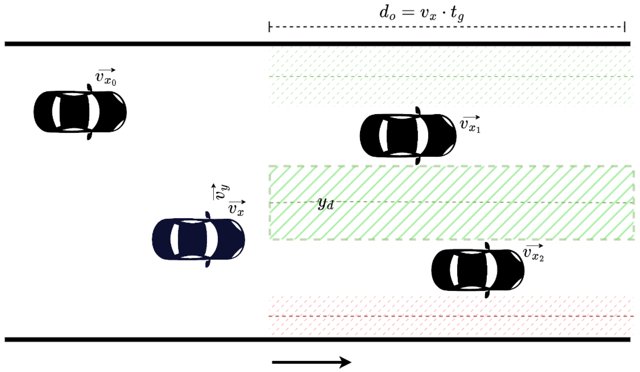
Figure 4.
Reward over time for different reward functions.
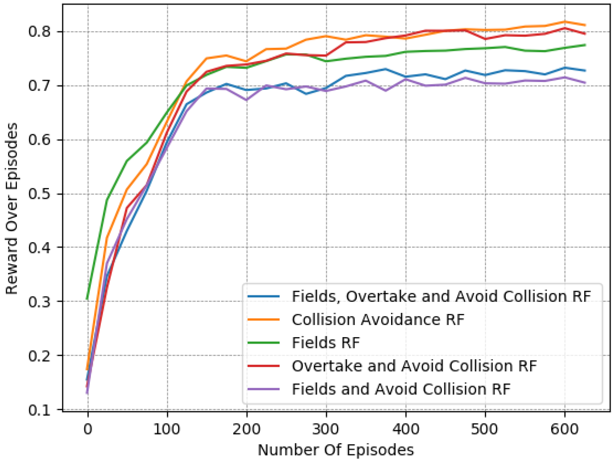
Figure 5.
Collisions over time for different reward functions.

Figure 6.
Speed deviation over time for different reward functions.
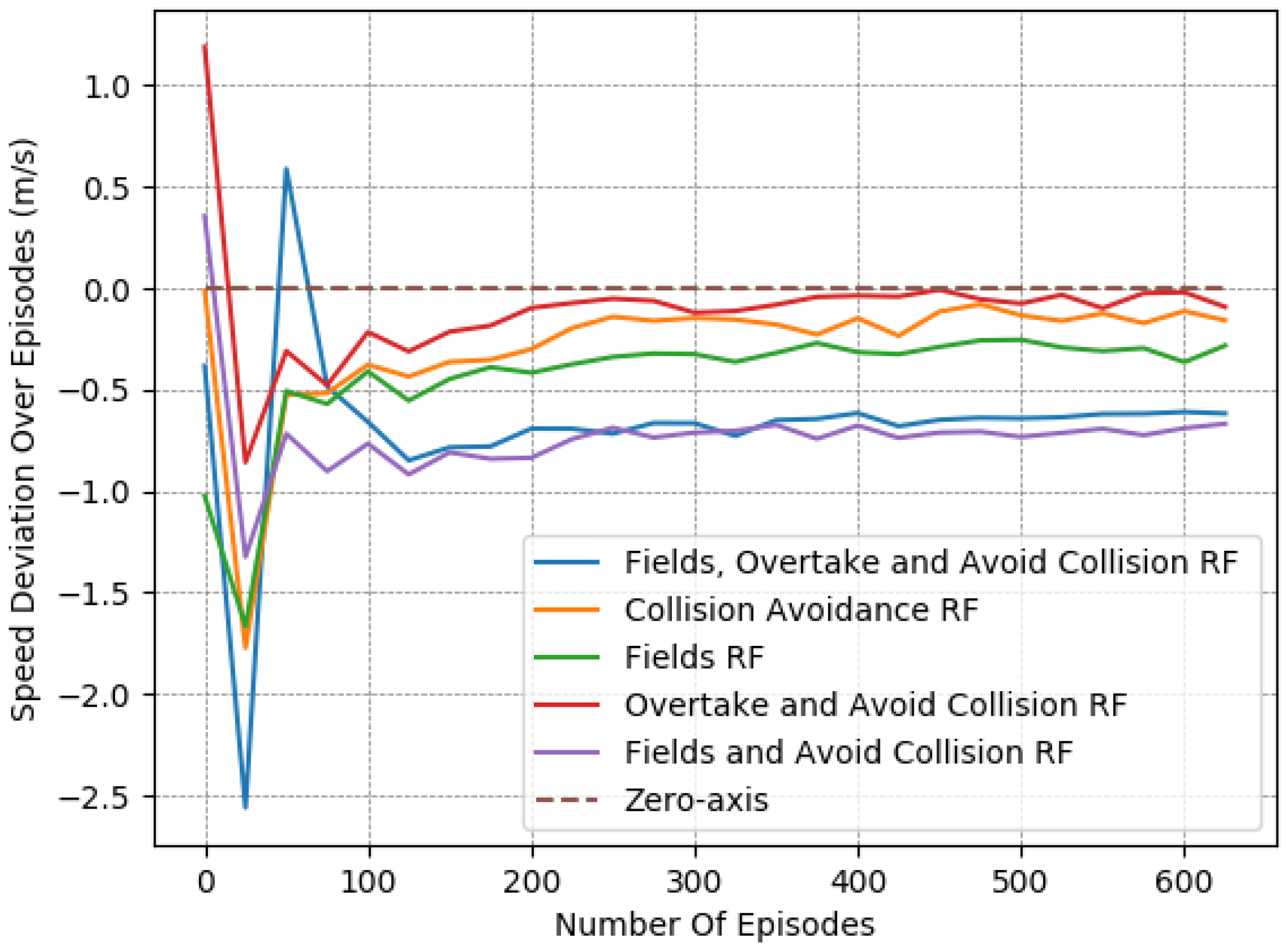
Figure 7.
Reward over time for different reward functions: evaluation of the zone selection reward component.
Figure 7.
Reward over time for different reward functions: evaluation of the zone selection reward component.

Figure 8.
Collisions over time for different reward functions: evaluation of the zone selection reward component.
Figure 8.
Collisions over time for different reward functions: evaluation of the zone selection reward component.

Figure 9.
Speed Deviation over time for different reward functions: evaluation of the zone selection reward component.
Figure 9.
Speed Deviation over time for different reward functions: evaluation of the zone selection reward component.
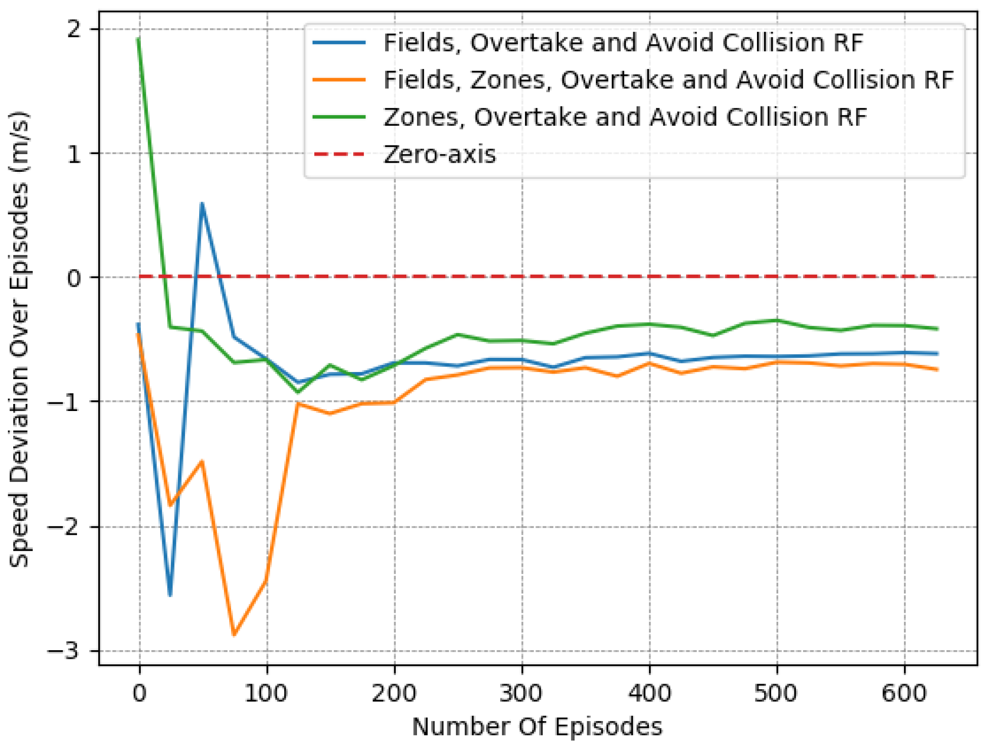
Figure 10.
Reward over time for the Fields, Overtake and Avoid Collision RF for different traffic densities.
Figure 10.
Reward over time for the Fields, Overtake and Avoid Collision RF for different traffic densities.

Figure 11.
Collisions over time for the Fields, Overtake and Avoid Collision RF for different traffic densities.
Figure 11.
Collisions over time for the Fields, Overtake and Avoid Collision RF for different traffic densities.
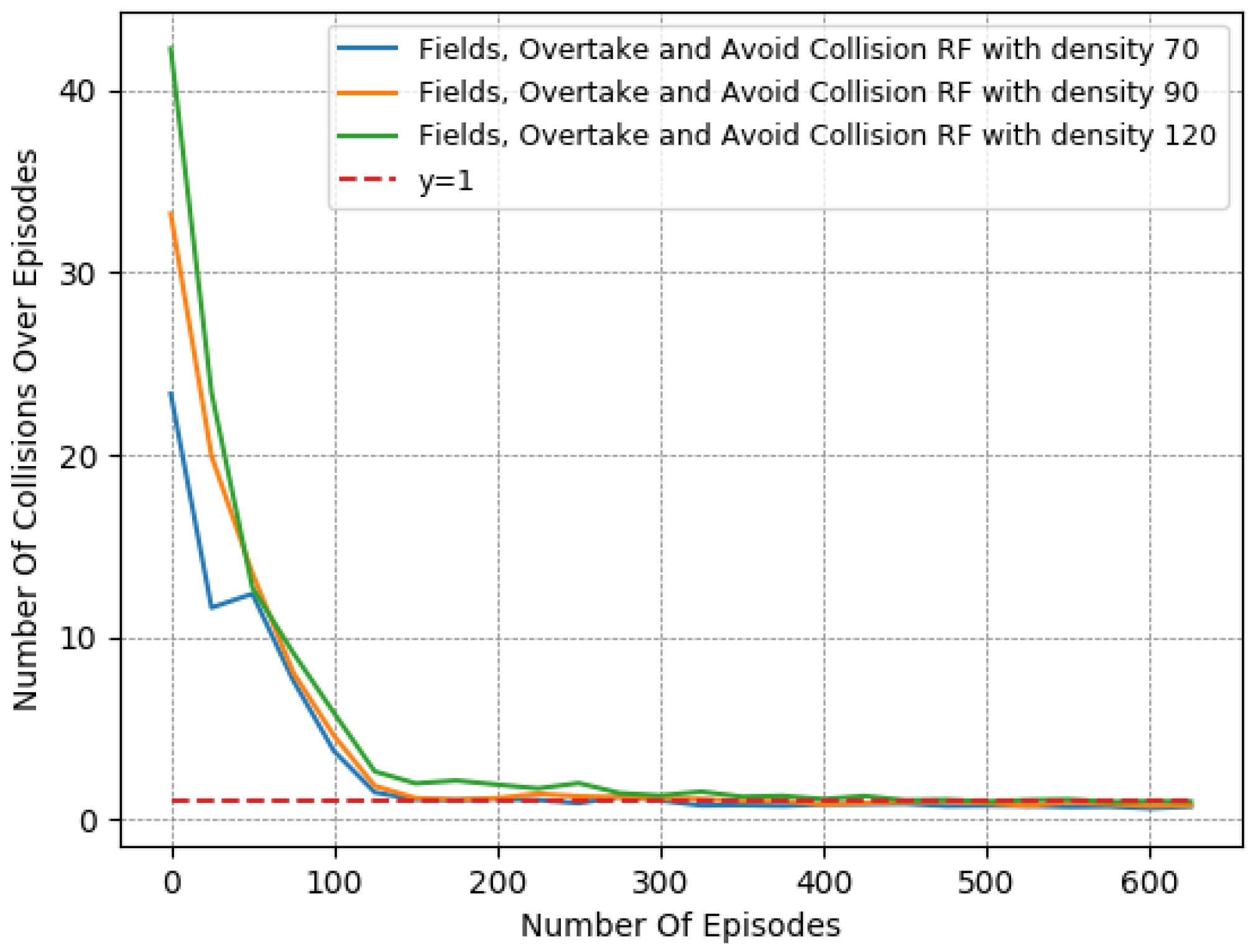
Figure 12.
Speed Deviation over time for the Fields, Overtake and Avoid Collision RF for different traffic densities.
Figure 12.
Speed Deviation over time for the Fields, Overtake and Avoid Collision RF for different traffic densities.
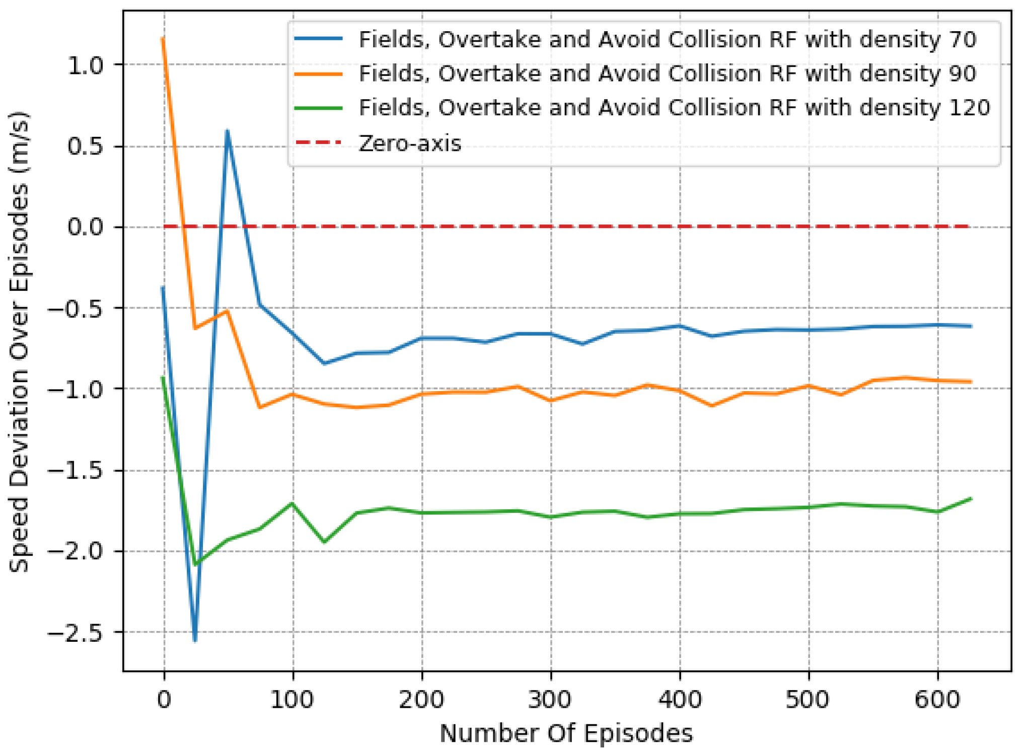
Figure 13.
Reward over time for the Fields, Zones, Overtake and Avoid Collision RF for different densities.
Figure 13.
Reward over time for the Fields, Zones, Overtake and Avoid Collision RF for different densities.
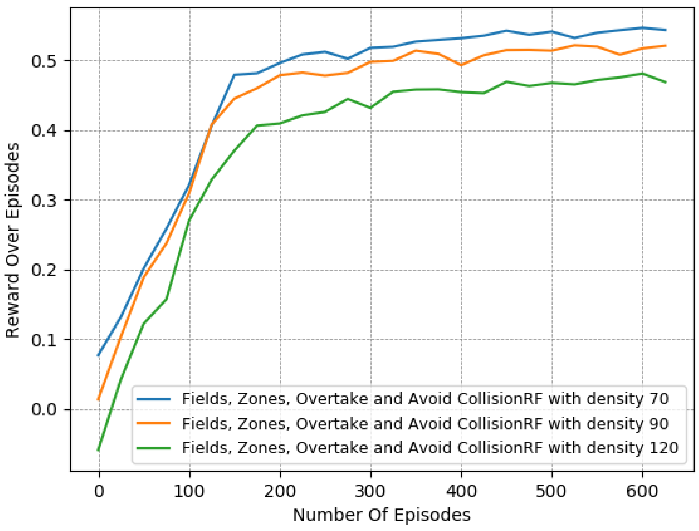
Figure 14.
Collisions over time for the Fields, Zones, Overtake and Avoid Collision RF for different densities.
Figure 14.
Collisions over time for the Fields, Zones, Overtake and Avoid Collision RF for different densities.
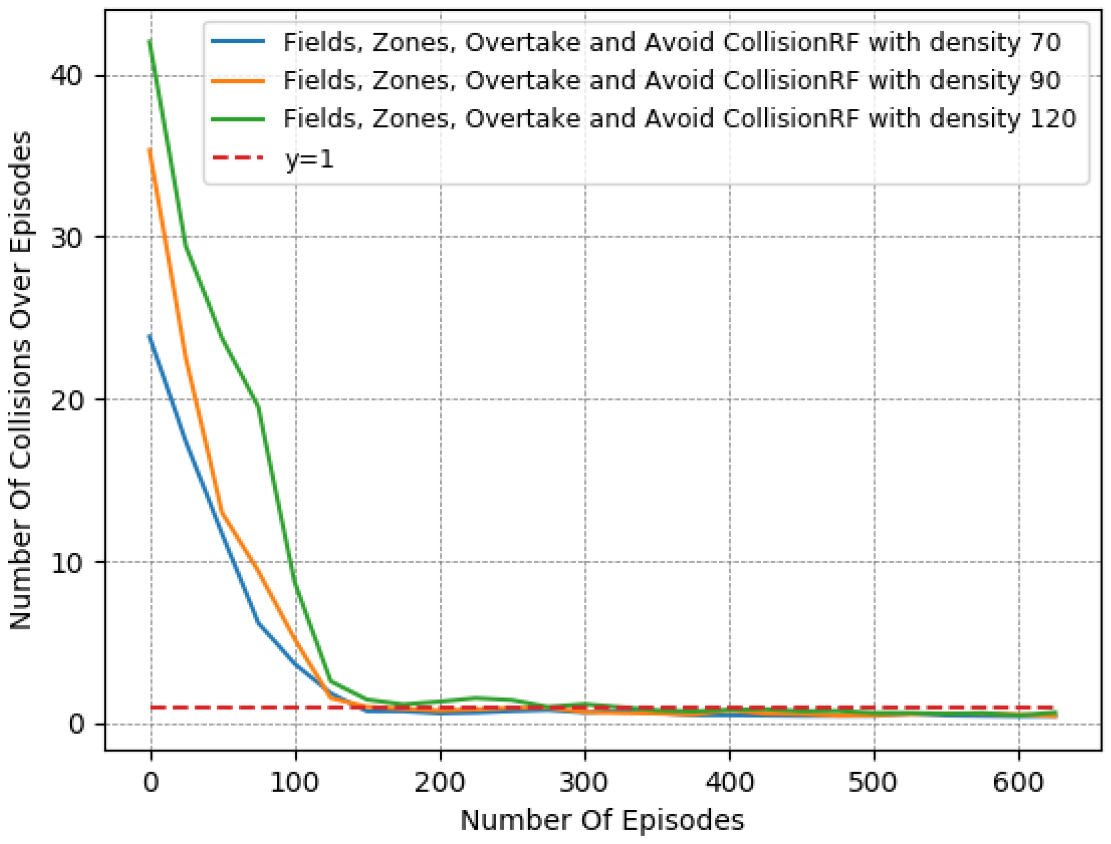
Figure 15.
Speed deviation over time for the Fields, Zones, Overtake and Avoid Collision RF for different densities.
Figure 15.
Speed deviation over time for the Fields, Zones, Overtake and Avoid Collision RF for different densities.
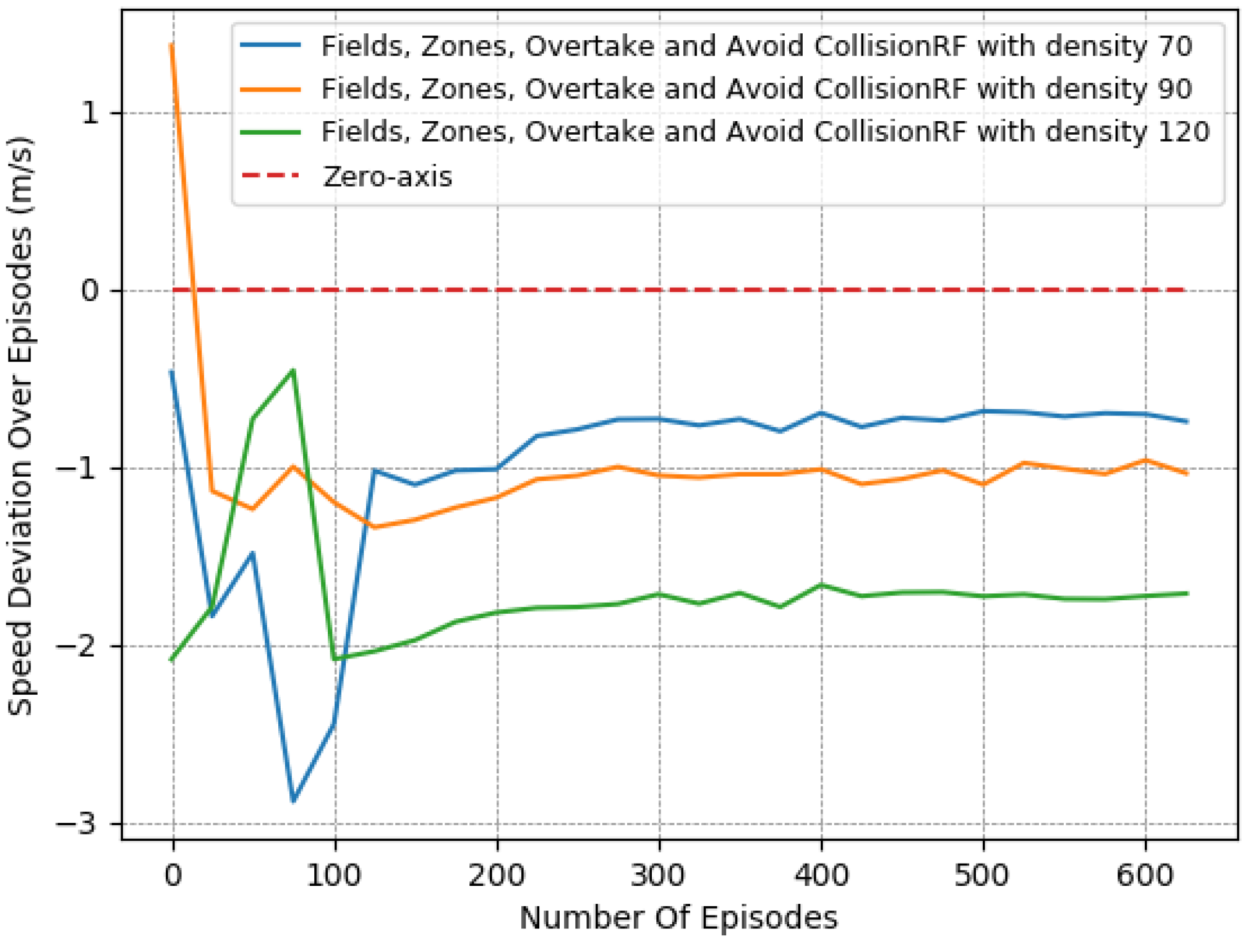
Figure 16.
Reward over time for the Fields, Zones, Overtake and Avoid Collision RF with different DRL algorithms.
Figure 16.
Reward over time for the Fields, Zones, Overtake and Avoid Collision RF with different DRL algorithms.

Figure 17.
Collisions over time for the Fields, Zones, Overtake and Avoid Collision RF with different DRL algorithms.
Figure 17.
Collisions over time for the Fields, Zones, Overtake and Avoid Collision RF with different DRL algorithms.
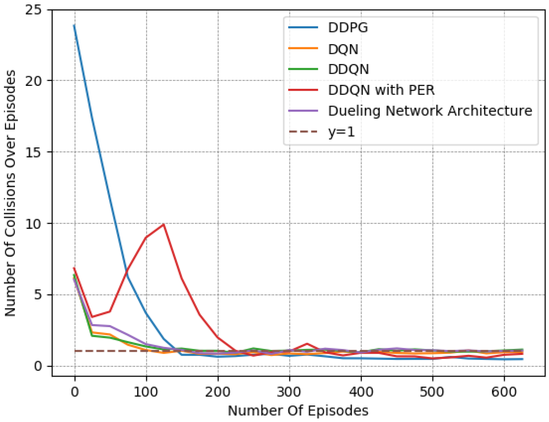
Figure 18.
Speed deviation over time for the “Fields, Zones, Overtake and Avoid Collision RF” with different DRL algorithms.
Figure 18.
Speed deviation over time for the “Fields, Zones, Overtake and Avoid Collision RF” with different DRL algorithms.


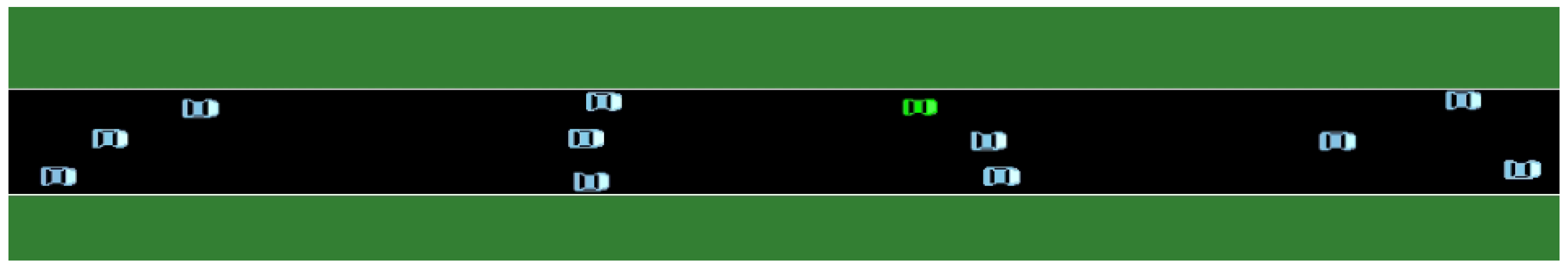
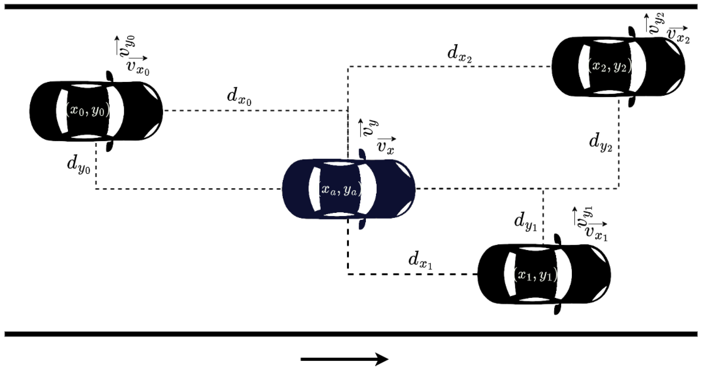
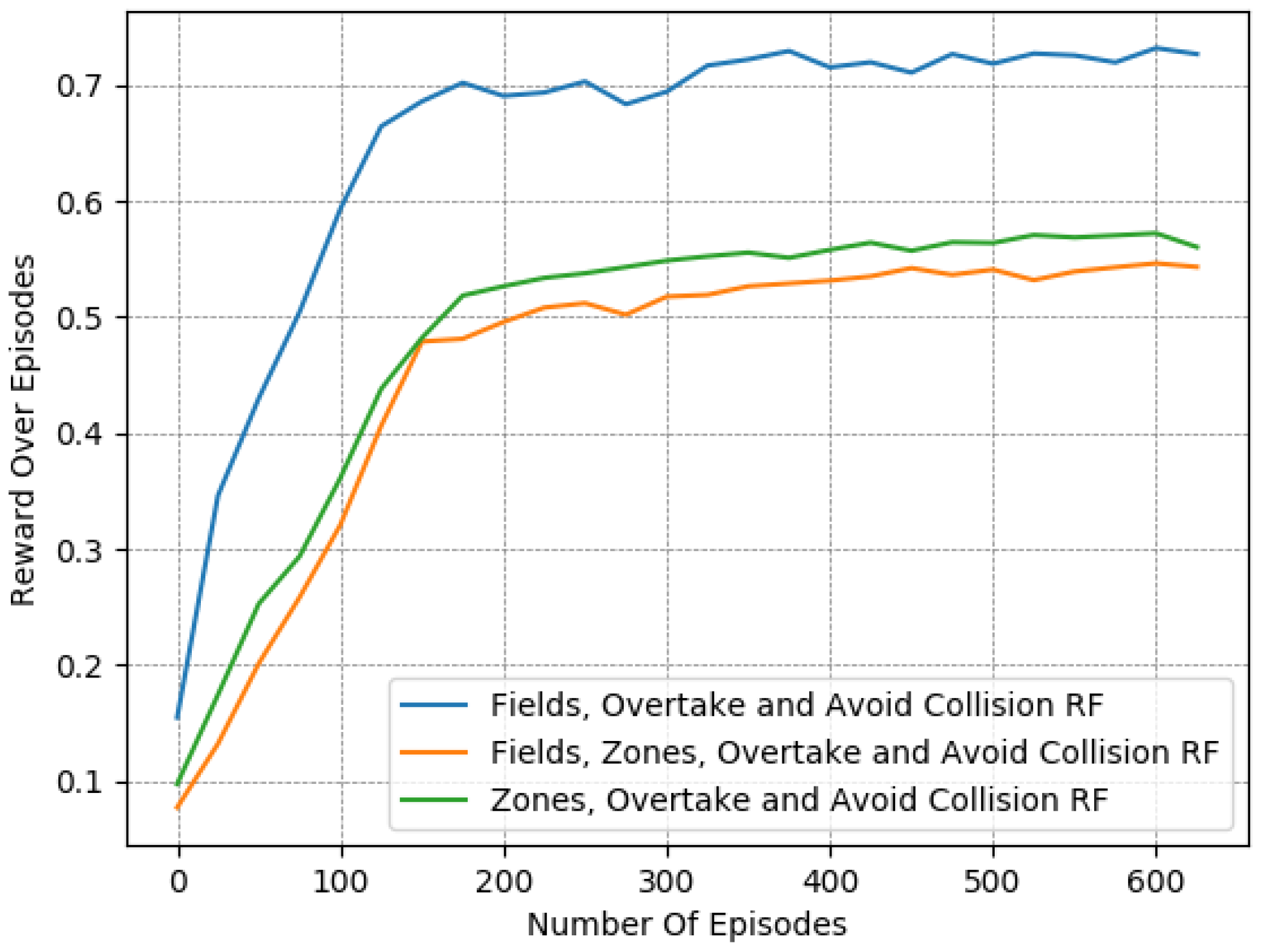
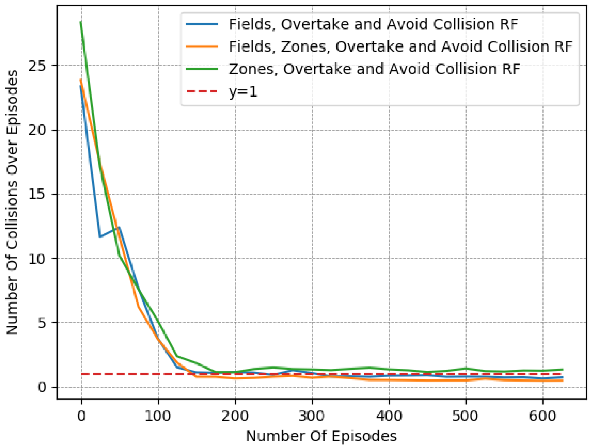
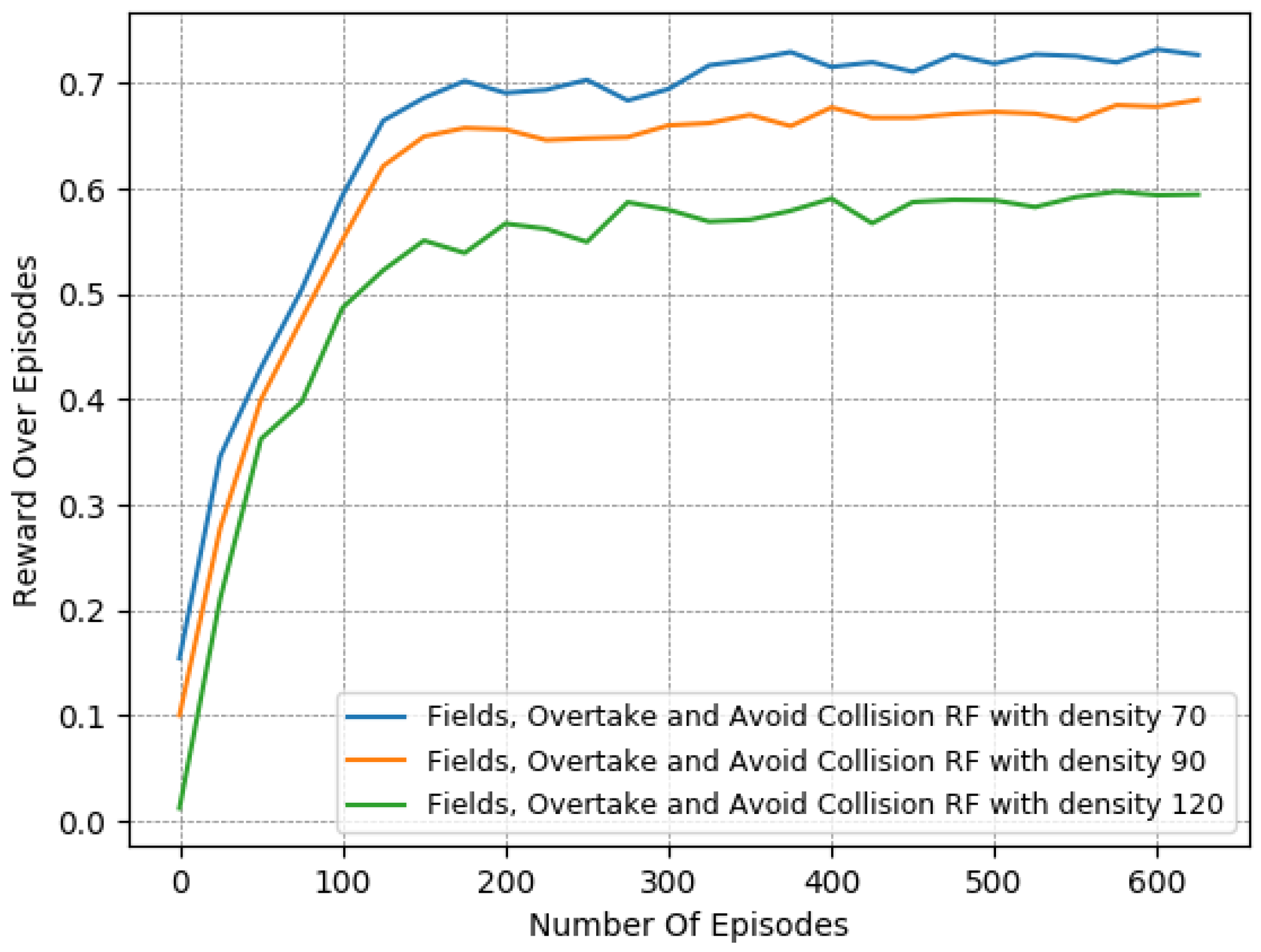
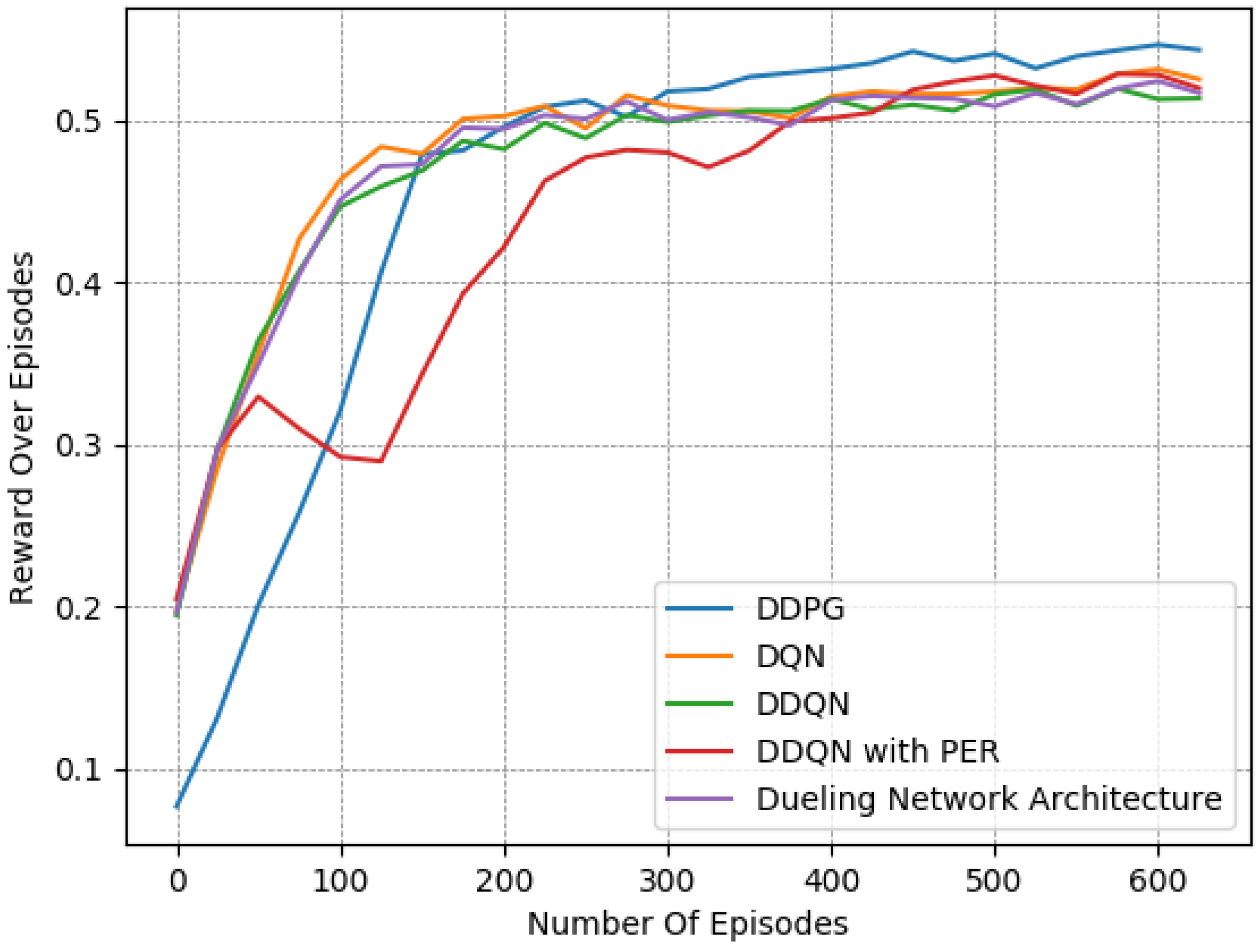
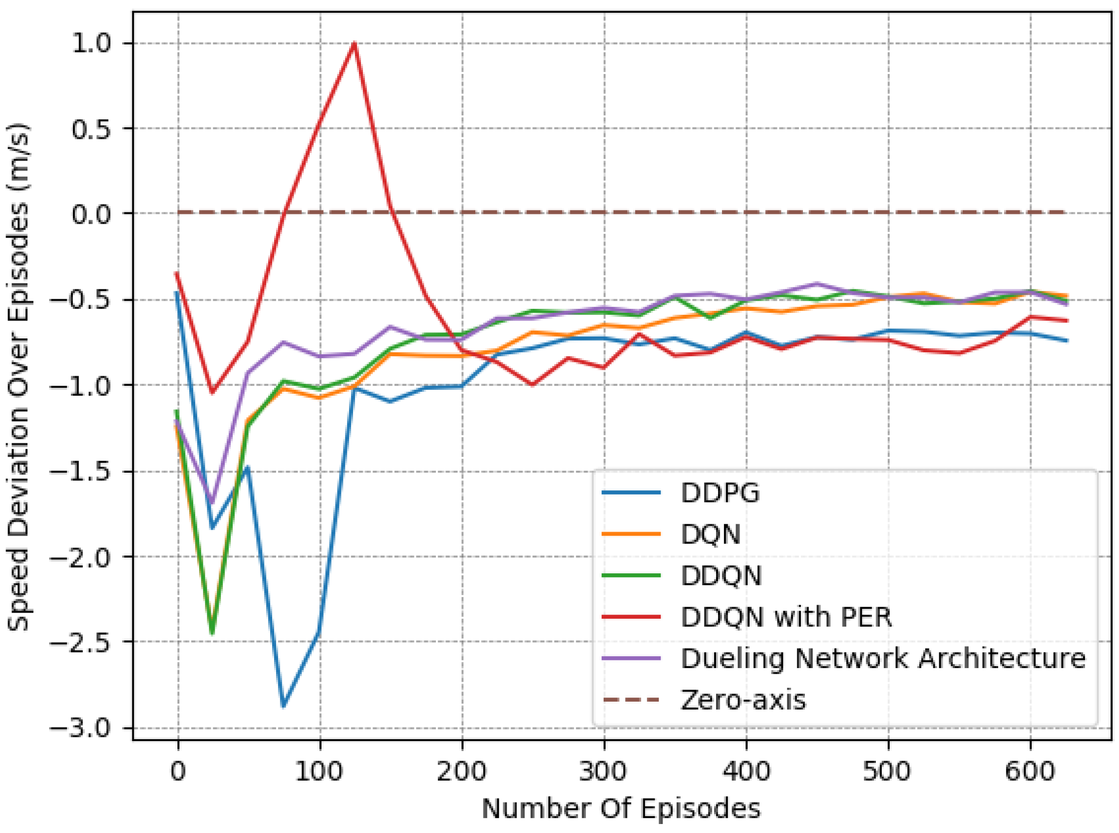
Table 1.
Hyper-parameters for RL algorithms.
| Parameter | Value | Parameter | Value |
|---|---|---|---|
| Learning rate used by Adam | 0.001 | Mini-Batch size | 64 |
| Discount factor (DQN) | 0.98 | Discount factor (DDPG) | 0.98 |
| Replay Memory size (DQN) | 50,000 | Replay Memory size (DDPG) | 100,000 |
| Soft update parameter (DDPG) | 0.001 | Number of episodes for training N | 625 |
Table 2.
Simulation parameters.
| Parameter | Value |
|---|---|
| Highway length | 500 m |
| Highway width | m |
| Vehicles’ length | m |
| Vehicles’ width | m |
| Types of vehicles | 2 |
| Num. of vehicles | 35 |
| Agent’s length | m |
| Agent’s width | m |
| Episode Time Length | 200 s |
| Time-Interval | s |
Table 3.
Parameter choices related to the MDP formulation.
| Parameter | Value |
|---|---|
| timegap | |
| agent’s desired speed | 20 m/s |
| other vehicles’ desired speed | 18 m/s to 22 m/s |
| num. of vehicles in state n | 5 |
| longitudinal observation distance d | 80 m |
| 1 | |
| (for RFs with lateral target) | |
| (for RFs without lateral target) | |
| 2 | |
Table 4.
All reward functions.
| Function Label | Equation | Component(s) Description |
|---|---|---|
| Collision Avoidance RF | Section 3.4.3 | |
| Overtake and Avoid Collision RF | Section 3.4.2 and Section 3.4.3 | |
| Fields RF | Section 3.4.4 | |
| Fields and Avoid Collision RF | Section 3.4.3 and Section 3.4.4 | |
| Fields, Overtake and Avoid Collision RF | Section 3.4.2–Section 3.4.4 | |
| Zones, Overtake and Avoid Collision RF | Section 3.4.2, Section 3.4.3 and Section 3.4.5 | |
| Fields, Zones, Overtake and Avoid Collision RF | Section 3.4.2–Section 3.4.5 |
Table 5.
Comparing the different reward functions.
| Reward Function | Collision Avoidance RF | Fields RF | Fields & Avoid Collision RF | Overtake & Avoid Collision RF | Fields, Overtake & Avoid Collision RF |
|---|---|---|---|---|---|
| Collisions | |||||
| Speed Dev. (m/s) |
Table 6.
Comparing the different reward functions: the effect of the “Zones” reward component.
| Reward Function | Fields, Zones, Overtake & Avoid Collision RF | Fields, Overtake & Avoid Collision RF | Zones, Overtake & Avoid Collision RF |
|---|---|---|---|
| Collisions | |||
| Speed Dev. (m/s) |
Table 7.
Evaluating the efficiency of the “Zones” reward component under different traffic densities.
Table 7.
Evaluating the efficiency of the “Zones” reward component under different traffic densities.
| Reward Function | Fields, Zones, Overtake & Avoid Collision RF | Fields, Overtake & Avoid Collision RF | ||||
|---|---|---|---|---|---|---|
| Density | 70 | 90 | 120 | 70 | 90 | 120 |
| Collisions | ||||||
| Speed Dev. (m/s) | ||||||
Table 8.
Comparing different DRL Algorithms with the “Fields, Zones, Overtake and Avoid Collision RF”.
Table 8.
Comparing different DRL Algorithms with the “Fields, Zones, Overtake and Avoid Collision RF”.
| DRL Algorithms | DDPG | DQN | DDQN | DNA | PER |
|---|---|---|---|---|---|
| Collisions | |||||
| Speed Dev. (m/s) |
Disclaimer/Publisher’s Note: The statements, opinions and data contained in all publications are solely those of the individual author(s) and contributor(s) and not of MDPI and/or the editor(s). MDPI and/or the editor(s) disclaim responsibility for any injury to people or property resulting from any ideas, methods, instructions or products referred to in the content. |
© 2023 by the authors. Licensee MDPI, Basel, Switzerland. This article is an open access article distributed under the terms and conditions of the Creative Commons Attribution (CC BY) license (https://creativecommons.org/licenses/by/4.0/).
Share and Cite
MDPI and ACS Style
Karalakou, A.; Troullinos, D.; Chalkiadakis, G.; Papageorgiou, M. Deep Reinforcement Learning Reward Function Design for Autonomous Driving in Lane-Free Traffic. Systems 2023, 11, 134. https://doi.org/10.3390/systems11030134
AMA Style
Karalakou A, Troullinos D, Chalkiadakis G, Papageorgiou M. Deep Reinforcement Learning Reward Function Design for Autonomous Driving in Lane-Free Traffic. Systems. 2023; 11(3):134. https://doi.org/10.3390/systems11030134
Chicago/Turabian StyleKaralakou, Athanasia, Dimitrios Troullinos, Georgios Chalkiadakis, and Markos Papageorgiou. 2023. "Deep Reinforcement Learning Reward Function Design for Autonomous Driving in Lane-Free Traffic" Systems 11, no. 3: 134. https://doi.org/10.3390/systems11030134
Note that from the first issue of 2016, this journal uses article numbers instead of page numbers. See further details here.