

The Hidden Side of Electro-Mobility: Modelling Agents’ Financial Statements and Their Interactions with a European Focus

1
European Commission, Joint Research Centre (JRC), 21027 Ispra, Italy
2
Department of Land Economy, University of Cambridge, Cambridge CB39EP, UK
*
Author to whom correspondence should be addressed.
Systems 2023, 11(3), 132; https://doi.org/10.3390/systems11030132
Submission received: 3 January 2023
/
Revised: 14 February 2023
/
Accepted: 16 February 2023
/
Published: 1 March 2023
(This article belongs to the Special Issue Advancements in the Practical Applications of Agents, Multi-Agent Systems and Simulating Complex Systems)
Abstract
:While much attention has been given, to date, to subsidies and taxes, the literature on the topic is yet to address less visible aspects of electro-mobility. These include the interactions among players, including money exchanges, and balance sheet issues. Analysing these is needed, as it helps identify additional mechanisms that may affect electro-mobility. This paper reports a modelling exercise that applies the system dynamics method, with its focus on stock and flow variables. The resulting simulation model captures the financial statements of several macro agents. The results show that the objective of the study is met: the model remains ‘stock-flow consistent’, meaning that assets and equity and liabilities balance out. By attaining this, the model serves as a coherent framework that makes the “hidden” side of electro-mobility visible, for the first time, based on current state-of-the-art, with the implication that it facilitates the analysis of potential financial factors that may either jeopardise or be conducive to faster road electrification. We conclude that the incorporation of the financial statements of key electro-mobility agents and their interlinkages in a simulation model is both a feasible and desired property for policy-relevant models.
1. Introduction
1.1. Background
The process of road transport electrification is complex, and the rate of growth of electric vehicle (EV) sales and stock is dependent on the actions of several major players. Focusing on electro-mobility in Europe, the Powertrain Technology Transition Market Agent Model (PTTMAM) represents four of these, grouped as market agents: Authorities, Infrastructure Providers, Vehicle Manufacturers and Users [1].
In this model, each agent makes a series of decisions which have an influence on one or more of the other agents (see Figure 1). For instance, users demand vehicles that are produced by manufacturers. While these decisions were modelled for aspects that tend to be rather visible (e.g., authorities set emission targets and infrastructure providers deploy recharging infrastructure), other aspects that are thought to be important, as well, tend to be less visible (remain “hidden”). These include, prominently, the financial position of each agent and the money inflows and outflows that determine it.
For example, Regulation (EU) 2019/631 stipulates that “the amounts of the excess emissions premium should be considered as revenue for the general budget of the Union” and the European Commission should consider the feasibility of allocating them to a fund “to support re-skilling, up-skilling and other skills training of workers in the automotive sector” [2] (p. 19). This is clearly a potential transfer of money from vehicle manufacturers to a public institution and, in turn, possibly to certain households, directly or indirectly via manufacturers.
Another example is the direct government support to original equipment manufacturers (OEMs). For instance, [4] reported EUR 295 million in government grants and subsidies in 2020, part of which was for alternative drive systems. [5] reported EUR 1 billion in government grants in the same year, though this OEM includes liquidity on favourable terms given by the European Central Bank (ECB) in that category.
A more indirect way of Member State (MS) support to vehicle manufacturers is as follows: the European Investment Bank (EIB) receives annual contributions from MSs; in turn, the EIB offers finance support to the automotive sector, as can be seen in Table 1. This table summarizes the evidence on EIB support to electro-mobility. Though the list is probably not exhaustive, it can yield a preliminary estimate of cumulative EIB finance support to the European automotive sector: ca. EUR 7 billion for research and development (R&D) actions and EV production support between 2010 and 2020.
1.2. Current State of the Research Field
The three examples mentioned in the previous section illustrate the importance of also taking into account the money flows among the key agents of the electro-mobility eco-system and, consequently, their financial positions. The extent to which this has been examined in the existing literature is considered in this section.
One of the most recent studies, which focuses on the electro-mobility sector and energy transition, applies hybrid econometric dynamic systems modelling based on Post-Keynesian economic theory, to address the energy transport transition in China, India, Japan, the United Kingdom and United States (US) [7]. Its objective is to demonstrate that the policy mix can support achieving tipping points where reinforcing learning and positive dynamics can support the transition relying on market driven forces alone. Similarly, [8] demands for economic modelling to investigate decarbonisation transitions at the global level, demanding financial incentives to the power and transport sector, still, with little ability to replicate the real structure of those sectors. In fact, those models apply policies while ignoring the “hidden” financial side of electro-mobility, leading to missing important leverage points that could support policy makers in addressing a faster energy and road transport transition.
Acknowledging that the literature on electro-mobility has expanded in the last few years, two previous review exercises reported by one of the authors are highlighted in [9], where system dynamics (SD) was identified as a prominent method to investigate the uptake of electric cars; in [10], a more in-depth review of a selection of SD models was performed. In comparison to earlier work (e.g., [11,12]), the current study extends previous modelling efforts by modelling balance sheets and assuring the stock-flow consistency (SFC) conditions, meaning an approach in which “the stocks and flows of both real and financial variables must be fully integrated, along with an explicit consideration of their dynamics” (Lavoie in [13]) (p. vii).
SFC modelling was prominently reported by [14]. The other author adopted the SFC modelling approach in previous work: [15] presented the Economic Risk, Resources and Environment (ERRE) model, which applies fossil fuels, agricultural and climate limits as boundaries to a growing economy. In ERRE, “a balance sheet approach is employed for every economic agent to assure stock-and-flowconsistency in the economy as a whole” (p. 184).
The need to account for financial aspects when modelling the low-carbon energy transition was highlighted by [16]. Turning to the more recent literature dealing with SFC and the low-carbon energy transition, the transmission channels of climate finance policies (the carbon tax and green supporting factor) were examined by [17], who also identified reinforcing feedback processes when modelling six sectors/agents. Using a similar structure for agents, [18] also investigated carbon taxation, with the finding that it leads to a higher level of green investments as a result of financing by commercial banks. According to [19], “a crucial gap remains, preventing macro model-based analysis of financing barriers and policy interventions that may accelerate the energy transition”.
We identify a persistent research gap: the balance sheets of the key electro-mobility players have, to the best of our knowledge, not been coherently modelled. We think that this is relevant because the financial division of an OEM tends to account for a sizeable proportion of the firm’s balance sheet and to interact with other players such as authorities, banks and households. To the authors’ knowledge, this aspect is not yet covered in the literature, and we take this opportunity to address this inconsistency, as it can be relevant to policy targeting an acceleration of the road transport transition. We adopted the methodology indicated in the next sub-section (which lists additional materials) to address this gap.
1.3. Objective, Focus and Structure
The present paper describes the approach followed to create a simulation model that represents the financial statements of those players. This was a prerequisite for the objective of the study: capturing the interactions (in terms of money flows) among key market agents, while ensuring that the model remains ‘stock-flow consistent’.
The present study covers the global vehicle market, with a focus on the European conditions. For the purpose of this work, the following changes were implemented to earlier versions of the PTTMAM model [1]: (i) the ‘infrastructure providers’ were renamed ‘suppliers’, and ‘users’ became ‘households’; (ii) the banking sector was modelled by including a conglomerate of private/commercial banks (selling also vehicle insurance), the European Central Bank (ECB) and the European Investment Bank (EIB); and (iii) the last two represent new sub-agents of the market agent group ‘authorities’, which now includes government as a separate sub-agent.
2. Materials and Methods
2.1. Methodology
The methodology was implemented following a series of steps:
- The financial statements of OEMs (i.e., vehicle manufacturers) were collected from their annual reports and data from the U.S. Securities and Exchange Commission filings. As for any other firm, the three main financial statements of OEMs are: a balance sheet, an income statement and a cash flow statement. Each of them facilitates the analysis of, respectively, solvency, profitability and liquidity. There are two broad economic and financial decisions firms need to make: investment (maximise profitability) and financing (minimise capital costs). Whereas the former is visible in the assets side of a balance sheet, the latter can be reflected in the equity and liabilities section [20]. Instead of profit maximising, “some companies may respond to daunting balance-sheet damage by minimizing debt” [21] (p. xii). This is a sufficient reason for us to model debt explicitly.
- Two balance sheet items (PPE and inventories) require an explanation, as their values can be affected by alternative assumptions. For each of them, we first read what the accounting rules are; we then check what has been assumed in previous SD work and identify what most OEMs adopt in practice.
- The information collected from the previous steps was implemented in the simulation software environment ‘Vensim’. A reference that was used for the preliminary version is [25].
- The variables for the initialisation of the model were created and initial values (see Table 2; money values are expressed in nominal terms) were assigned to those, so that the behaviour resulting from the structure represented in the model (step 4) could be simulated for the period 2005–2030. This was based on numerical integration using Euler, with a time step of 0.25 year (see, e.g., [26]).
- The structure was refined until there were, a priori, no financial leakages in the modelled system.
- The monetary structure was linked with the physical structure (e.g., revenues from selling vehicles) from which a series of key performance indicators (KPIs) could be computed.
The outlined methodological approach relies on the following steps. The initial part is statistical and includes the sourcing of relevant initial values. Furthermore, the ‘double-entry bookkeeping’ rule from the field of accounting [27] is imposed. The implementation in the software requires the use of stock and flow variables, which are connected in stock and flow structures (see, e.g., [28]). As stated by [29], stocks and flows are not independent, as the former result from the latter, and flows are also influenced by stocks. Thus, a two-way relationship between these variables may be posited. At the core of this methodology is the reliance on the SD method, which is well-suited for searching for the economy’s feedback structure [30]. Ref.[13] concluded that SD is a robust method to assure SFC conditions are met.
2.2. Model
2.2.1. Overview
Figure 2 provides an overview of the developed model. As can be seen, the private and public sectors interact in several ways, as transactions among agents take place in our simulated environment. Initial stock values do not reflect data collection but are assumed for the purpose of demonstrating the modelling framework. On model testing, see Appendix A. The simulation model is freely available at the webpage shown in the Supplementary Materials.
Focusing on the interlinkages among ‘Banks and insurance’, ‘Households’ (HHs) and ‘OEMs’, Figure 3 shows four balancing (B) feedback loops and five reinforcing (R) ones. They describe the debt dependency process, the amplifying nature of borrowing to acquire liquidity and pay interest, as well as the counteracting effects of debt adjustment and repayment. This is highlighted in Figure 3 as the “hidden” side of electro-mobility and forms a core component of this paper. At the top of the figure, a key aspect of electro-mobility is made visible, as EVs are still priced higher than conventional vehicles and thus require substantial upfront payments from HHs. While this causal loop diagram informed the modelling building process, it remains a simplification, as the link between borrowing from the OEM and vehicle purchase is mediated in the simulation model by the stock ‘wealth HH debtor’. Moreover, the figure provides a stylised overview, with ‘Banks and insurance’ (green area) overlapping the other two agents.
2.2.2. Authorities
Authorities represent the public sector, which, as indicated above, consists of governments and selected EU institutions. Table 2 lists the initial values of these sub-agents.

Table 2.
Initial values of the authorities’ balance sheets [EUR].
| Sub-Agent | Assets | Liabilities & Equity |
|---|---|---|
| ECB | 6 × 10¹² | 6 × 10¹² |
| EIB | 2.8 × 10¹¹ | 2.8 × 10¹¹ |
| Government | 1011 | 1011 |
Source: own assumptions.
The government is defined as a single entity (i.e., without disaggregation by country) in the present version of the model to facilitate the analysis. The liabilities side of the balance sheet consists of bank debt (in this hypothetical case, to the central bank). The simulated government budget is affected by three revenue items (corporate tax, energy tax, value-added tax (VAT)) and four expenditures:
- Public infrastructure expenditures, calculated as follows: the historical and projected electric vehicle supply equipment (EVSE) values for the world, disaggregated into slow- and fast-charging points, provided by [31], are incorporated into the model. The project values reflect the STEPS scenario and are interpolated linearly as needed. The resulting estimates are used to compute annual deployment under the assumption that EVSE is long-lived. Next, the cost of the EVSE is as follows: EUR 9000/point for slow and EUR 100,000/point for fast. We work under the premise that the government provides the required funding for the deployment of such publicly accessible infrastructure.
- Public R&D expenditures: this variable is included and linked to OEMs to facilitate the analysis of government grants to the automotive industry. However, in the current version of the model, it takes a value of zero.
- Public transport procurement: all buses are purchased by this agent.
- Purchase subsidies: estimates of government purchase subsidies for the period 2016–2021 were collected from [32], with a linear decline to zero in 2025 assumed.
Concerning revenues, it is assumed that taxes represent half of the fuel price. The simulated VAT rate is 20%.
EU institutions are modelled in a very basic fashion (see Figure 4 for the example of the ECB). As can be seen in this figure, ECB assets consist of loans (to commercial banks and governments) and cash. The grey variables within the <> signs are known in the SD literature as ‘shadow variables’ and represent variables that are defined in another part of the model. For instance, ‘debt to central bank’ is defined as a stock variable in the ‘Banks and insurance’ agent.
The interest policy rate is fixed at 3%. Concerning the EIB, a favourable rate of 4% is available to OEMs. To make the model operational, it is assumed that the potential revenues from missing vehicle emissions targets are available to the Union’s budget via the EIB.
2.2.3. Banks and Insurance Firms
This agent represents a conglomerate of commercial/private banks that engage also in insurance services. The insurance premium is assumed to be EUR 500 vehicle/year. The annual percentage rate (APR) is simulated with a constant value of 5%. Table 3 shows the initial values of the balance sheet items modelled for this agent.
2.2.4. Households
HHs are divided into two sub-agents: creditor and debtor. The key difference is that the latter holds debt (to banks and OEMs). Another difference is that, while the debtor HH receives the labour wages from vehicle manufacturing, the dividends are accrued to the creditor HH. The wealth of this sub-agent is stored as deposits in the private banking system. As for the other agents, Table 4 shows the key initial values. Most of the cars (with the exception of those registered by OEMs for leasing/rental purposes) are purchased by these two sub-agents, with an equal split in share. The historical and projected global battery electric vehicle (BEV) stock, disaggregated into vehicle type, provided by [31], was fed into the model.
2.2.5. Suppliers
This agent represents a conglomerate of raw material, battery, energy, infrastructure and vehicle maintenance providers. The corresponding items related to these become sources of annual revenue for this agent. Its assets are initially valued at EUR 1e+12. Suppliers deploy the publicly accessible EVSE commissioned by governments, with depreciation influenced by an average lifetime of 20 years for this asset. Moreover, the Suppliers are the agent purchasing freight vehicles (vans and trucks).
Three types of fuels are supplied by this agent: petrol and diesel for ICEV (the former for cars, and the latter for the rest) and electricity for BEVs.
The markup over cost set by the Suppliers is 20% (a reasonable assumption; see, e.g., [33]), both for raw materials and batteries. The maintenance cost is EUR 300 vehicle/year (for a range by manufacturer see [34]). See the time-variant values used for the exchange rate and the battery and fuel prices in the Supplementary Materials.
2.2.6. Vehicle Manufacturers
By far, the most elaborate agent in our model is the OEM. This agent includes a hypothetical domestic and foreign OEM, each one holding a market share of 50%. Table 5 shows the initial values assigned to each of the two OEM conglomerates, comparing total assets with the sum of liabilities and equity (L&E). Each of them is duplicated, for OEMs are subscripted in our model into Automotive and a Financial Divisions, in line with the information gathered from their annual reports. As can be seen, simplifications of several items were made, and their weight greatly differs by division. For the rest of the agents, these statements are more simple. As expected, OEM debt becomes an asset for commercial banks (recall Table 3). Conversely, HH debt tied to vehicle purchases is captured in financial services receivables (current and noncurrent), which are an asset to the OEM. The evidence on car finance is provided by, for example, [35].
As hinted above, the first balance sheet item requiring an explanation is PPE, which is affected by depreciation. According to the Generally Accepted Accounting Principles (GAAP) and International Financial Reporting Standards (IFRS), acceptable depreciation methods include straight-line, accelerated and units-of-production methods [22]. Straight-line depreciation was adopted in the SD accounting model by [36]. While there are differences across individual OEM and years, our analysis of OEM financial information leads us to conclude that the straight-line method was the main one adopted over the past decade in this industry. We thus implement this method in our model, following [36]. Assuming that annual vehicle sales remain constant (see Section 2.2.4), plant acquisition is kept constant at EUR 10 billion annually. Investment in vehicles to generate lease revenues amount to EUR 55 billion per year. Annual depreciation and amortisation expenses equal EUR 64.5 billion.
The second item is inventories, whose valuation differs by method. While GAAP accepts the weighted-average cost, first-in, first-out (FIFO) and last-in, first-out (LIFO) methods, IFRS prohibits the use of LIFO [22]. Implementing the average cost method in his model, [36] regards it as the only reasonable one to account for inventories in an SD model, acknowledging that this method is not used by most firms. In our model, we compute physical inventories and their values for four types of vehicles: cars, vans, trucks and buses. These are kept constant over the simulation period.
Table 6 shows additional assumptions made for OEMs. Furthermore, it is assumed that OEMs self-register cars for leasing/rental purposes, with the fleet owned by the Financial Division increasing from almost 14 million cars to almost 27.5 million in 2030. An annual transfer amounting to EUR 30 billion from the Automotive to the Financial Division is simulated.
Focusing on the different types of vehicles modelled, Table 7 lists key assumptions. Each vehicle type is also disaggregated into an internal combustion engine vehicle (ICEV) and a BEV. While the labour costs are assumed to be the same for the two technologies, besides the battery the material costs differ. The table also shows two assumptions that are important for the calculation of the fleet’s energy demand, which is needed to compute expenditures on energy products.
3. Results
3.1. Evolution of the Vehicle Fleet
A selection of the model results for the various agents is presented below. All the figures refer to a simulation run named ‘Current’. Figure 5 shows the evolution of the vehicle stock, disaggregated by the type of vehicle and technology. The BEVs exhibit growth at the expense of the ICEVs, though the latter still dominates at the global level in 2030. This is the type of output most models consider, but what are the potential economic and financial implications for the agents involved in this system? The “hidden” side of electro-mobility becomes visible, based on our simulation framework, in the next figures.
3.2. Balance Sheets
As vehicle sales require vehicle production and demand, and both are partly financed with debt, it becomes useful to consider the structure of the liabilities and how it is connected to other agents’ assets. For instance, HH debt to OEMs for the purpose of purchasing vehicles constitutes an asset for the latter, and the debt of the two agents to private banks represents a fraction of the total assets owned by these. EIB loans to OEMs to facilitate cleaner vehicle production also feature in the assets side of the EIB balance sheet. The Central Bank’s assets may also be formed of loans to governments and private banks. This means that the overall behaviour of the system is the result of the interaction between the macro agents (recall Figure 2).
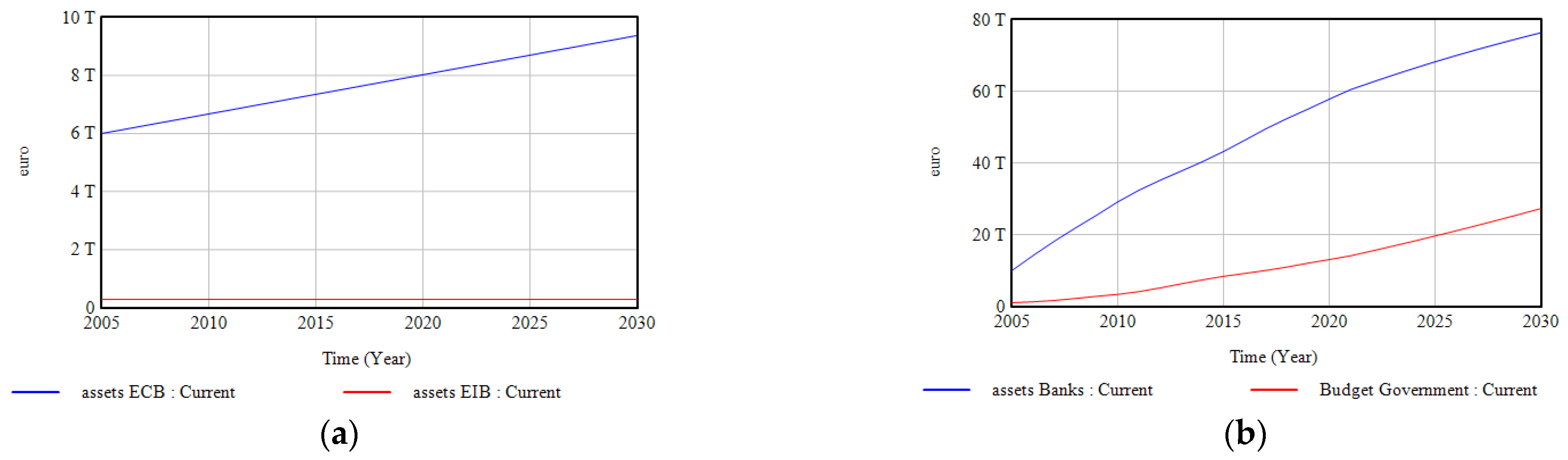
Figure 6 shows the simulated evolution of assets (and thus L&E) for two agents. While the chart on the left shows the output of the two public banks, the behaviour of private banks and the government can be seen in the chart on the right. The balance sheet expands in all cases, though very slowly in the case of the EIB.
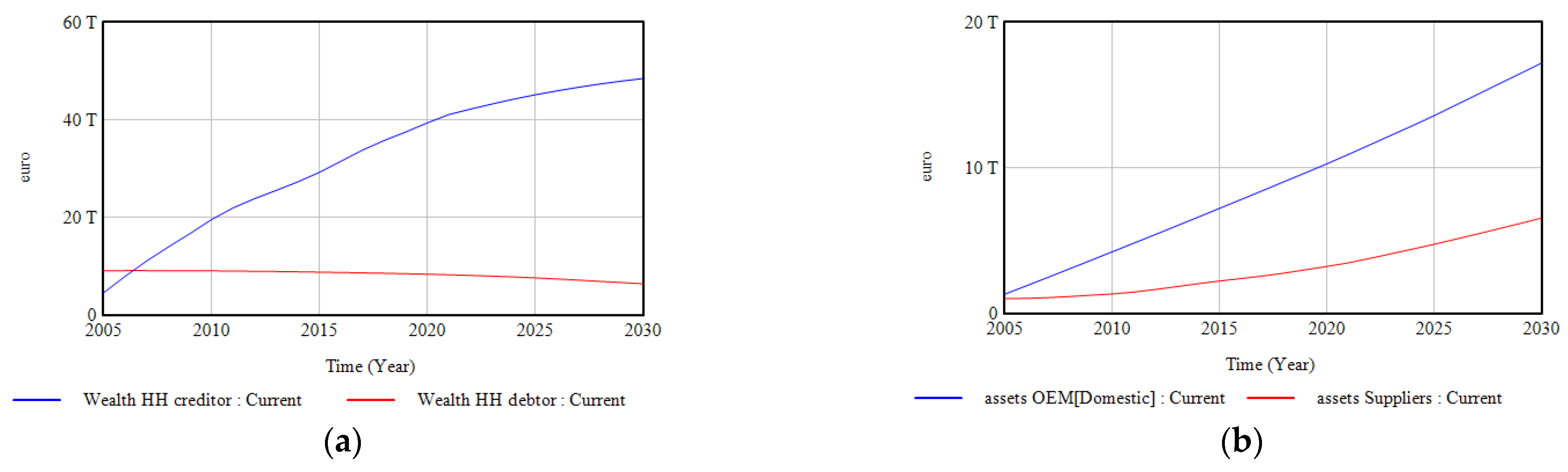
Similarly, Figure 7 shows the simulated evolution of the balance sheet for the rest of the private sector. As can be seen on the left chart, the wealth of the creditor HH quickly overtakes that of the debtor, which declines slowly towards the end of the simulation. The chart on the right shows the growing assets of the suppliers and vehicle manufacturers, which diverge from a similar base in 2005 until the assets of each OEM doubles in size those of the suppliers in 2030.
What drives the changes in balance sheets are flow variables. For instance, the annual interest paid by HH debtors to OEMs amounts to slightly more than EUR 35 billion (or EUR 1083 per vehicle sold). This is an example of additional results generated by the model which, for reasons of space, cannot be reported here (see the Supplementary Materials instead). Variable OEM profits (growing, in particular, in the Financial Division) not only accumulate into retained earnings but also boosts dividends, which increase the wealth of creditor HHs. The simulated behaviour of ‘net savings HH creditor’ is always positive but exhibits a downwards trend, with swings between 2008 and 2020. This variable affects the stock and flow structure related to bank deposits, which leads to bank deposits growing until 2030 at a slower rate.
Moreover, the flow variables tend to be influenced by business operations and items from the income statement. Besides the physical ones (e.g., sales in Section 3.1), money items such as ‘dividends paid’ play a role. This flow is determined by the dividend distribution ratio (Table 6) and the net income, which is, in turn, used to compute a key performance indicator (KPI), examined next.
3.3. Key Performance Indicators
The computation of KPIs facilitates so-called ratio analysis. Our analysis of OEM reports confirmed our expectation that KPIs are important to OEM decision-makers. While the purpose was not to create a model to improve the behaviour of the automotive industry from an OEM perspective, it is useful to report the four standard profitability KPIs and an operating return KPI: the return on equity (ROE). This is done in Table 8, which also lists, for comparability, typical values found in the literature. Each KPI was computed following [22]. The ROE is reported for the Financial Division, as is common in the sector, while the profitability ratios correspond to the Automotive Division. In our simulation, the ROE peaks with a value of almost 16% in 2007, the year in which the global financial crisis began. As other sources of income were not assumed, our earnings before interest and taxes (EBIT) are the same as the operating income, and thus the two ratios show the same values.
By adding KPIs, the decisions of OEMs may be more sensibly modelled. In a way, this helps integrate the physical and financial sides of the OEM business. Our simulated KPI values are within the ranges derived from the data. The fact that the ones for profitability are closer to the 75% quartile while, in reality, some OEMs struggle to exhibit strong KPI performance is likely to be due to our assumption that the global vehicle market is served by a duopoly. In practice, OEMs set target margins that may be attained or not. Moreover, those targets may vary by year, depending on the management’s perception of business and international conditions. For instance, [37] reports how distant their adjusted target range for the automotive EBIT margin was from their target range.
4. Discussion
The automotive industry is undergoing radical transformation. The challenges faced by the sector in response to the presence of climate urgencies were clearly articulated by [38]. The importance of analysing the balance sheet to gauge the success of the business was highlighted by [39]. There seems to be an emerging need, relatively neglected in the existing literature, for researchers and policy-makers to put the potential emission penalties into the broader context of OEMs’ financial position and to understand the channels through which money flows (e.g., to promote R&D in cleaner vehicles, to finance zero-emission powertrain sales) among market agents. The present paper represents one step forward towards addressing this need.
The paper describes a simulation model to facilitate such analyses. We came across the work by [36] after we built our accounting framework but incorporated some of the features suggested by the author (recall Section 2.2.6).
Model testing was proposed as a means to demonstrate the standard behaviour of the model without aiming to explore either large sensitivities and uncertainties in every single parameter, or behaviour reproducibility tests based on historical data. This is in line with the purpose of this paper, which was to highlight the existence of the “hidden” side of the automotive sector, with OEMs ultimately behaving as financial institutions providing loans and receiving interest payments from their clients. Standard tests in line with the SD literature were performed, such as integration error tests, and unit consistency as indicated in Appendix A.
One way of exploring uncertainty is to compute alternative vehicle sales growth rates. This would then alter OEM manufacturing capacity needs and, in turn, investment in PPE. According to [40], retained earnings finance most EU firm investments. This would have implications for Figure 7b, which would also change if greater bargaining power were accorded to Suppliers. By making the model available, we facilitate this type of analysis being carried out by the interested reader.
The model assures full consistency in keeping the economic and financial flows within the system. By interlinking the money flows among the agents, it is possible to trace how money circulates within the automotive sectors. In particular, this allows analysts to keep track of cumulative public and private expenditures, such as purchase subsidies and R&D expenditures, respectively.
The simulated vehicle fleet suggests that petrol and diesel-powered vehicle remain the dominant technology until 2030, which would have environmentally damaging consequences unless other actions are taken. This picture could be altered if government grants and subsidies in support of innovations that lower emissions were simulated (recall Section 2.2.2). The important role public banks have to play in the transition to net zero has most recently been highlighted by [41].
Turning to our balance sheet results, by distinguishing between debtor and creditor HHs, we are in a position to start investigating distributional issues (e.g., automotive dividends and wages). However, a key limitation of our work is that it depicts HHs and governments as aggregated entities. A more realistic representation would disaggregate them by country. We felt that such level of detail would obscure the present exercise and be, thus, counterproductive.
While debt was modelled and securities were included explicitly in the OEMs’ assets, the capital and financial markets were portrayed in a simple manner. No explicit reference was made to, for example, money markets, commercial papers or corporate bonds (see, e.g., [42]) or risk management (see OEMs’ reports). No leverage, liquidity and valuation ratios were calculated, as outside of the main purpose of our model, but these could be easily added in the system, based on the version proposed.
The focus was on interrelated patterns rather than realistic numerical outcomes. While these may not correspond to actual data, setting the initial asset values to EUR 1 trillion for governments and suppliers (close to the estimated value for OEMs) was not completely undeliberate, for it facilitated the comparison of behaviours unfolding from a similar base. The sum of all the assets in our model amount to EUR 150.6 trillion in 2020. To put this into context, [43] estimated that the world economy had USD 1540 trillion in assets in the same year, of which one-third corresponded to real assets. Further data refinements may be made in the future: for the ECB, using [44], for the EIB, relying on [45], and for governments, using the Public Sector Balance Sheet (PSBS) The database is available at [46].
We conclude that the incorporation of the financial statements of key electro-mobility agents and their interlinkages in a simulation model is both feasible and a desired property for more realistic and policy relevant models. After all, the process of electrification does not follow solely from policy prescriptions but is the result of the way the key players digest relevant information, including financial. Taking these aspects into account in a modelling framework leads to an explicit generic representation of the banking sector. The downside of this is that the model becomes larger and understanding it more demanding. Still, we conclude that the benefits of this approach outweigh its costs, as it brings a perspective other modelling tools neglect.
Though we modelled the global vehicle market, we opted for defining authorities in European terms. For this reason, references to the ECB, EIB and the EU were made. This was done to emphasise the emission penalties that are relevant in the EU context (as this was one of the points made in the Introduction). However, such agents can be defined in more general terms (e.g., central bank instead of the ECB or public investment bank instead of the EIB), and the structure can, in principle, be applied to other markets. As a matter of fact, no excess emissions leading to penalties were simulated. To compute this in a robust manner, a representation of the existing regulations is needed. This is indeed the key connection point between the model proposed here and PTTMAM, which models HHs (‘Users’) and ‘Authorities’ with disaggregation by country. Such model integration will be pursued in future work. While there may be physical constraints that limit the speed of EV uptake (e.g., battery supply bottlenecks), the resulting model upgrade would enable the analysis of potential financial aspects.
The SFC framework proposed here makes the “hidden” side of electro-mobility visible, with the implication that it facilitates the analysis of potential financial constraints that might also jeopardise faster road travel electrification. Conversely, it may help identify the levers in the system for more effective financial support.
Supplementary Materials
Supporting information can be downloaded at http://data.europa.eu/89h/2086b2cb-3f20-4241-b8f8-00fa99969f86.
Author Contributions
Conceptualization, J.J.G.V.; methodology, J.J.G.V. and R.P.; software, J.J.G.V. and R.P.; validation, J.J.G.V. and R.P.; formal analysis, J.J.G.V. and R.P.; data curation, J.J.G.V.; writing—original draft preparation, J.J.G.V.; writing—review and editing, R.P.; visualization, J.J.G.V. and R.P.; project administration, J.J.G.V. All authors have read and agreed to the published version of the manuscript.
Funding
This research received no external funding.
Institutional Review Board Statement
Not applicable.
Informed Consent Statement
Not applicable.
Data Availability Statement
The data is included in the Supplementary Materials.
Acknowledgments
We are very grateful to two anonymous reviewers and an internal reviewer for their comments. We are also grateful to three anonymous reviewers from the Transportation Research Board’s Standing Committee on Economics and Finance for their helpful remarks on a preliminary version of this work. We also thank Giorgos Fontaras for his support. The views expressed are purely those of the author and may not, in any circumstances, be regarded as stating an official position of the European Commission.
Conflicts of Interest
The authors declare no conflict of interest.
Appendix A
Documenting the model with the System Dynamics Model Documentation and Assessment Tool (SDM-Doc) proposed by [47] reveals that the model contains 451 variables, of which 55 are stocks. The documentation file, which contains the model’s full code, is available in the Supplementary Materials.
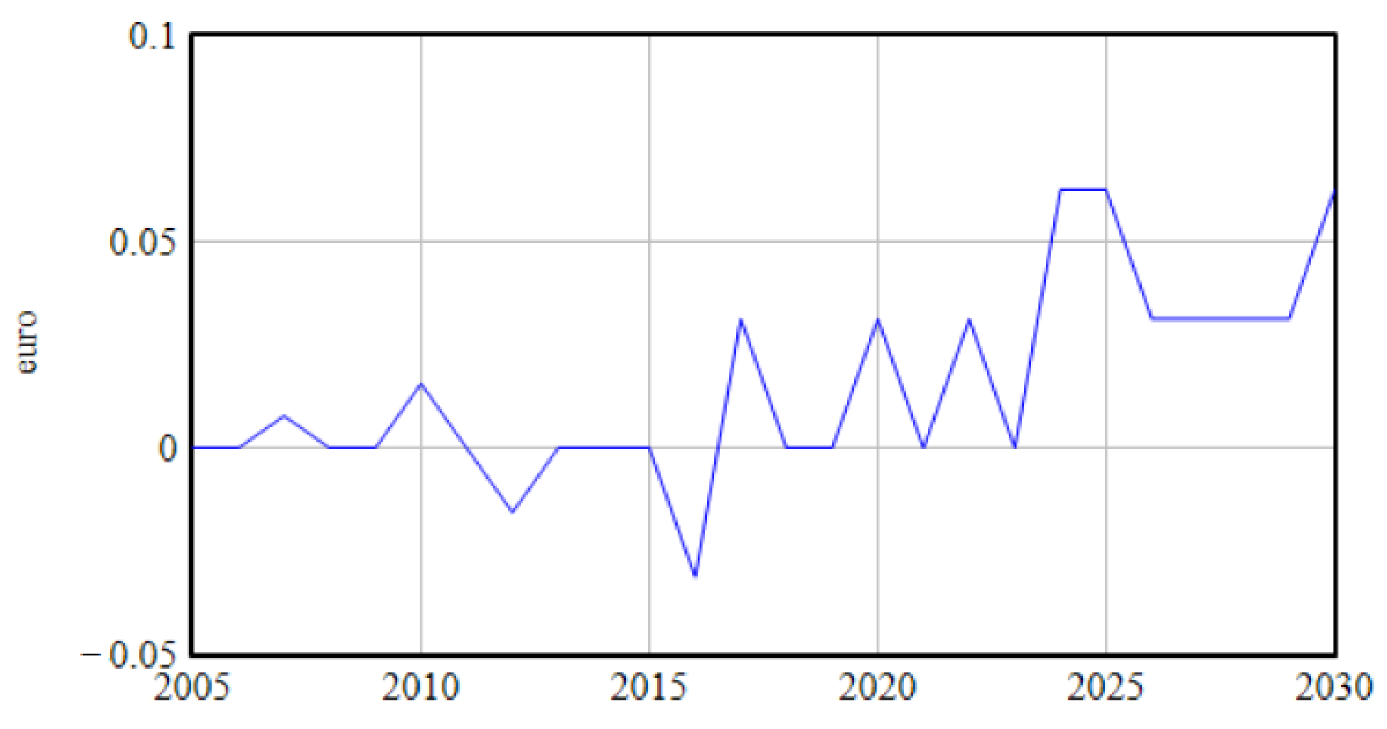
Two SFC tests are performed, one for each individual agent (i.e., assets and liabilities match within every agent at every point in time), and a second one at the system level (i.e., financial institutions’ liabilities match the liquidity in the entire economy). Concerning the second test, which determines whether consistency at the system level (i.e., for all the agents involved) is attained, the results are shown in Figure A1. The deviations from zero in our checks (visible in Figure A1 and available also in the model) are rather small, that is, within EUR 0.1, out of the large numbers used to initialize the stock and cash flow variables to several billion Euros, as indicated in Table 2 and Table 3). This also partially works as an integration test in the model. This SD model is a continuous time model adopting Euler type integration at time steps of 0.25 years. Due to the stock calculation inherent in the software, the system makes tiny approximations of the large numbers that have been used to run the model. The tiny unbalances, shown in Figure A1, are simply due to this, and we can consider these as 0, thus satisfying the SFC condition.
Figure A1.
Outcome of the SFC check.
The integration error test was also performed in line with the standard SD literature, thus demonstrating that behaviour does not change below a certain delta time, and minimising the computation power to run the simulation to the minimum possible [28]. Systems boundary adequacy and structure assessment tests were carried out during the phase of construction of the model on an iterative basis, and the test for unit consistency was passed with the completed version of the model.
References
- Harrison, G.; Thiel, C.; Jones, L. Powertrain Technology Transition Market Agent Model (PTTMAM): An Introduction; Publications Office of the European Union: Luxembourg, 2016. [Google Scholar]
- European Union. Regulation (EU) 2019/631 of the European Parliament and of the Council of 17 April 2019 Setting CO2 Emission Performance Standards for New Passenger Cars and for New Light Commercial Vehicles. 2019. Available online: https://eur-lex.europa.eu/legal-content/EN/TXT/?uri=CELEX%3A32019R0631 (accessed on 1 December 2022).
- Joint Research Centre. Powertrain Technology Transition Market Agent Model (PTTMAM). 2022. Available online: https://joint-research-centre.ec.europa.eu/scientific-tools-and-databases/powertrain-technology-transition-market-agent-model-pttmam/powertrain-technology-transition-market-agent-model-pttmam_en (accessed on 1 December 2022).
- Daimler. Annual Report 2020; Daimler AG: Stuttgart, Germany, 2021. [Google Scholar]
- Volkswagen. Annual Report 2020; Volkswagen (VW) AG: Wolfsburg, Germany, 2021. [Google Scholar]
- European Investment Bank. European Investment Bank (EIB). 2021. Available online: www.eib.org (accessed on 1 December 2022).
- Lam, A.; Mercure, J.-F. Which policy mixes are best for decarbonising passenger cars? Simulating interactions among taxes, subsidies and regulations for the United Kingdom, the United States, Japan, China, and India. Energy Res. Soc. Sci. 2021, 75, 101951. [Google Scholar] [CrossRef]
- Mercure, J.-F.; Salas, P.; Vercoulen, P.; Semieniuk, G.; Lam, A.; Pollitt, H.; Holden, P.B.; Vakilifard, N.; Chewpreecha, U.; Edwards, N.R.; et al. Reframing incentives for climate policy action. Nat. Energy 2021, 6, 1133–1143. [Google Scholar] [CrossRef]
- Jochem, P.; Gómez Vilchez, J.J.; Ensslen, A.; Schäuble, J.; Fichtner, W. Methods for forecasting the market penetration of electric drivetrains in the passenger car market. Transp. Rev. 2018, 38, 322–348. [Google Scholar] [CrossRef] [Green Version]
- Gómez Vilchez, J.J.; Jochem, P. Simulating vehicle fleet composition: A review of system dynamics models. Renew. Sustain. Energy Rev. 2019, 115, 109367. [Google Scholar] [CrossRef]
- Gómez Vilchez, J.J.; Jochem, P.; Fichtner, W. Interlinking major markets to explore electric car uptake. Energy Policy 2020, 144, 111588. [Google Scholar] [CrossRef]
- Gómez Vilchez, J.J.; Thiel, C. Simulating the battery price and the car-mix in key electro-mobility markets via model coupling. J. Simul. 2020, 14, 242–259. [Google Scholar] [CrossRef]
- Cavana, R.Y.; Dangerfield, B.C.; Pavlov, O.V.; Radzicki, M.J.; Wheat, I.D. Feedback Economics: Economic Modeling with System Dynamics; Springer International Publishing: Berlin/Heidelberg, Germany, 2021. [Google Scholar]
- Godley, W.; Lavoie, M. Monetary Economics: An Integrated Approach to Credit, Money, Income, Production and Wealth; Palgrave Macmillan: London, UK, 2007. [Google Scholar]
- Pasqualino, R.; Jones, A.W. Resources, Financial Risk and the Dynamics of Growth: Systems and Global Society; Taylor & Francis: Abingdon, UK, 2020. [Google Scholar]
- Battiston, S.; Monasterolo, I.; Riahi, K.; van Ruijven, B.J. Accounting for finance is key for climate mitigation pathways. Science 2021, 372, 918–920. [Google Scholar] [CrossRef] [PubMed]
- Dunz, N.; Naqvi, A.; Monasterolo, I. Climate sentiments, transition risk, and financial stability in a stock-flow consistent model. J. Financ. Stab. 2021, 54, 100872. [Google Scholar] [CrossRef]
- Xing, X.; Pan, H.; Deng, J. Carbon tax in a stock-flow consistent model: The role of commercial banks in financing low-carbon transition. Financ. Res. Lett. 2022, 50, 103186. [Google Scholar] [CrossRef]
- Sanders, M.; Serebriakova, A.; Fragkos, P.; Polzin, F.; Egli, F.; Steffen, B. Representation of financial markets in macro-economic transition models—A review and suggestions for extensions. Environ. Res. Lett. 2022, 17, 083001. [Google Scholar] [CrossRef]
- Sanz, R.A.; Arias, J.G.; Fidalgo, J.M.G.; García, R.M. Finanzas Empresariales; Centro de Estudios Ramón Areces: Madrid, Spain, 2016. [Google Scholar]
- Koo, R.C. The Holy Grail of Macroeconomics: Lessons from Japan’s Great Recession; Wiley: Hoboken, NJ, USA, 2011. [Google Scholar]
- KPMG. IFRS® Compared to US GAAP; KPMG International Limited: Amstelveen, The Netherlands, 2020. [Google Scholar]
- Ittelson, T. Financial Statements: A Step-by-Step Guide to Understanding and Creating Financial Reports; CAREER Press: Wayne, NJ, USA, 2020. [Google Scholar]
- Berk, J.; DeMarzo, P. Corporate Finance; Pearson: London, UK, 2019. [Google Scholar]
- Yamaguchi, K. Money and Macroeconomic Dynamics—Accounting System Dynamics Approach; Japan Futures Research Center: Awaji Island, Japan, 2020; Available online: http://www.muratopia.org/Yamaguchi/MacroBook.html (accessed on 10 February 2023).
- Bossel, H. Systems and Models: Complexity, Dynamics, Evolution, Sustainability; BoD—Books on Demand: Norderstedt, Germany, 2007. [Google Scholar]
- Sterman, J.D. Business Dynamics: Systems Thinking and Modeling for a Complex World; McGraw-Hill/Irwin: Boston, MA, USA, 2000. [Google Scholar]
- López, B.B.; Julve, V.M. Fundamentos de Contabilidad Financiera; Ediciones Pirámide: Madrid, Spain, 2021. [Google Scholar]
- Requeijo, J.; González, J.R. Técnicas Básicas de Estructura Económica; Delta Publicaciones: Kiel, WI, USA, 2007. [Google Scholar]
- Wheat, I.D. The feedback method of teaching macroeconomics: Is it effective? Syst. Dyn. Rev. 2007, 23, 391–413. [Google Scholar] [CrossRef]
- International Energy Agency. Global EV Data Explorer; International Energy Agency (IEA): Paris, France, 2021; Available online: https://www.iea.org/articles/global-ev-data-explorer (accessed on 1 December 2022).
- International Energy Agency. Global EV Outlook 2022; International Energy Agency (IEA): Paris, France, 2022. [Google Scholar]
- Blatcher, R. Distributor Markup and Profit Margins in the Supply Chain. PROS. 2018. Available online: https://pros.com/learn/blog/distributor-pricing-profit-margins-pricing-markups (accessed on 1 December 2022).
- Organización de Consumidores y Usuarios. Los coches más fiables; Organización de Consumidores y Usuarios (OCU), 2022. Available online: https://www.ocu.org/coches/coches/noticias/coches-mas-fiables (accessed on 1 December 2022).
- Eurofinas. Annual Survey 2021; Eurofinas: Brussels, Belgium, 2022. [Google Scholar]
- Pierson, K. Operationalizing Accounting Reporting in System Dynamics Models. Systems 2020, 8, 9. [Google Scholar] [CrossRef] [Green Version]
- Wells, P.E. The Automotive Industry in an Era of Eco-Austerity: Creating an Industry as If the Planet Mattered; Edward Elgar: Cheltenham, UK, 2010. [Google Scholar]
- Graham, B.; Dodd, D.L.F. Security Analysis: The Classic 1951 Edition; McGraw-Hill Education: New York, NY, USA, 2005. [Google Scholar]
- de Haan, J.; Oosterloo, S.; Schoenmaker, D. Financial Markets and Institutions; Cambridge University Press: Cambridge, UK, 2015. [Google Scholar]
- European Investment Bank. Energy Crisis Makes Public Banks Even More Important; European Investment Bank (EIB), 2022. Available online: https://www.eib.org/en/stories/energy-crisis-net-zero-transition?utm_source=mailjet&utm_medium=Email&utm_campaign=november&utm_content=na (accessed on 1 December 2022).
- Bayerische Motoren Werke. Annual Report 2019; Bayerische Motoren Werke (BMW) AG: Munich, Germany, 2020. [Google Scholar]
- Stigum, M.; Crescenzi, A. Stigum’s Money Market, 4E; McGraw Hill LLC: New York, NY, USA, 2007. [Google Scholar]
- McKinsey. In The Rise and Rise of the Global Balance Sheet—How Productively Are We Using Our Wealth? McKinsey Global Institute: Washington, DC, USA, 2021.
- European Central Bank. Annual Consolidated Balance Sheet of the Eurosystem; European Central Bank (ECB), 2022. Available online: https://www.ecb.europa.eu/pub/annual/balance/html/index.en.html (accessed on 1 December 2022).
- European Investment Bank. Shareholders. Shareholders; European Investment Bank (EIB), 2022. Available online: https://www.eib.org/en/about/governance-and-structure/shareholders/index.htm (accessed on 1 December 2022).
- International Monetary Fund. Public Sector Balance Sheet (PSBS) Database; International Monetary Fund (IMF), 2022. Available online: https://data.imf.org/?sk=82A91796-0326-4629-9E1D-C7F8422B8BE6 (accessed on 1 December 2022).
- Martinez-Moyano, I.J. Documentation for model transparency. Syst. Dyn. Rev. 2012, 28, 199–208. [Google Scholar] [CrossRef]
Figure 1.
PTTMAM’s market agents, their decisions and linkages (Source: [3]).
Figure 1.
PTTMAM’s market agents, their decisions and linkages (Source: [3]).
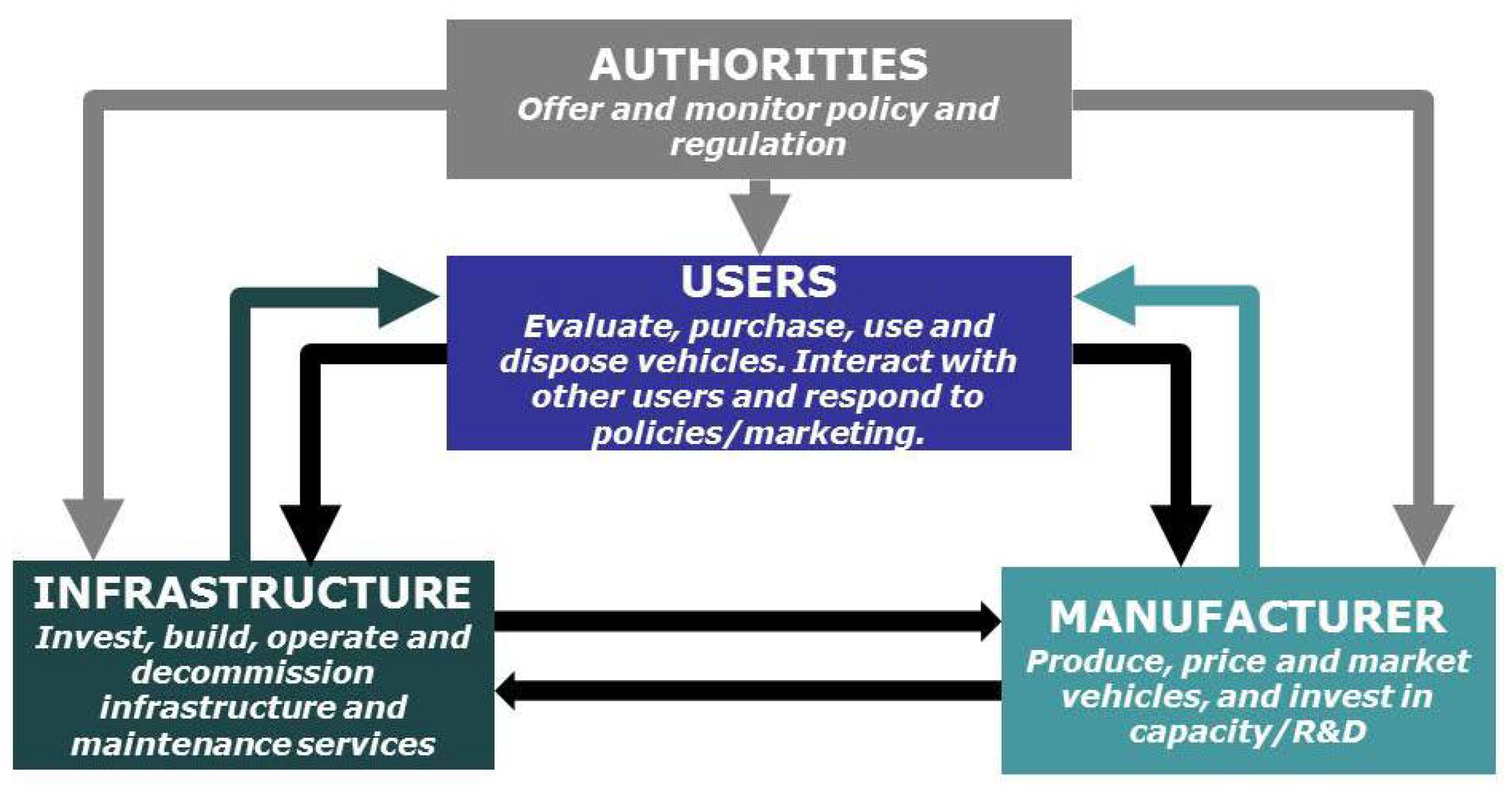
Figure 2.
Overview of the conceptual model, with interactions among agents.

Figure 3.
Causal loop diagram with feedback processes involving three agents.
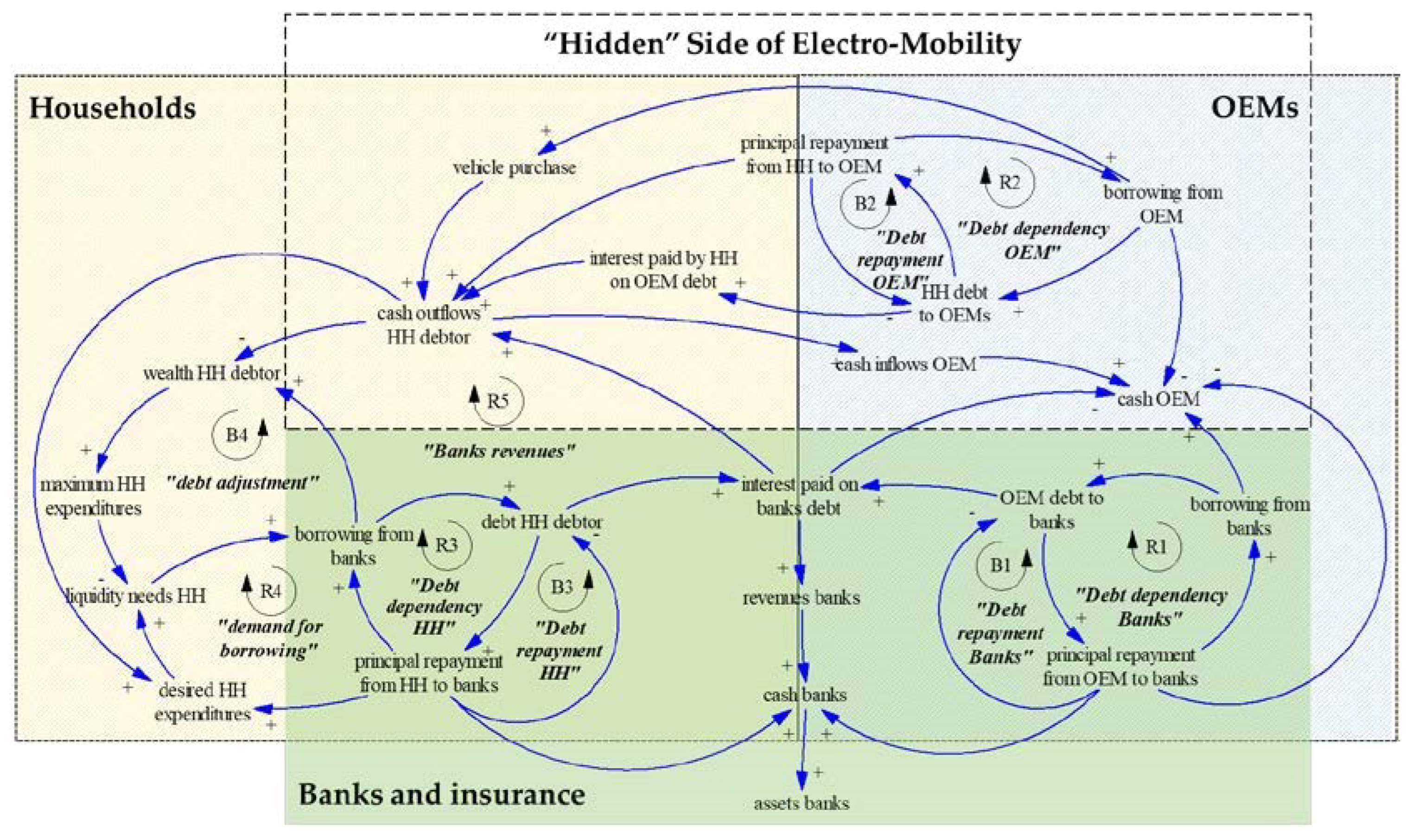
Figure 4.
Overview of the ECB structure in the model. Note: the rectangles represent stock variables; flow variables are represented by valves and pipes.
Figure 4.
Overview of the ECB structure in the model. Note: the rectangles represent stock variables; flow variables are represented by valves and pipes.
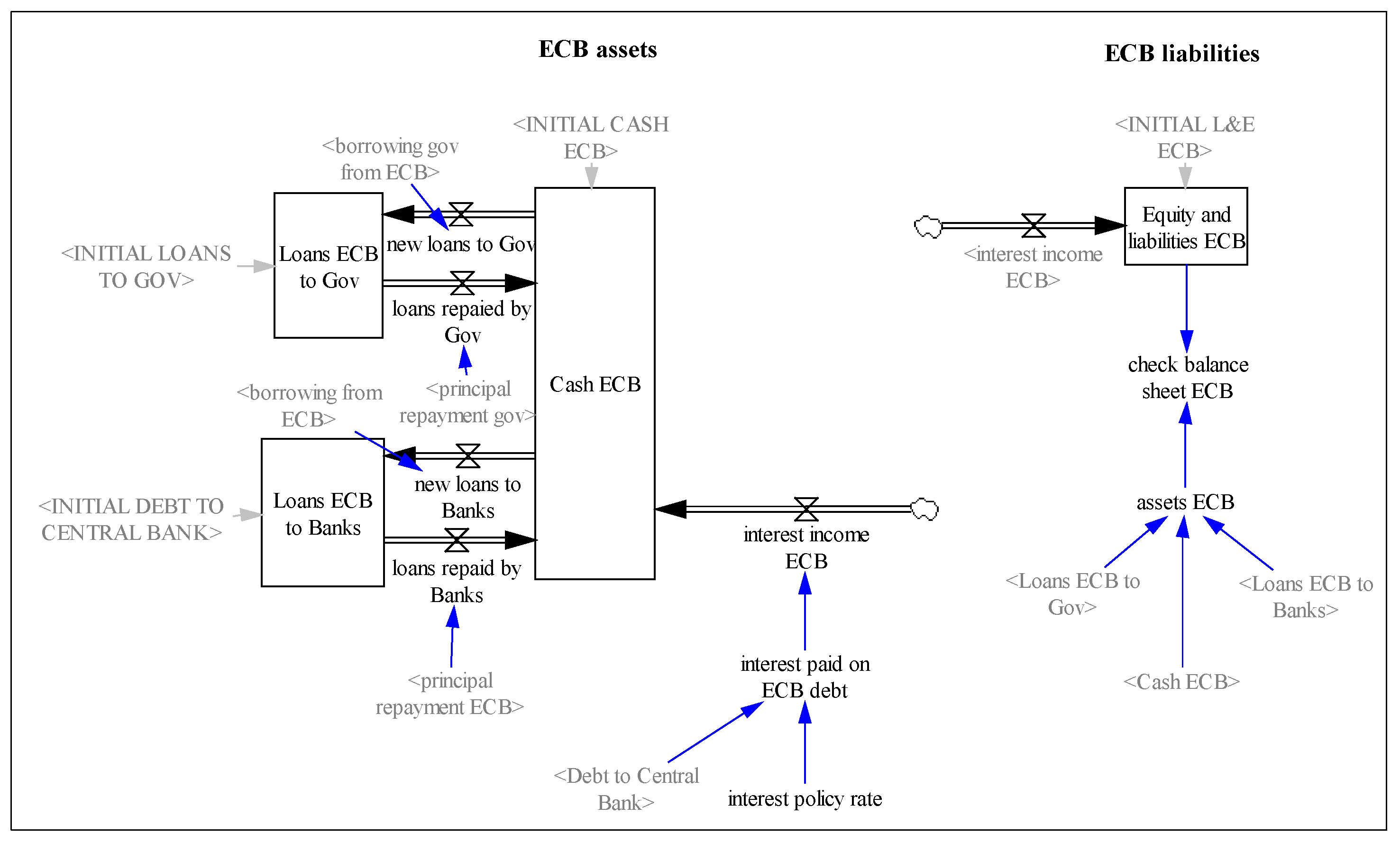
Figure 5.
Simulated vehicle stock (2005–2030), by type of vehicle and powertrain (a) cars, (b) vans, (c) trucks, (d) buses.
Figure 5.
Simulated vehicle stock (2005–2030), by type of vehicle and powertrain (a) cars, (b) vans, (c) trucks, (d) buses.
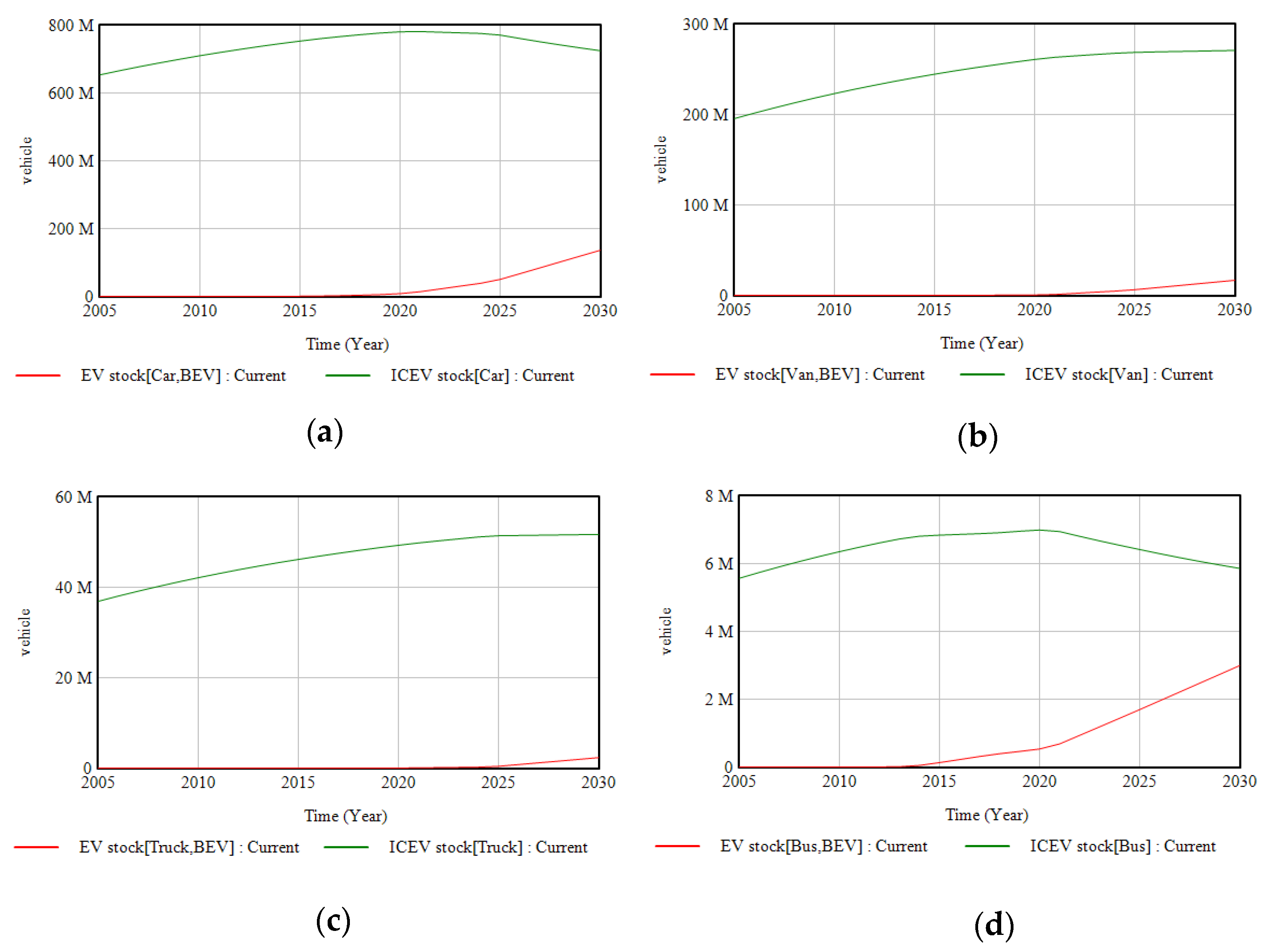
Figure 6.
Balance sheet simulation of: (a) public banks; (b) private banks and government.

Figure 7.
Balance sheet simulation of: (a) households; (b) firms.

Table 1.
European Investment Bank’s finance support to the automotive sector: selected results on R&D and EV production.
Table 1.
European Investment Bank’s finance support to the automotive sector: selected results on R&D and EV production.
| Year | Name/Area | Firm | Finance [EURmio] |
|---|---|---|---|
| 2010 | R&D trucks | Daimler | 400 |
| 2010 | Environmentally friendly vehicles | Ford | 450 * |
| 2010 | EV and battery production | Nissan | 220 |
| 2011 | Research to meet emission targets | Fiat | 250 |
| 2011 | Hybridisation | BMW | 325 |
| 2011 | R&D (electrification) | Renault | 180 |
| 2012 | R&D (emissions/safety) | Daimler | 300 |
| 2013 | Innovative technologies | BMW | 400 |
| 2013 | Research to meet emission targets | Renault | 400 |
| 2013 | FCEV | Daimler | 400 |
| 2014 | R&D trucks | Daimler | 500 |
| 2014 | Innovative powertrains | VW | 500 |
| 2015 | R&D (efficient engines) | FCA | 600 |
| 2016 | R&D (alternative fuel/hybrid engines) | FCA | 250 |
| 2017 | Innovative powertrains | PSA | 250 |
| 2017 | R&D (hybrid/electric) | Volvo Cars | 245 |
| 2018 | Hybrid and electric vehicles | FCA | 420 |
| 2019 | Electric motor development | PSA/NIDEC | 145 |
| 2020 | EV (BEV/PHEV) production | FCA (Stellantis) | 300 |
| 2020 | PHEV production/R&D (automation) | FCA (Stellantis) | 485 |
* GBP. Source: own collection from [6].
Table 3.
Initial values of the Banks and insurance’ balance sheets [EUR].
| Balance Sheet Item | From OEM (Automotive) | From OEM (Financial) |
|---|---|---|
| Cash and cash equivalents | 1011 | |
| Loans to consumers | 7.87 × 10¹² | |
| OEM debt (short-term) | 1.25 × 10¹¹ | 7.21 × 10¹¹ |
| OEM debt (long-term) | 1.73 × 10¹¹ | 1.02 × 10¹² |
| Deposits | 4.5 × 10¹² | |
| Debt to central bank Equity | 4.5 × 10¹² 1012 | |
| Assets | 1013 | |
| Liabilities and equity | 1013 | |
Source: own assumptions.
Table 4.
Initial values of the HHs’ balance sheets [EUR].
| Balance Sheet Item | Creditor | Debtor |
|---|---|---|
| Wealth (assets) | 4.5 × 10¹² | 9.04 × 10¹² |
| Bank loans | 0 | 7.87 × 10¹² |
| Debt to OEM (short-term) | 0 | 5.19 × 10¹¹ |
| Debt to OEM (long-term) | 0 | 6.51 × 10¹¹ |
| Equity | 4.5 × 10¹² | 0 |
| Assets | 1.35 × 10¹³ | |
| Liabilities and equity | 1.35 × 10¹³ | |
Source: own assumptions.
Table 5.
Initial values of the OEMs’ balance sheet [EUR].
| Balance Sheet Item | Automotive Division | Financial Division |
|---|---|---|
| Cash and cash equivalents | 9.73 × 10¹⁰ | 1.10 × 10¹⁰ |
| Securities | 8.43 × 10¹⁰ | 5.52 × 10⁹ |
| Trade receivables | 5.51 × 10¹⁰ | 0 |
| Financial services receivables | 0 | 2.60 × 10¹¹ |
| Inventories | 8.75 × 10¹⁰ | 0 |
| Property, plant & equipment | 2.16 × 10¹¹ | 0 |
| Intangibles | 2.40 × 10¹⁰ | 0 |
| Leases | 0 | 1.40 × 10¹¹ |
| Financial services noncurrent | 0 | 3.26 × 10¹¹ |
| Trade payables | 1.07 × 10¹¹ | 0 |
| Debt (short-term) | 6.27 × 10¹⁰ | 3.60 × 10¹¹ |
| Debt (long-term) | 8.96 × 10¹⁰ | 5.08 × 10¹¹ |
| Retained earnings | 1.55 × 10¹¹ | |
| Reserves | 2.31 × 10¹⁰ | |
| Assets | 1.31 × 10¹² | |
| Liabilities and equity | 1.31 × 10¹² | |
Source: own assumptions as a result of simplifying and aggregating the information contained in publicly available financial statements, as reported by several OEMs.
Table 6.
Further model assumptions for OEMs.
| Constant/Variable | Value | Justification |
|---|---|---|
| Administrative intensity | 4% | Own analysis 1 |
| Corporate tax rate | 30% | [5] (p. 128) |
| Dividend distribution ratio | 40% | [4] (p. 133) |
| Emission penalties | EUR 0 | Assuming targets are met |
| Lifetime plant | 50 yr | Values range up to 60 yr |
| Lifetime vehicle | 5 yr | Values range up to 10 yr |
| Marketing intensity | 10% | Own analysis 1 |
| R&D intensity | 6% | Own analysis 1 |
| Revenues from leasing | EUR 4900/car | Own assumption |
| Spread over APR | 1% | Own assumption |
1 Forthcoming. ‘Intensity’ is relative to sales revenues. Lifetime values sourced from OEM reports.
Table 7.
Assumptions, by type of vehicle.
| Constant/Variable | Unit | Car | Van | Truck | Bus |
|---|---|---|---|---|---|
| Battery capacity 1 | kWh | 24/30/50 | 24/30/50 | 300 | 250 |
| Labour cost | EUR/vehicle | 5000 | 3750 | 25,000 | 50,000 |
| Material cost [BEV] | EUR/vehicle | 7845 | 4095 | 32,069 | 114,224 |
| Material cost [ICEV] | EUR/vehicle | 5000 | 3750 | 25,000 | 50,000 |
| Annual mileage | km/vehicle | 12,000 | 24,000 | 80,000 | 110,000 |
| Fuel efficiency [BEV] | kWh/km | 0.2 | 0.2 | 1.3 | 1.3 |
| Fuel efficiency [ICEV] | litre/km | 0.08 | 0.08 | 0.36 | 0.36 |
1 The first value is used for 2005–2014, the second for 2015–2019 and the third for 2020–2030.
Table 8.
Simulated values of the financial KPIs and benchmarks.
| KPI | Simulated 1 | 25% | Median | 75% |
|---|---|---|---|---|
| Gross margin | 42/37% | 28% | 43% | 63% |
| Operating margin | 20/16% | 6% | 12% | 22% |
| EBIT margin | 20/16% | 5% | 11% | 18% |
| Net profit margin | 13/11% | 2% | 7% | 15% |
| ROE | 7/4% | 3% | 10% | 18% |
1 These are our model results, with the first value corresponding to 2005 and the second to 2030. The values for the last three columns correspond to quartiles from large US firms in 2018 and were sourced from Table 2.4 in [24].
Disclaimer/Publisher’s Note: The statements, opinions and data contained in all publications are solely those of the individual author(s) and contributor(s) and not of MDPI and/or the editor(s). MDPI and/or the editor(s) disclaim responsibility for any injury to people or property resulting from any ideas, methods, instructions or products referred to in the content. |
© 2023 by the authors. Licensee MDPI, Basel, Switzerland. This article is an open access article distributed under the terms and conditions of the Creative Commons Attribution (CC BY) license (https://creativecommons.org/licenses/by/4.0/).
Share and Cite
MDPI and ACS Style
Gómez Vilchez, J.J.; Pasqualino, R. The Hidden Side of Electro-Mobility: Modelling Agents’ Financial Statements and Their Interactions with a European Focus. Systems 2023, 11, 132. https://doi.org/10.3390/systems11030132
AMA Style
Gómez Vilchez JJ, Pasqualino R. The Hidden Side of Electro-Mobility: Modelling Agents’ Financial Statements and Their Interactions with a European Focus. Systems. 2023; 11(3):132. https://doi.org/10.3390/systems11030132
Chicago/Turabian StyleGómez Vilchez, Jonatan J., and Roberto Pasqualino. 2023. "The Hidden Side of Electro-Mobility: Modelling Agents’ Financial Statements and Their Interactions with a European Focus" Systems 11, no. 3: 132. https://doi.org/10.3390/systems11030132
Note that from the first issue of 2016, this journal uses article numbers instead of page numbers. See further details here.