
Real-Time Scheduling of Pumps in Water Distribution Systems Based on Exploration-Enhanced Deep Reinforcement Learning

1
School of Environment, Harbin Institute of Technology, Harbin 150090, China
2
Guangdong Yuehai Water Investment Co., Ltd., Shenzhen 518021, China
3
National Engineering Research Center of Urban Water Resources Co., Ltd., Harbin Institute of Technology, Harbin 150090, China
*
Author to whom correspondence should be addressed.
Systems 2023, 11(2), 56; https://doi.org/10.3390/systems11020056
Submission received: 13 December 2022
/
Revised: 11 January 2023
/
Accepted: 18 January 2023
/
Published: 20 January 2023
(This article belongs to the Section Cybernetics)
Abstract
:Effective ways to optimise real-time pump scheduling to maximise energy efficiency are being sought to meet the challenges in the energy market. However, the considerable number of evaluations of popular optimisation methods based on metaheuristics cause significant delays for real-time pump scheduling, and the simplification of traditional deterministic methods may introduce bias towards the optimal solutions. To address these limitations, an exploration-enhanced deep reinforcement learning (DRL) framework is proposed to address real-time pump scheduling problems in water distribution systems. The experimental results indicate that E-PPO can learn suboptimal scheduling policies for various demand distributions and can control the application time to 0.42 s by transferring the online computation-intensive optimisation task offline. Furthermore, a form of penalty of the tank level was found that can reduce energy costs by up to 11.14% without sacrificing the water level in the long term. Following the DRL framework, the proposed method makes it possible to schedule pumps in a more agile way as a timely response to changing water demand while still controlling the energy cost and level of tanks.
1. Introduction
Water distribution systems (WDSs) represent vast and complex infrastructures that are essential for residents’ lives and industrial production. Water utilities are committed to providing customers with sufficient water of the required quantity by operating WDSs. The corresponding energy cost of pumps constitutes the dominant expenditure of the operational cost of a WDS [1,2,3,4]. However, the energy market is experiencing great challenges. Extreme climate [5], economic crises [6], war [7], and public health events (such as the COVID-19 pandemic) [8,9] have produced huge negative shocks in the energy market, making it full of uncertainties and fluctuations. These challenges in the energy market have large implications for water utilities. On the one hand, the high operating cost caused by rising energy prices directly affects the financial health of water utilities. On the other hand, a significant energy shortage would make the pumping or treatment of water impossible [10]. Hence, it is an important issue for water utilities to improve the energy efficiency of pumps and integrate water supply strategies and energy conservation goals.
The problem of finding the optimum pump schedule is far from simple; both the hourly water demand of consumers and electricity tariffs can vary greatly during the scheduling period. Minimum and maximum levels of tanks are hard constraints that must be satisfied to guarantee the reliability of the supply, and the desired pressures should be maintained for consumers. In addition to these factors, the hydraulic formulas of WDSs are highly nonlinear and complex, making computer modelling a difficult and very time-consuming process.
Various optimisation methods have been applied to pump scheduling problems. Deterministic methods are used initially, including linear [11], nonlinear [12,13,14], dynamic [15,16], and mixed-integer programming [17,18]. Most of these methods simplify the complexities and interdependencies of WDSs by assumptions, discretisation, or heuristic rules [1,13,19]. Although these simplifications can make it easier to address the problem, they may introduce bias and exclude potentially good solutions. In the mid-1990s, stochastic optimisation methods (metaheuristics) were introduced to pump scheduling optimisation problems [20], such as the genetic algorithm (GA) [21,22,23,24], particle swarm optimisation (PSO) [25,26], and differential evolution (DE) [27]. These metaheuristics do not require simplification of the hydraulic models and have proven to be robust, even for highly nonlinear and nondifferentiable problems. However, metaheuristics require a large number of evaluations to achieve convergence, which requires too much time for real-time processing.
In recent years, the development of machine learning has introduced opportunities for the scientific management of water utilities. Various machine learning methods are used in a wide variety of applications, from anomaly detection [28,29] through system prediction [30,31,32] to system condition assessment [33] and system operation [34,35,36].
In scheduling problems, machine learning techniques are usually used as surrogate models of WDSs in metaheuristic optimisation to save computational load. Broad et al. [37] used an artificial neural network (ANN) as a metamodel, which can approximate the nonlinear functions of a WDS and provide good approximation for simulation models. However, how to reduce the error of surrogate models and ensure that the solution is still optimal compared with a full complex network simulator remains unknown.
Deep reinforcement learning (DRL) is a promising method for nonlinear and nonconvex optimisation problems. The essence of DRL is the combination of reinforcement learning (RL) and deep learning. It has been explored widely in recent years with the appearance of AlphaGo [38]. However, its application in pump scheduling problems is still very limited. In 2020, Hajgató et al. [39] applied DRL to the single-step pump scheduling problem and took the results of the Nelder–Mead method as the reward standard. An essential contribution of Hajgató et al. is that the method models the single-step real-time pump scheduling problem as a Markov decision process (MDP) and considers multiple objectives, including satisfaction of consumers, efficiency of the pumps, and the feed ratio of the water network. However, the method sacrifices the regulation and storage capacity of the tanks and takes the pump speeds obtained by the Nelder–Mead method as the optimal setting, which makes the DRL results depend largely on the Nelder–Mead method.
Based on the above literature review of pump scheduling optimisation in WDSs, there are three main limitations for real-time pump scheduling problems: heavy computational loads, a lack of accuracy for surrogate models, and a lack of proper usage of the storage capacity of tanks. Real-time pump scheduling based on reinforcement learning is presented in this paper. The main contributions of this paper are as follows:
First, an RL environment of the pump scheduling problem was constructed using a full network simulator, and the computation-intensive task was transferred from online to offline to save application time.
Second, by constructing a reward function, the penalty form of the tank level was explored to reduce the energy cost and maintain the tank level in the long term.
Finally, an exploration-enhanced reinforcement learning framework was proposed, adding an entropy bonus to the policy objective. The results demonstrate that compared with metaheuristics, the proposed method can obtain suboptimal scheduling policies under various demand distributions within one second.
The rest of the paper is organised as follows. In Section 2, we introduce the details of DRL, proximal policy optimisation (PPO), the exploration enhancement method, and the designs of important factors for applying DRL in pump scheduling problems. In Section 3, the reinforcement learning method is applied to a WDS case, the results are presented, and key findings are analysed. Section 4 concludes this paper.
2. Methods
2.1. Reinforcement Learning (RL)
The RL algorithm is used to solve the sequence decision problem and can mathematically be formulated as a Markov decision process (MDP). The training process of RL is carried out through the interaction between the agent and environment. At time step , the agent executes an action () according to the current state () and the policy function, obtaining an immediate reward (); then, the environment transfers to the next time step state (). The agent adjusts its policy through the experience collected in the interaction process. After a large number of interactions with the environment, an agent with an optimal policy is obtained. Then, the trained policy neural network can be used for pump scheduling. Compared with other optimisation methods such as GA, the RL method divides the optimisation process into training and application, which can transfer the computationally intensive training process from online to offline to achieve real-time scheduling applications. The learned policy of RL is also able to handle the uncertainty of the environment, such as the uncertainty of demand, as the learned policy neural network is obtained by interactions with the environment under a large number different states with uncertainty.
The MDP can be represented by a tuple, <S, A, P, R, γ >, where:
- S is the state space, which is a set of states;
- A is the action space, which is a set of executable actions for the agent;
- P is the transition distribution, which describes the probability distribution of the next time step state under different and ;
- R is the reward function, is the step reward after the agent takes an under state ; and
- is the discount factor used to calculate the cumulative reward (), which is defined as:
2.2. Design of Significant Factors for RL Application to Pump Scheduling
In the following, the most significant factors in RL, namely S, A, and R, are discussed in detail for application to optimal real-time pump scheduling in WDSs.
2.2.1. State Space
State space is a set of all possible states in the environment. The state consists of relevant information for the agent to learn the optimal policy. This means that the state should contain enough effective information of the current environment. However, excess information may lead to confusion for the agent during the process of assigning rewards to the state. Therefore, it is important to properly select the state space in the RL application. For this work, the pump scheduling information in the WDS was divided into two categories: the water demand of consumers and the status information of the tank levels.
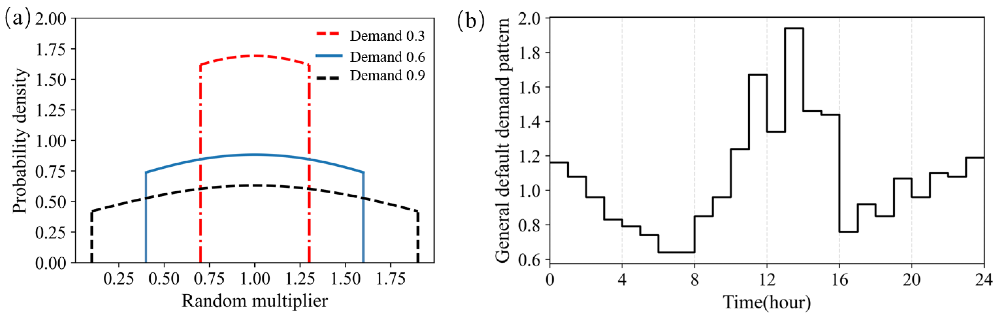
To make the built environment approach the actual WDS, the uncertainty of water demand in the real world was considered. The randomisation of water demand in the environment was carried out in two steps to mimic the time and space effects. Firstly, the general default demand pattern (as shown in Figure 1b) was multiplied by hourly random multipliers to simulate the random fluctuation of hourly water demand. Secondly, the base demand was obtained by the product of the nodal random multiplier and the default base demand. The demand with uncertainty was generated in every general node as the product of the pattern and base demand constructed above. Both random multipliers of time and space follow the truncated normal distribution. The truncated normal distribution has its domain (the random multiplier) restricted to a certain range of values, such as . To simplify, the random multipliers of time and space are limited to the same range, and the water demand distribution of which the space and time random multiplier ranges are (1 − ∆, 1 + ∆) is called demand (∆) hereafter. The probability density distributions of the truncated normal distribution of the random multiplier for demand 0.3, demand 0.6, and demand 0.9 are shown as examples in Figure 1a. For a large consumer, we consider it a node with less uncertainty compared to the general consumer and do not apply a randomisation method to it.
The initial water levels of the tanks follow a uniform distribution of (0, 1). Then, the following tank levels are calculated according to the state and action.
2.2.2. Action Space
Action is defined as the relative pump speed, which is the ratio of the pump speed compared to the nominal pump speed. The pumps in a WDS are considered variable-speed pumps. The trained agent selects the optimal pump speed from all combinations of pump speeds for every time interval of the scheduling period under the guidance of the learned strategy. Each relative pump speed is considered a discrete variable ranging from 0.7 to 1.0, with an increase of 0.05 due to mechanical limitation. The size of the action space grows exponentially with an increase in the number of pumps.
2.2.3. Reward Function
The reward function is defined to motivate the agent to achieve its goal. The value of the reward represents the quality of the action. For this work, the reward function consists of three important parts: the energy cost of pumps (), the penalty for hydraulic constraints (), and the penalty for tank-level variation (). The reward value is calculated according to Algorithm 1.
- (1)
- Energy cost of pumps
The essential goal of the real-time pump scheduling optimisation method proposed in this work is to minimize the energy cost of pumps while fulfilling system constraints. The reward design of energy cost should consider two key points. First, the lower the energy cost of pumps, the higher the designed reward. Second, avoid obtaining all positive or negative rewards in the learning process, as such a strategy is not conducive to agent training. According to the above requirements, the reward of energy cost is defined as the difference between the benchmark of energy cost () and the actual energy cost (). The benchmark is to balance the positive and negative distribution of energy cost rewards. When the energy cost is lower than the benchmark, the reward is positive; otherwise, the reward is negative. The lower the energy cost, the larger the reward. The benchmark is the average energy cost obtained by the agent interacting with the environment for 20,000 episodes, making random actions.
- (2)
- Hydraulic constraint
When the hydraulic constraint (such as the pressure of nodes) cannot be fulfilled under the current action, a penalty is added to the reward function. After receiving the penalty, the agent learns that this is a bad action and adjusts the corresponding policy.
- (3)
- Tank-level variation
Tank-level variation (mainly refers to tank-level reduction in a day) should be as small as possible to avoid the agent learning to reduce the energy cost by overconsuming water in the tanks. This may lead to water shortages and extra costs of complementing water in the tanks. For these reasons, when the water volume in the tank at the end of the scheduling period () is less than the initial volume (), a negative reward is added to the reward function. Compared with the strict limit of the tank level in a day, we attempted to find a way to make full use of the storage and regulation capacity of the tanks to reduce energy cost and maintain the tank level in the long term. The form of the negative reward () has a great impact on the learned policy, as explored in Section 3.1.
| Algorithm 1 Reward function | |
| 1: | for do |
| 2: | Take action for state , collecting ,. |
| 3: | if hydraulic punishment = False then |
| 4: | if then |
| 5: | |
| 6: | else |
| 7: | if then |
| 8: | |
| 9: | else |
| 10: | |
| 11: | end if |
| 12: | end if |
| 13: | else |
| 14: | |
| 15: | break |
| 16: | end if |
| 17: | end for |
2.3. Reinforcement Learning Model
2.3.1. Proximal Policy Optimisation (PPO)
In this study, we applied the PPO algorithm [40] to determine the optimal real-time pump schedule. PPO is an on-policy RL method that updates policy with a new batch of experiences collected over time. The policy gradient method estimates the policy gradient and inputs it into gradient ascent optimisation to improve the policy. The original policy estimation has the following form:
where is the policy, and is the estimation of advantage at timestep This is a process alternating between sampling and updating. To reuse the sampled data and make the largest improvement to the policy, the probability ratio is used in PPO to support several off-policy steps. The definition of is expressed as Formula (3). Moreover, to avoid excessively large policy updates, the PPO algorithm has a clipping mechanism in the objective function, as shown in Formulas (4) and (5).
where is a hyperparameter. When the new policy is far from the old policy, , clipping removes the incentives for moving outside of the interval . The PPO training process is expressed as Algorithm 2.
| Algorithm 2 PPO | |
| 1: | , |
| 2: | for k = 0, 1, 2, …, do |
| 3: | Collect set of trajectories by running policy in the environment. |
| 4: | Compute reward-to-go based on the collected trajectories. |
| 5: | . |
| 6: | Update the policy by maximising the PPO objective: |
| 7: | by regression on mean-squared error: |
| 8: | end for |
2.3.2. Exploration Enhancement
The PPO algorithm suggests adding an entropy bonus to the objective to ensure sufficient exploration when using a neural network architecture that shares parameters between the policy and value function [40]. The objective is obtained as follows:
where is the square-error loss between the target value and the estimated value, is the entropy bonus, and and are coefficients.
In this paper, an exploration-enhanced PPO (E-PPO) based on an entropy bonus is proposed. The idea of the entropy bonus is extended to the PPO model, which does not share parameters between the policy and value function. The policy objective is obtained as Formula (7). The objective of the value function remains unchanged. Moreover, as the initial entropy is expected to be as large as possible to reduce the probability of learning failures [41,42], all the dimensions of state were normalised to maximise the initial entropy. We found that the idea of normalisation is a simple but efficient method for maximising the initial entropy.
3. Case Study: EPANet Net3
The EPANet Net3 water network was chosen as the test case to illustrate the applicability of the proposed method. This network is one of the most commonly used benchmark networks, owing to its data availability and flexibility to be modified for different optimisation problems [2]. The numerical model of the EPANet Net3 water network is accessible online in an EPANET-compatible format from the web page of the Kentucky Hydraulic Model Database for applied water distribution systems research [43].
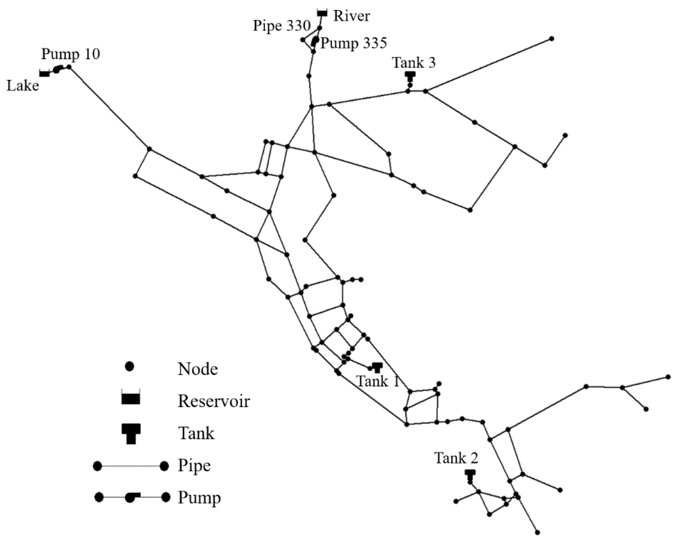
The EPANet Net3 water network is based on the North Marin Water District in Novato, CA. The network has 2 raw water sources, 2 pump stations, 3 elevated storage tanks, 92 nodes, and 117 pipes. The topology of the EPANet Net3 water network is depicted in Figure 2. The time horizon is 24 h divided into 1 h intervals for the case study.
In this study, the wire-to-water efficiency of pumps 10 and 330 was 0.75. It is worth noting that the efficiency of pumps depends on water capacity and rotation speed. In this paper, it is simplified as a fixed value. The electricity tariffs and intervals of peak and off-peak are shown in Figure 3. The peak tariff is USD 0.1194/kWh, and the off-peak tariff is USD 0.0244/kWh [44].
Some modifications were made as follows:
- (1)
- All the control rules for the lake source, pipe 330 and pump 335, were removed. In addition, pipe 330 was kept closed. This means that these two raw sources only supply water through pumps 10 and 335, which are controlled by the agent, rather than supply water under specific control rules;
- (2)
- To simulate the stochastic water demand in a real-world WDS, the randomisation method described above was used.
The epoch of metaheuristics is 100. The values of the crossover probability and mutation probability of the GA are 0.95 and 0.1, respectively. The value of the local coefficient of PSO is 1.2. For DE, the weighting factor and crossover rate are 0.1 and 0.9, respectively. The detailed settings of PPO and E-PPO in the experiments are listed in Table 1.
3.1. Effects of the Penalty Form of Tank-Level Variation
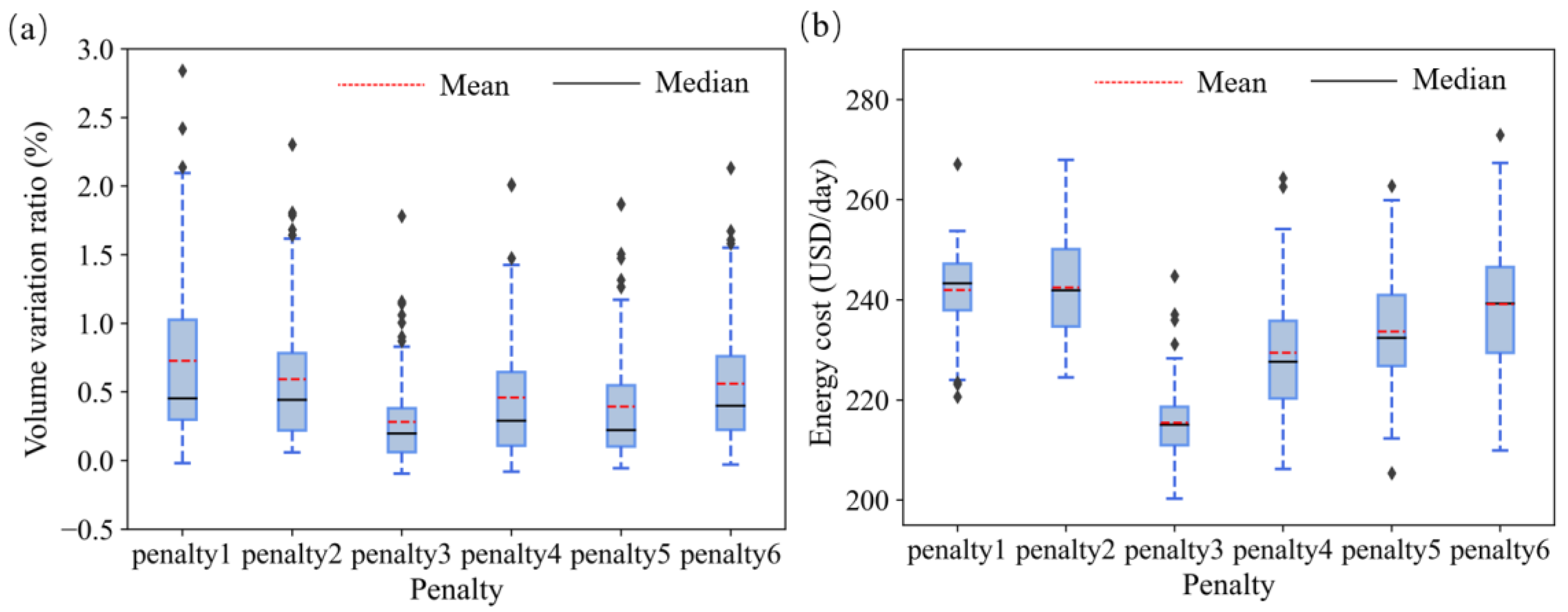
In pump scheduling problems with tanks in WDSs, the penalty form of tank-level variation must be reasonably designed to make full use of the regulation and storage capacity of the tanks to minimize the energy cost of pumps. According to Algorithm 1 described above, to achieve the goal of the agent, the penalty can be a large constant or a value that is proportional to the reduction rate of the tank level. To study the effects of penalty forms of tank-level variation on energy cost, 6 agents with different penalty forms were trained and tested on 100 random test sets. The results are shown in Figure 4. The uncertainty setting of water demand in the environment is demand 0.3, and the agent used is the PPO algorithm.
For the penalty terms of large constants, such as penalty 1 and penalty 2 in Figure 4a, almost all the cases had not lost the water in tanks at all at the end of the scheduling period. The larger the penalty value, the more conservative the agent is; that is, the agent tends to add water to the tanks as much as possible to avoid default. However, this tendency generates a high energy cost, as shown in Figure 4b. The average energy costs of penalty 1 and penalty 2 are USD 241.96/day and USD 242.45/day, respectively. For penalty forms (penalty 3 to penalty 6) that are proportional to the reduction rate of the tank level, the greater the coefficient of the penalty, the higher the energy cost, but the corresponding level of the tanks only increases slightly.
As presented in Figure 4b, penalty 3 performs best, with an average energy cost of USD 215.45/day, representing savings of 6.08% and 11.14% energy cost relative to penalty 4 and penalty 2, respectively. For penalty 3, the volume variation ratios in the tanks in most cases (Figure 4a) are positive, and the negative ratios of the few other cases are concentrated in a small area not exceeding −9.56%. However, the positive variation ratio reaches 184.93%. Suppose the 100 test cases are the states of the water distribution system for 100 different days. On most of the 100 days, the tank level rises at the end of the day. On only a few days, the level drops slightly. However, this reduction in water volume is replenished on other days when the water level rises. It can be inferred that the form of penalty 3 can reduce energy costs by up to 11.14% compared to the other five penalties without sacrificing the water level in the long term. Hence, penalty 3 was used in subsequent studies in this work for tank-level variation.
3.2. Effects of Cross Entropy
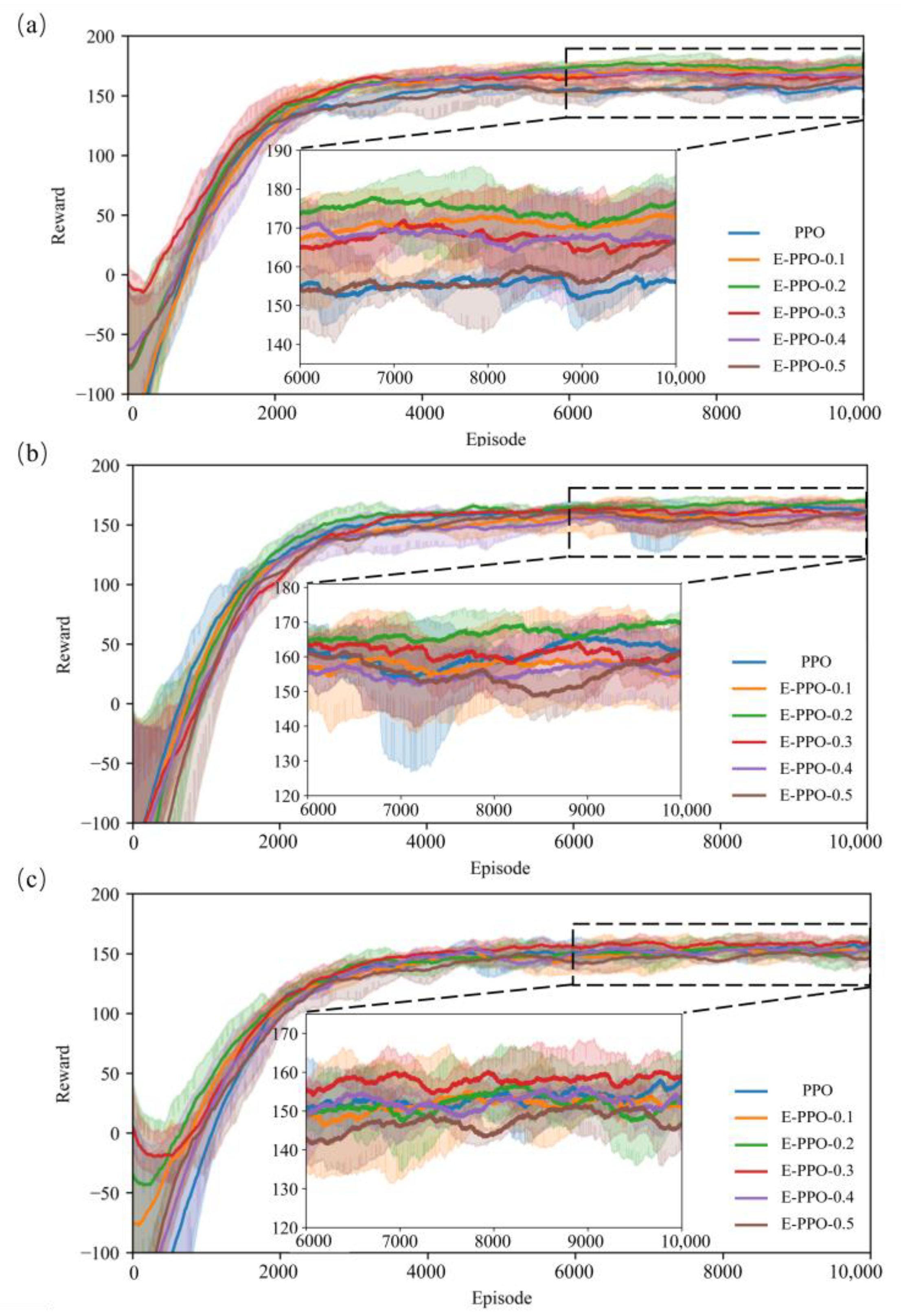
Due to the effects of sampling limitation in the experiments, the exploration range expressed by the coefficient of cross entropy () has a significant impact on the training process. In this study, we compared and verified the various settings of the coefficient of cross entropy () under different water demand distributions. Figure 5 shows the experimental results, which contain the PPO model and E-PPO model with different values of . The same experiment was conducted three times for each model. The solid line shows the average cumulative reward to eliminate the contingency of results, and the shaded part represents the reward variance for three times.
The best performance in Figure 5a reached approximately 178. Meanwhile, optimal value is 0.2. The PPO model achieved the worst performance, which may be due to the smaller exploration scope of the agent, leading to premature convergence to the suboptimal solution. When the uncertainty coefficient of water demand increases, the optimal performance of the agent decreases. The setting of 0.2 is the best, with a reward of approximately 170 for a demand uncertainty of 0.6 (Figure 5b), and the setting of 0.3 is the best with a reward of approximately 160 for a demand uncertainty of 0.9 (Figure 5c). That is because when the environment has great uncertainty, it is difficult to learn an optimal strategy network, as the state transition becomes blurred. The selection of the agent tends to be conservative. When the coefficient exceeds the optimal setting, the performance decreases as the coefficient increases (Figure 5a–c). A setting of 0.5 for the demand uncertainty of 0.6 (Figure 5b) and 0.9 (Figure 5c) shows poor performance. It may be that an entropy coefficient that is too large leads to policy degradation, which takes too much time or even cannot be optimised. Exploration ability often affects the convergence rate and final performance. Considering that tasks are often sensitive to exploration ability, it is necessary to adjust this parameter for specific tasks.
3.3. Comparison of Models
To better verify the performance and robustness of the exploration-enhanced PPO, 15 optimisation test cases were conducted under three different demand distributions in the environment. Each test case simulates 24 h of pump scheduling with a 1 h interval. The agent receives the current state of the WDN at the beginning of each hour, then executes the action of that hour online until the end of the day. The simulation period of 24 h guarantees the tank-level variation in a day, as shown in Section 2.2.3 and Section 3.1. The results were compared with metaheuristics, including GA, PSO, and DE, as shown in Table 2 and Table 3. Table 2 shows the energy cost during the scheduling period. Table 3 shows the training time and test time of the models. The PPO and E-PPO methods are trained in advance by interacting with the environment. In the application process, operators just need to call the trained model. However, the metaheuristic methods need to train the model for every single scheduling case. Simulations were carried out on a computer with an NVIDIA GeForce RTX 3070 GPU and an Intel Core i7-11700K CPU. The RL models were built by Keras, and the WDS environment was built by WNTR, which is compatible with EPANET. All the models were written in Python version 3.9.
GA converges after 100 epochs of training; therefore, the results of GA are considered as optimal solutions and benchmarks for test cases in this paper. As shown in Table 2, E-PPO exhibited optimal performance besides GA, followed by PPO, DE, and PSO, with average costs of USD 207.15/day, USD 220.60/day, USD 223.59/day, and USD 253.87/day, respectively. Compared with the optimal solution of GA, E-PPO only consumes 5.03% more energy cost on average but saves approximately 6.10% of the energy cost compared with PPO, 7.35% compared with DE, and 18.40% compared with PSO. This may be due to the fact that metaheuristics had limited performance with limited training time and parameter tuning.
Although the average training time of the E-PPO algorithm is 5495.55 s, which is longer than that of metaheuristics, it only needs 0.42 s in the scheduling process, as shown in Table 3. This is an almost negligible time consumption for hourly scheduling. However, the computation time of the GA is nearly half an hour, which is impractical for hourly scheduling. The performance of the E-PPO is only slightly worse than that of GA, but the application time cost of the E-PPO is only less than a second. As time is a very important factor in industrial production, E-PPO is a potential real-time scheduling method to obtain suboptimal solutions.
4. Conclusions
In this paper, the real-time scheduling of pumps in water distribution systems based on exploration-enhanced deep reinforcement learning is proposed. By constructing a reward function, the penalty form of the tank level was explored. We found a form that can make full use of the storage and regulation capacity of the tanks that also saves up to 11.14% energy cost compared to the other five penalty forms with almost no water-level sacrifice in the long term. In addition, cross entropy was introduced into the policy objective of PPO to enhance exploration. The results show that E-PPO can learn suboptimal scheduling policies for various demand distributions. The application time is almost negligible, which is a great advantage for practical real-time scheduling applications.
However, the proposed method still has some limitations. In this paper, we did not consider the attention mechanism. The dimension of state is high, as there is a large number of demand nodes in practical WDSs. Utilizing the most relevant parts of the input sequence in a flexible manner will be considered in future work.
Author Contributions
Conceptualization, S.H. and J.G.; methodology, S.H.; software, S.H.; validation, J.G., D.Z., L.L. and R.W. All authors have read and agreed to the published version of the manuscript.
Funding
This investigation was funded by the National Key Research and Development Program of China (No. 2022YFC3203800), the National Natural Science Foundation of China (No. 51978203), and the Unveiling Scientific Research Program (No. CE602022000203).
Data Availability Statement
Please contact the authors for data and software used in this study.
Conflicts of Interest
The authors declare no conflict of interest.
References
- Van Zyl, J.E.; Savic, D.A.; Walters, G.A. Operational optimization of water distribution systems using a hybrid genetic algorithm. J. Water Res. Plan. Man. 2004, 130, 160–170. [Google Scholar] [CrossRef]
- Mala-Jetmarova, H.; Sultanova, N.; Savic, D. Lost in optimisation of water distribution systems? A literature review of system operation. Environ. Modell. Softw. 2017, 93, 209–254. [Google Scholar] [CrossRef] [Green Version]
- Bohórquez, J.; Saldarriaga, J.; Vallejo, D. Pumping Pattern Optimization in Order to Reduce WDS Operation Costs. Procedia Eng. 2015, 119, 1069–1077. [Google Scholar] [CrossRef] [Green Version]
- Cimorelli, L.; Covelli, C.; Molino, B.; Pianese, D. Optimal Regulation of Pumping Station in Water Distribution Networks Using Constant and Variable Speed Pumps: A Technical and Economical Comparison. Energies 2020, 13, 2530. [Google Scholar] [CrossRef]
- Perera, A.; Nik, V.M.; Scartezzini, J. Impacts of extreme climate conditions due to climate change on the energy system design and operation. Energy Procedia 2019, 159, 358–363. [Google Scholar] [CrossRef]
- Xu, B.; Fu, R.; Lau, C.K.M. Energy market uncertainty and the impact on the crude oil prices. J. Environ. Manag. 2021, 298, 113403. [Google Scholar] [CrossRef]
- Zhou, X.; Lu, G.; Xu, Z.; Yan, X.; Khu, S.; Yang, J.; Zhao, J. Influence of Russia-Ukraine War on the Global Energy and Food Security. Resour. Conserv. Recycl. 2023, 188, 106657. [Google Scholar] [CrossRef]
- Lin, B.; Su, T. Does COVID-19 open a Pandora’s box of changing the connectedness in energy commodities? Res. Int. Bus. Financ. 2021, 56, 101360. [Google Scholar] [CrossRef]
- Si, D.; Li, X.; Xu, X.; Fang, Y. The risk spillover effect of the COVID-19 pandemic on energy sector: Evidence from China. Energy Econ. 2021, 102, 105498. [Google Scholar] [CrossRef]
- Wakeel, M.; Chen, B.; Hayat, T.; Alsaedi, A.; Ahmad, B. Energy consumption for water use cycles in different countries: A review. Appl. Energy 2016, 178, 868–885. [Google Scholar] [CrossRef]
- Jowitt, P.W.; Germanopoulos, G. Optimal Pump Scheduling in Water-Supply Networks. J. Water Res. Plan. Man. 1992, 118, 406–422. [Google Scholar] [CrossRef]
- Yu, G.; Powell, R.S.; Sterling, M.J.H. Optimized pump scheduling in water distribution systems. J. Optimiz. Theory Appl. 1994, 83, 463–488. [Google Scholar] [CrossRef]
- Brion, L.M.; Mays, L.W. Methodology for Optimal Operation of Pumping Stations in Water Distribution Systems. J. Hydraul. Eng. 1991, 117, 1551–1569. [Google Scholar] [CrossRef]
- Maskit, M.; Ostfeld, A. Multi-Objective Operation-Leakage Optimization and Calibration of Water Distribution Systems. Water 2021, 13, 1606. [Google Scholar] [CrossRef]
- Lansey, K.E.; Awumah, K. Optimal Pump Operations Considering Pump Switches. J. Water Res. Plan. Man. 1994, 120, 17–35. [Google Scholar] [CrossRef]
- Carpentier, P.; Cohen, G. Applied mathematics in water supply network management. Automatica 1993, 29, 1215–1250. [Google Scholar] [CrossRef]
- Brdys, M.A.; Puta, H.; Arnold, E.; Chen, K.; Hopfgarten, S. Operational Control of Integrated Quality and Quantity in Water Systems. IFAC Proc. Vol. 1995, 28, 663–669. [Google Scholar] [CrossRef]
- Biscos, C.; Mulholland, M.; Le Lann, M.; Brouckaert, C.; Bailey, R.; Roustan, M. Optimal operation of a potable water distribution network. Water Sci. Technol. J. Int. Assoc. Water Pollut. Res. 2002, 46, 155–162. [Google Scholar] [CrossRef]
- Giacomello, C.; Kapelan, Z.; Nicolini, M. Fast Hybrid Optimization Method for Effective Pump Scheduling. J. Water Res. Plan. Man. 2013, 139, 175–183. [Google Scholar] [CrossRef]
- Geem, Z.W. Harmony Search in Water Pump Switching Problem. In Proceedings of the International Conference on Natural Computation, Changsha, China, 27–29 August 2005; pp. 751–760, ISBN 978-3-540-28320-1. [Google Scholar]
- Wu, P.; Lai, Z.; Wu, D.; Wang, L. Optimization Research of Parallel Pump System for Improving Energy Efficiency. J. Water Res. Plan. Man. 2015, 141, 4014094. [Google Scholar] [CrossRef]
- Mackle, G.; Savic, G.A.; Walters, G.A. Application of genetic algorithms to pump scheduling for water supply. In Proceedings of the First International Conference on Genetic Algorithms in Engineering Systems: Innovations and Applications, Sheffield, UK, 12–14 September 1995; pp. 400–405. [Google Scholar]
- Zhu, J.; Wang, J.; Li, X. Optimal scheduling of water-supply pump stations based on improved adaptive genetic algorithm. In Proceedings of the 2016 35th Chinese Control Conference (CCC), Chengdu, China, 27–29 July 2016; pp. 2716–2721. [Google Scholar]
- Goldberg, D.E.; Kuo, C.H. Genetic Algorithms in Pipeline Optimization. J. Comput. Civ. Eng. 1987, 1, 128–141. [Google Scholar] [CrossRef]
- Wegley, C.; Eusuff, M.; Lansey, K. Determining Pump Operations using Particle Swarm Optimization. In Proceeding of the Joint Conference on Water Resource Engineering and Water Resources Planning and Management, Minneapolis, MN, USA, 30 July–2 August 2000. [Google Scholar]
- Al-Ani, D.; Habibi, S. Optimal pump operation for water distribution systems using a new multi-agent Particle Swarm Optimization technique with EPANET. In Proceedings of the 2012 25th IEEE Canadian Conference on Electrical and Computer Engineering (CCECE), Montreal, QC, Canada, 29 April–2 May 2012; pp. 1–6. [Google Scholar]
- Zhao, W.; Beach, T.H.; Rezgui, Y. A systematic mixed-integer differential evolution approach for water network operational optimization. Proc. R. Soc. A Math. Phys. Eng. Sci. 2018, 474, 20170879. [Google Scholar] [CrossRef] [Green Version]
- Li, D.; Chen, D.; Jin, B.; Shi, L.; Goh, J.; Ng, S. MAD-GAN: Multivariate Anomaly Detection for Time Series Data with Generative Adversarial Networks. In Artificial Neural Networks and Machine Learning—ICANN 2019: Text and Time Series; Springer: Cham, Switzerland, 2019; pp. 703–716. [Google Scholar]
- Jiao, Y.; Rayhana, R.; Bin, J.; Liu, Z.; Wu, A.; Kong, X. A steerable pyramid autoencoder based framework for anomaly frame detection of water pipeline CCTV inspection. Measurement 2021, 174, 109020. [Google Scholar] [CrossRef]
- Nasser, A.A.; Rashad, M.Z.; Hussein, S.E. A Two-Layer Water Demand Prediction System in Urban Areas Based on Micro-Services and LSTM Neural Networks. IEEE Access 2020, 8, 147647–147661. [Google Scholar] [CrossRef]
- Ghalehkhondabi, I.; Ardjmand, E.; Young, W.A.; Weckman, G.R. Water demand forecasting: Review of soft computing methods. Environ. Monit. Assess. 2017, 189, 313. [Google Scholar] [CrossRef]
- Joo, C.N.; Koo, J.Y.; Yu, M.J. Application of short-term water demand prediction model to Seoul. Water Sci. Technol. 2002, 46, 255–261. [Google Scholar] [CrossRef]
- Geem, Z.W.; Tseng, C.; Kim, J.; Bae, C. Trenchless Water Pipe Condition Assessment Using Artificial Neural Network. In Pipelines 2007; American Society of Civil Engineers: Reston, VA, USA, 2007; pp. 1–9. [Google Scholar]
- Xu, J.; Wang, H.; Rao, J.; Wang, J. Zone scheduling optimization of pumps in water distribution networks with deep reinforcement learning and knowledge-assisted learning. Soft Comput. 2021, 25, 14757–14767. [Google Scholar] [CrossRef]
- Bhattacharya, B.; Lobbrecht, A.H.; Solomatine, D.P. Neural Networks and Reinforcement Learning in Control of Water Systems. J. Water Res. Plan. Man. 2003, 129, 458–465. [Google Scholar] [CrossRef]
- Fu, G.; Jin, Y.; Sun, S.; Yuan, Z.; Butler, D. The role of deep learning in urban water management: A critical review. Water Res. 2022, 223, 118973. [Google Scholar] [CrossRef]
- Broad, D.R.; Dandy, G.C.; Maier, H.R. Water Distribution System Optimization Using Metamodels. J. Water Res. Plan. Man. 2005, 131, 172–180. [Google Scholar] [CrossRef]
- Silver, D.; Huang, A.; Maddison, C.J.; Guez, A.; Sifre, L.; van den Driessche, G.; Schrittwieser, J.; Antonoglou, I.; Panneershelvam, V.; Lanctot, M.; et al. Mastering the game of Go with deep neural networks and tree search. Nature 2016, 529, 484–489. [Google Scholar] [CrossRef]
- Hajgató, G.; Paál, G.; Gyires-Tóth, B. Deep Reinforcement Learning for Real-Time Optimization of Pumps in Water Distribution Systems. J. Water Res. Plan. Man. 2020, 146, 4020079. [Google Scholar] [CrossRef]
- Schulman, J.; Wolski, F.; Dhariwal, P.; Radford, A.; Klimov, O. Proximal policy optimization algorithms. arXiv 2017, arXiv:1707.06347. [Google Scholar]
- Jang, S.; Kim, H. Entropy-Aware Model Initialization for Effective Exploration in Deep Reinforcement Learning. Sensors 2022, 22, 5845. [Google Scholar] [CrossRef]
- Varno, F.; Soleimani, B.H.; Saghayi, M.; Di Jorio, L.; Matwin, S. Efficient Neural Task Adaptation by Maximum Entropy Initialization. arXiv 2019, arXiv:1905.10698. [Google Scholar]
- Ormsbee, L.; Hoagland, S.; Hernandez, E.; Hall, A.; Ostfeld, A. Hydraulic Model Database for Applied Water Distribution Systems Research. J. Water Res. Plan. Man. 2022, 148, 04022037. [Google Scholar] [CrossRef]
- Bagirov, A.M.; Barton, A.F.; Mala-Jetmarova, H.; Al Nuaimat, A.; Ahmed, S.T.; Sultanova, N.; Yearwood, J. An algorithm for minimization of pumping costs in water distribution systems using a novel approach to pump scheduling. Math. Comput. Model. 2013, 57, 873–886. [Google Scholar] [CrossRef]
Figure 1.
Probability density distributions of the time and space random multiplier (a) and general default demand pattern (b).
Figure 1.
Probability density distributions of the time and space random multiplier (a) and general default demand pattern (b).

Figure 2.
Topology of the EPANet Net3 water network.

Figure 3.
Peak and off-peak tariffs and intervals.
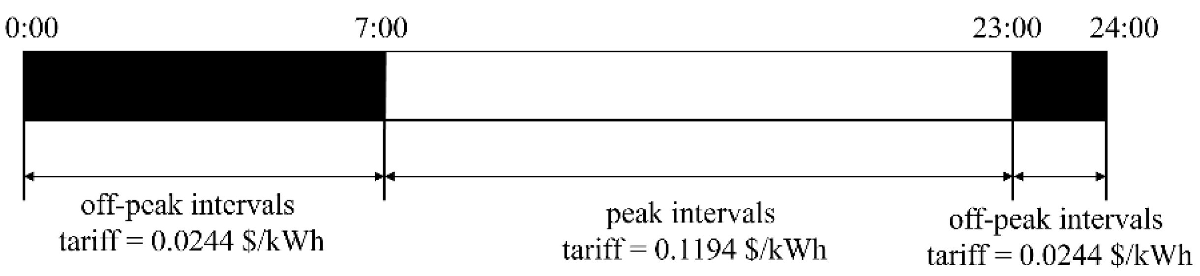
Figure 4.
The volume variation ratio of water in tanks (a) and the energy cost of pumps (b) under different penalty forms. We set , , , , , and in the experiments.
Figure 4.
The volume variation ratio of water in tanks (a) and the energy cost of pumps (b) under different penalty forms. We set , , , , , and in the experiments.

Figure 5.
Episode reward during the training with a demand of 0.3 (a), 0.6 (b), 0.9 (c).

Table 1.
Detailed settings of the agent.
| Symbol | Hyperparameter | Value |
|---|---|---|
| Structure and number of neurons in layers of the actor network | [256, 128, 64] | |
| Structure and number of neurons in layers of the critic network | [256, 128, 1] | |
| Learning rate of the actor network | ||
| Learning rate of the critic network | ||
| Maximum episode length | 24 | |
| Discounter factor | 0.9 | |
| Clip range | 0.2 | |
| Epochs | 10 | |
| Benchmark reward of energy cost | 406.54 | |
| Negative reward for the hydraulic constraint | −200 |
Table 2.
Comparison of E-PPO, PPO, and metaheuristics performance for the test cases.
| Uncertainty Parameter of Demand | Test Case | Energy Cost (USD/Day) | ||||
|---|---|---|---|---|---|---|
| GA | PSO | DE | PPO | E-PPO | ||
| 0.30 | Case 1 | 190.251 | 231.889 | 205.586 | 213.210 | 207.941 |
| Case 2 | 193.700 | 256.125 | 231.793 | 215.387 | 209.001 | |
| Case 3 | 206.623 | 283.127 | 239.610 | 218.477 | 215.993 | |
| Case 4 | 198.713 | 242.322 | 229.684 | 218.099 | 211.868 | |
| Case 5 | 190.328 | 223.991 | 212.200 | 237.575 | 215.848 | |
| 0.60 | Case 1 | 194.435 | 279.038 | 223.849 | 214.965 | 206.268 |
| Case 2 | 204.636 | 279.256 | 229.777 | 214.099 | 208.265 | |
| Case 3 | 194.163 | 255.669 | 226.321 | 229.907 | 204.839 | |
| Case 4 | 190.837 | 245.699 | 221.987 | 232.683 | 203.932 | |
| Case 5 | 200.929 | 268.320 | 224.463 | 216.151 | 209.488 | |
| 0.90 | Case 1 | 187.169 | 238.844 | 214.211 | 230.172 | 208.123 |
| Case 2 | 185.796 | 232.904 | 219.973 | 211.734 | 196.397 | |
| Case 3 | 201.102 | 259.644 | 216.285 | 209.971 | 186.099 | |
| Case 4 | 201.855 | 257.274 | 219.415 | 218.811 | 202.868 | |
| Case 5 | 217.869 | 253.887 | 238.714 | 227.810 | 220.299 | |
Table 3.
Computation time of the models.
| Uncertainty Parameter of Demand | Time (s) | ||||||
|---|---|---|---|---|---|---|---|
| GA | PSO | DE | PPO Training | E-PPO Training | PPO Application | E-PPO Application | |
| 0.3 | 1699.32 | 1291.18 | 1448.63 | 5479.30 | 5573.58 | 0.42 | 0.41 |
| 0.6 | 1640.72 | 1214.62 | 1475.45 | 5333.92 | 5407.01 | 0.44 | 0.42 |
| 0.9 | 1586.19 | 1181.03 | 1408.05 | 5833.19 | 5506.07 | 0.42 | 0.42 |
Disclaimer/Publisher’s Note: The statements, opinions and data contained in all publications are solely those of the individual author(s) and contributor(s) and not of MDPI and/or the editor(s). MDPI and/or the editor(s) disclaim responsibility for any injury to people or property resulting from any ideas, methods, instructions or products referred to in the content. |
© 2023 by the authors. Licensee MDPI, Basel, Switzerland. This article is an open access article distributed under the terms and conditions of the Creative Commons Attribution (CC BY) license (https://creativecommons.org/licenses/by/4.0/).
Share and Cite
MDPI and ACS Style
Hu, S.; Gao, J.; Zhong, D.; Wu, R.; Liu, L. Real-Time Scheduling of Pumps in Water Distribution Systems Based on Exploration-Enhanced Deep Reinforcement Learning. Systems 2023, 11, 56. https://doi.org/10.3390/systems11020056
AMA Style
Hu S, Gao J, Zhong D, Wu R, Liu L. Real-Time Scheduling of Pumps in Water Distribution Systems Based on Exploration-Enhanced Deep Reinforcement Learning. Systems. 2023; 11(2):56. https://doi.org/10.3390/systems11020056
Chicago/Turabian StyleHu, Shiyuan, Jinliang Gao, Dan Zhong, Rui Wu, and Luming Liu. 2023. "Real-Time Scheduling of Pumps in Water Distribution Systems Based on Exploration-Enhanced Deep Reinforcement Learning" Systems 11, no. 2: 56. https://doi.org/10.3390/systems11020056
Note that from the first issue of 2016, this journal uses article numbers instead of page numbers. See further details here.