Article

A Novel Large-Scale Stochastic Pushback Design Merged with a Minimum Cut Algorithm for Open Pit Mine Production Scheduling

by
Devendra Joshi
1,
Premkumar Chithaluru
1,2,*,
Aman Singh
2,3,
Arvind Yadav
1,
Dalia H. Elkamchouchi
4,
Cristina Mazas Pérez-Oleaga
3,5 and
Divya Anand
3,6
1
Department of CSE, Koneru Lakshmaiah Education Foundation (KLEF), Vaddeswaram 522302, Andhra Pradesh, India
2
Department of Project Management, Universidad Internacional Iberoamericana, Campeche 24560, Mexico
3
Higher Polytechnic School, Universidad Europea del Atlántico, C/Isabel Torres 21, 39011 Santander, Spain
4
Department of Information Technology, College of Computer and Information Sciences, Princess Nourah bint Abdulrahman University, P.O. Box 84428, Riyadh 11671, Saudi Arabia
5
Universidade Internacional do Cuanza, Estrada Nacional 250, Bairro Kaluapanda, Cuito-Bié P.O. Box 841, Angola
6
School of Computer Science and Engineering, Lovely Professional University, Phagwara 144411, Punjab, India
*
Author to whom correspondence should be addressed.
Systems 2022, 10(5), 159; https://doi.org/10.3390/systems10050159
Submission received: 5 August 2022 / Revised: 1 September 2022 / Accepted: 15 September 2022 / Published: 20 September 2022

Abstract

:
Traditional optimization of open pit mine design is a crucial component of mining endeavors and is influenced by many variables. The critical factor in optimization is the geological uncertainty, which relates to the ore grade. To deal with uncertainties related to the block economic values of mining blocks and the general problem of mine design optimization, under unknown conditions, the best ultimate pit limits and pushback designs are produced by a minimum cut algorithm. The push–relabel minimal cut algorithm provides a framework for computationally efficient representation and processing of the economic values of mining blocks under multiple scenarios. A sequential Gaussian simulation-based smoothing spline technique was created. To produce pushbacks, an efficient parameterized minimum cut algorithm is suggested. An analysis of Indian iron ore mining was performed. The developed mine scheduling algorithm was compared with the conventional algorithm, and the results show that when uncertainty is considered, the cumulative metal production is higher and there is an additional increase of about 5% in net present value. The results of this work help the mining industry to plan mines in such a way that can generate maximum profit from the deposits.

1. Introduction

Similar to other sectors, the mining sector uses production scheduling to determine the order in which mining blocks will be removed from the earth during various production periods during the life of the mine’s existence to maximize the net present value (NPV). This is a well-known linear programming with mixed integers problem that is difficult to solve when the integer variables are large. In the process referred to as conventional, first, the optimal ultimate pit, i.e., final pit contour, is defined using the Lerchs–Grossman or L-G algorithm [1,2] so that the problem size can be reduced for mine production scheduling. To optimize the mine’s annual profit while taking into account constraints such as pit slopes, the ultimate pit limit can be considered as the collection of blocks that must be removed. Selecting pit limits that maximize the gap between the overall mine value of extracted materials over the life of the mine and the total extraction cost is another way to think about maximizing the pit limits. The L-G technique applies graph theory to the problem and proves that the optimal solution to the ultimate pit problem equates to maximum graph closure. Although the purpose of the pit design decision is to reduce the size of the problem, in large mines, the reduced problem is occasionally unsolvable.
In practical scenarios, the large pit is therefore discretized into a series of small problems known as pushbacks so that mine production scheduling can be applied to those pushbacks. The generation of pushbacks is considered a long-term plan where certain constraints such as mining capacity constraints and plant capacity constraints should be respected to maximize profit from pushbacks. Pushbacks, a series of small pits, can be obtained by parameterization of the L-G algorithm [2,3]. Picard [4] demonstrated that adopting a minimal cut technique to a related graph can solve the maximum closure problem of open pit mine planning. The final pit limit and pushbacks can be created more efficiently, as shown by Hochbaum and Chen [5], who used a minimum cut/maximum flow algorithm based on Goldberg’s [6] push–relabel maximum flow/minimum cut approach. The results of Hochbaum’s [7] detailed investigation of the L-G algorithm’s theoretical complexity revealed that it is significantly more difficult than the push–relabel technique. However, these studies did not address how resource constraints are respected. In addition, the work is developed within the context of conventional optimization that does not consider uncertainty associated with different parameters; optimization is achieved assuming that all inputs are the actual values. This is a planning practice in the context of mining problems where block values are calculated from a limited sample of data and the price of metal is assumed to be constant over the mine’s life. Due to uncertainty in orebody attributes, such as grades and metal in the ground, as well as market uncertainties, such as exchange rates, it has become clear that this assumption has major limitations and may lead to unrealistic assessments and decisions [8,9]. Significant attempts have been undertaken recently to include uncertainty in mine design. To incorporate ore grade and metal uncertainty into mine planning, a set of equally likely orebody models is used in combination with stochastic optimization for the mine production scheduling problem. These efforts include the development of stochastic integer programming (SIP) models [10,11,12], intending to maximize NPV and minimize estimated deviations from production goals, as well as streamlining the use of a stochastic stockpile. Presently, the key limitation of the SIP approach is that it is computationally very demanding—an issue that is currently being addressed through research in parallelization. This is related to the work of Godoy and Dimitrakopoulos [13] and Leite and Dimitrakopoulos [14], in which scheduling is stochastically optimized using a simulated annealing algorithm. Although the optimization part of this approach is computationally very efficient, the approach requires a labor-intensive preparation of inputs, as discussed in detail by Albor and Dimitrakopoulos [12].
The mine design formulation under the stochastic scenario presented so far only takes into account geological uncertainty, assuming that the price of metal remains constant during the mine’s life. As a result, mine designs based on a fixed pricing value may fail to meet the desired goal. The typical response to this situation is really to create a new modified long-term plan and invest more funds, resulting in inefficient capital allocation, low investor returns, and a lower net present value. As a result, it is determined that including price uncertainty into production planning is required and vital, resulting in optimized production scheduling throughout the mine’s life.
To address the practical issues related to incorporating the metal price uncertainty, Meagher et al. [15] proposed a new minimal cut algorithm. Goldberg and Tarjan [16] proposed an algorithm for optimizing final pit limits that combines multiple simulated orebodies and metal price uncertainties, which generate sets of possible economic values for mining blocks. The advantage of this algorithm is that it only needs to generate a single directed graph for the minimum cut algorithm, irrespective of the number of the simulated orebodies or the sets of possible economic values of the mining blocks involved. It was shown in their paper that in a two-dimensional example, the approach can jointly handle grade/metal and market uncertainties, while other uncertainties relevant to the mining block’s economic value can also be integrated. To incorporate multiple sources of uncertainties and pushback generation, Asad and Dimitrakopoulos [17] proposed a Lagrangian relaxation-based approach with a minimum cut algorithm. In their approach, they incorporated price uncertainty by price simulation using the mean reverting price model [18]. Since the mean reverting method follows the Markov properties, the major drawback of the approach is that for calculating the conditional probability of future price value, the algorithm only considers the present value, neglecting the past value. The price value, like other time series methods, is dependent on a previous set of price values [19].
The push–relabel minimal cut algorithm is used in this paper to generate the ultimate pit and pushback while taking into account geological uncertainty. The pushbacks are generated by parameterization of the arc capacities of a minimum cut graph. A case study of an Indian iron ore deposit demonstrates the method’s complexities.

2. Literature Survey

Metals and geological uncertainties are addressed based on the number of equal probable scenario mining maps of grade, metal content, and geology using a spatial stochastic modeling approach. These techniques explicitly take into account the volumetric differences between the existing data and the assumed mining blocks and the spatial correlation among measurements from the drilling process [20,21,22]. Dimitrakopoulos and Ramazan [23] introduced the concept of ore body risk discounting, which postpones the risk for later periods by delaying the extraction period of the high-risk blocks. The main drawback of the above assumptions are they previously assigned risk probabilities for each block, discarding the grade over simulations and ignoring the uncertainty that has been jointly evaluated as groups of blocks in mining period to period [23,24].
The first mathematical models that effectively illustrated the stochastic features of OPMPS were proposed by Ramazan and Dimitrakopoulos [25]. They take into account a two-stage probabilistic model that employs multiple similar scenarios to represent uncertain geology. The decision-making process is divided into two stages: the first stage concerns the mining sequence, and the second step of each scenario addresses the production target deviation. The objective is to maximize the predicted net present value and reduce production target deviations, which decreases the chance of not fulfilling production goals. For long-term production planning in a stochastic framework, the simulated annealing concept was first presented by Godoy and Dimitrakopoulos [13] and further investigated by Leite and Dimitrakopoulos [14] and AlborConsuegra and Dimitrakopoulos [12]. This methodology was expanded to incorporate multiple mines, stockpiles, and processing destinations [26]. To maximize net present value while reducing the variation from production goals, Ramazan and Dimitrakopoulos [11] designed a stochastic integer programming model. Chatterjee and Dimitrakopoulos [27] presented a case study based on the stochastic formulation, under uncertainty. Due to this, incorporating geological uncertainty into the optimization process is more complicated but also more beneficial. These benefits were initially emphasized [11,12,13,14,28,29,30,31].

Stochastic Mine Planning under Uncertainties

Uncertainty can be measured, modeled, and quantified by geostatistical methods. This can be achieved by generating the multiple equal probability scenario of orebody realization using any geostatistical simulation method. By including uncertainty in the decision-making approach, risk can be reduced. This will allow the mine design and production planning team to generate higher profit value and a better risk management strategy. However, the mining industry is aware of the risks and uncertainties. Because stochastic models are more relevant and realistic in how they handle uncertainty and risk, they attract more attention. A common strategy for solving stochastic challenges is to evaluate the profit under various scenarios and aim to minimize production target deviations [14,28,29,30,31].
Geological uncertainty is considered to be the main reason for the unrealized forecast of cash flow by mining companies as it has a direct impact on the supply of ore and metals. The question arises of how to define the availability of ore for processing. It is not an easy question to answer, because it not only depends on the spatial distribution of the ore but also depends on the extraction sequence over time. Different extraction sequences will produce different ore supplies from the same deposit. The definition of ore is variable over time because it is a function of economic parameters and is time-dependent. The definition of available ore supply has traditionally been evaluated in the context of assumptions of fixed technical and economic constraints in time and space. In the conventional mine design and production scheduling framework, the average type of ore grade model is used in conjunction with geotechnical, economic, and environmental constraints to define the extraction order that produces the greatest economic return. The use of risk-free scenarios has shown a significant difference between forecasting economic returns and real economic returns.
Some researchers have studied the impact of geologic uncertainty on the economics of a project and used conditional simulations to conduct a risk analysis of the performance parameters of the mine plan [8,9,27,28]. They agreed that the use of smooth images or representations of geological reality (i.e., average type ore grade mode) when applying nonlinear transfer functions such as mining plans leads to unpredictable underestimation or overestimation of the performance parameters under consideration. To minimize the misclassification of resources, conditional simulation techniques are often used to estimate geological information at non-sampled locations based on stochastic model estimation techniques. This is done by interpolating data from a small number of exploration samples [27]. The stochastic framework takes multiple simulations or similarly possible grade tonnage curves by taking geological uncertainty into account, and while taking into account a single (or constant and known) grade tonnage curve, conventional techniques neglect geological uncertainty [26,29,30]. The creation of innovative scheduling systems that include simulated geological uncertainties in mine planning processes is facilitated by the existence of uncertainty modeling methods. This concept will be extended to a more general overview of the mining business when the global optimization of the mining complex is integrated. For this optimization, important factors such as hybrid demand, different processing flows, transportation systems, and product sales are included in the optimization [26]. A thorough review of long-term mine production planning with uncertainty is provided by Koushav et al. [30]. The stochastic graph closure problem of the original pushback design is a relaxed problem where the resource constraints are not included. To generate pushbacks, resource constraints have to be imposed. There are several approaches described in the literature. One strategy involves relaxing the resource constraints, putting them into the target function as a Lagrangian relaxation problem, and solving iteratively until a feasible solution is found [17]. Although the Lagrangian relaxation indeed provides a reasonable upper bound, finding a feasible solution is not assured. The convergence of the algorithm is not also guaranteed, and the algorithm is also sensitive to many parameters [32]. An alternative approach is relaxing the constraints from integer to real, solving the linear programming problem (LP-relaxation), and rounding the solution to an integer one. The limitation of the LP-relaxation algorithm is that the constraints may be violated during the rounding operation; a feasible solution is not guaranteed. It takes some postprocessing steps to reach a realistic solution. The third and most popular approach in the mining application is parameterized algorithm where the economic block value is parameterized with a multiplier λ. The parameterization algorithm of the L-G algorithm is well documented in various works of literature [2,3,33]. By scaling the economic values for all blocks using a multiplier parameter λ, a series of “nested” pits can be generated. The structure of the article is as follows: The stochastic pushback design is presented mathematically. An undiscounted graph closure formulation with geological scenarios is discussed. A discounted graph closure formulation using the minimum cut algorithm and solution approach for pushback designs are presented. A case study of an Indian iron deposit is presented, followed by conclusions.

3. Proposed Methodology

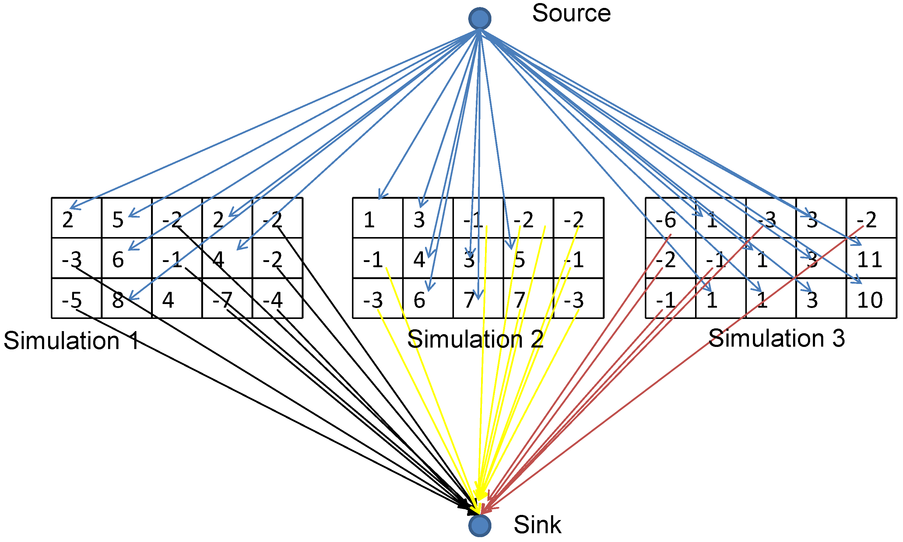
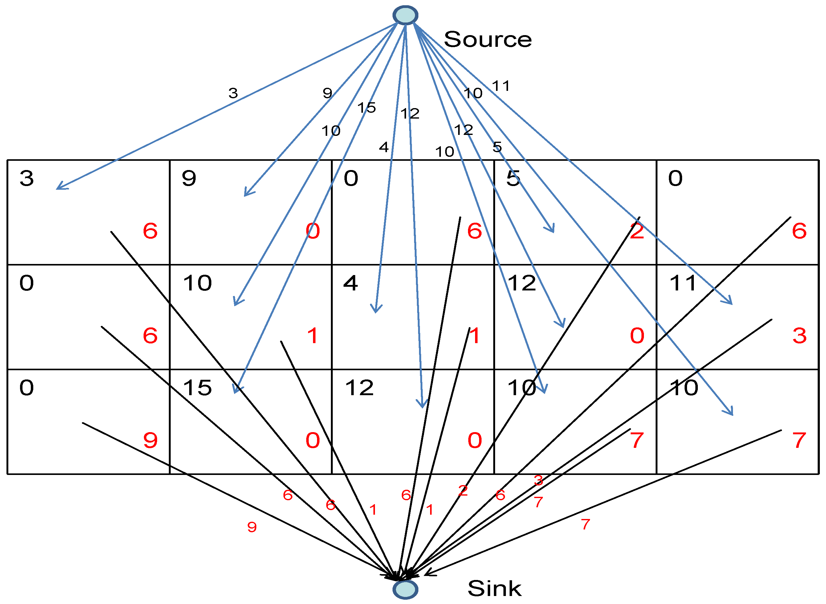
3.1. Stochastic Pushback Design Formulation

A three-dimensional block model is used to represent a mineral deposit. Each block has a set of data that describes its location in the three-dimensional model, the amount of ore or waste present, the grade, and so on. The goal of pushback design is to define the open pit mine’s contour while keeping resource limits in mind. In other words, the goal is to locate a group of blocks that can be recovered from the deposit while keeping all limits in mind to maximize profit. The problem can be defined as an ultimate pit limit problem if resource limitations are removed from the pushback design formulation. The mine pushback design challenge is presented mathematically as follows:
M a x s = 1 S t = 1 T i = 1 N c i , s , t x i , t
subject to
i = 1 N t = 1 T a i , s k x i b k s S ;   k K
x i , t τ t x j , Γ 0 , j Γ i , i N , t T
x i , t 0 , 1 , i N , t T
where Γ i is the set of blocks which have to be removed before removing block i , c i , s is the amount of revenue generated or loss incurred by removing block i from scenario s, a i , s k is the amount of kth resource generated from block i from scenario s, b k is maximum allowable kth resource constraints, and K is the total number of resource constraints.
Objective (1) is to maximize the total profit from the mine over all scenarios. Equation (2) is a set of constraints for pushback design that must be satisfied. Equation (3) is a set of slope constraints such that for extracting block i from a deposit, all blocks in a set Γ i   have to be extracted. Equation (4) ensures that a block is either extracted or remains in the deposit.
The c i , s of the individual blocks is calculated as follows:
c i , s = T i × g i × R E C × p s SC M C P C ,   if   T × G i × R E C × p s S > P C M C , otherwise
where M C is mining cost, P C is processing cost, T i is block i tonnage, g i is block i grade, R E C   is recovery, p s is price simulation scenario, and S C is selling cost.
It is clear from the above formulation of both single scenarios and multiple scenarios that pushback design is an NP-hard problem. However, if the constraints of Equations (2) and (3) are eliminated from these problems, they are efficiently solvable by any graph closure algorithm. In this paper, a push–relabel minimum cut approach is used for solving the graph closure problem and then a parameterized approach is applied to impose resource constraints for pushback design.

3.1.1. Stochastic Graph Closure with Multiple Scenarios

A minimum graph cut issue can be used to model pushback design without resource limitations. Using Equation (5), the block economic value ( c i , s ) is determined. Blocks with positive values ( c i , s > 0 ) are ore blocks, while those with negative or zero values ( c i , s 0 ) are waste blocks. The directed graph is considered to have nodes at each block. Two special nodes are present: a source (s) and a sink (t). All nodes identified as ore blocks are linked to the source node, and the economic values of those blocks are represented by the capacity of those arcs ( c i , s ). However, all nodes in the model that are labeled as waste blocks are linked to the sink node, and the capacities are equal to the absolute value of the waste blocks’ economic values ( c i , s ).
A group of underlying blocks must first be extracted to mine a specific block, i. The slope constraints stated in Equation (3) can be maintained to achieve this. While removing the target block, it is necessary to determine the underlying blocks that must be removed to meet slope constraints. As a result, arcs are drawn from block i to the overlying blocks that have capacities of infinity ( ). Because slope constraint arcs have an infinite value, they will never be included in the minimum cut.
After forming the directed graph using multiple models as shown in Figure 1, the minimum cut algorithm can be implemented to solve pushback design without resource constraints. If the minimum cut algorithm is implemented with the above-described directed graph with S number of scenarios, It is not guaranteed that the same block will fall on the same side of the minimum cut in all scenarios. However, the decision should be binary (1, 0); i.e., a block is either within the closure or outside the closure, regardless of the number of scenarios. In the graph, an additional constraint is required to ensure that a provided block falls on the identical side of the cut in all scenarios. This constraint can be implemented by placing bidirectional arcs with infinite capacity ( ) among the same block i from different scenarios. Since these bidirectional arcs have infinite capacity, they will never be in the minimum cut, which ensures that there will be no such situation when the same block from different scenarios will fall on different sides of the minimum cut. Therefore, the pit generated by the minimum cut algorithm with multiple scenarios of orebody models is a valid pit where all constraints are respected except resource constraints. These nodes can be combined into a single node because the identical block from the many scenarios will fall on the same side of the minimal cut. It is possible to combine the arcs from the source node to the merging nodes from various scenarios into a single arc, and the capacity of the resulting arc will be s = 1 S c i , s   if c i , s > 0 . Similarly, a single arc can be formed from a merge to the sink node(t), and the capacity of the arc will be s = 1 S c i , s if c i , s 0 .
This concept is presented in Figure 2, where the graph is developed by merging the three scenarios of orebody models from Figure 1. In this figure, each block is assigned two values. The top-left corner value is the sum of the economic values of a block over all scenarios if c i , s > 0 . The bottom-right corner value is the sum of the absolute block economic value over all scenarios if c i , s 0 . The value in the top-right corner represents the arc capacity from the source to that node, and the value in the bottom-left corner represents the arc capacity from that node to the sink. For example, the top-left block in Figure 2 has an arc capacity from the source node to the node of 3, which is a sum of 2 and 1—the block economic values of scenario 1 and scenario 2, respectively. The same node has a connection to the sink with a capacity of 6, the absolute block value in simulation 3.
To generate pushbacks, an iterative parameterization algorithm is applied until resource constraints are respected. The authors have applied a parameterized approach and proposed an approach to update the λ value in iteration.
After applying the parameterization of the block economic values, the problem can be rewritten as
Φ λ = m a x t = 1 T i = 1 N λ s = 1 S d t i , s x i , t
x i , t τ t x j , Γ 0 , j Γ i , i N
x i 0 , 1 , i N , and t = 1 T x i , t 1
where
λ = λ   if   s = 1 S d t i , s > 0 = 1                     o t h e r w i s e
A parameterization factor has a bound within the λ multiplier (0, 1). When λ is equal to 1, the problem is solved using the objective function Equations (6) and (9) without the need for pushback constraints. The goal of the parameterization strategy is to choose an appropriate λ value that will enable the problem posed in Section 3 to have a large upper-bound solution. The minimum cut algorithm covered in Section 3.1.1 can be used to solve the objective function of Equation (6) for a particular value of λ .
Pushbacks are significantly influenced by the parameter λ , which is a multiplier of the directed arc capacity. The random selection of λ might lead to pushbacks with wide gaps, which would be unfavorable for mining. Any minimum cut algorithm can be used to maximize the optimization problem for a specific λ value once the merged graph has been constructed. The achieved solution, however, will ignore pushbacks’ resource limitations. An iterative technique was used to choose the λ value to satisfy two resource limitations. The process begins with λ = 0 and progresses through the update of the λ value by λ + λ as far as resource constraints are satisfied for all scenarios S .
To generate pushbacks, the following pseudo-code is used:
1.
Set a parameter λ such that 0 < λ < 1.
2.
Start λ = 0.
3.
Assign best productionks = 0 at λ = 0 for all resource limitations k and scenario s .
4.
Increase λ by a small value ∆λ, i.e., λ = λ + Δ λ
5.
Solve Φ λ .
6.
If ( b e s t   p r o d u c t i o n k s b k , s , k ) from a solution of Φ λ ,
Update λ value by Δ λ   i . e . ,   λ = λ + Δ λ ;
best productionks = i = 1 N a k i , s x i .
7.
Go to step 5.
8.
End.
Thus, both for resolution and computational efficiency, selecting the step size ∇λ is crucial. If ∇λ has been chosen too small, the algorithm will take a long time to converge. On the other hand, if the ∇λ value has been chosen too high, a large gap may be observed between the two pushbacks. Therefore, instead of choosing a fixed ∇λ value, a ∇λ value is updated in each iteration depending on how far away from the convergence point the solution is. By choosing a monotonically decreasing function for variable ∇λ, the large step size can be selected when the algorithm is far from the convergence point, and the small step size can be selected when the algorithm is approaching the convergence point. Equation (10) is used for calculating the value of ∇λ.
λ = k = 1 K s = 1 S w i , s b k i = 1 N a i , s k ε
where w i , s are weights associated with kth resource constraints for grade scenario s and ε is a small constant number. Since the values of bk are constant and the values of best productionks are increased after each iteration, Equation (10) ensures that λ value will have a monotonically decreasing function. When the algorithm of the pseudo-code is close to violating the resource constraints, the λ value will be incremented by a small magnitude.

4. Results and Discussion

Composited iron sample analyses were statistically examined. Table 1 displays the statistical analysis for the composited data. The iron grade is skewed towards the right, although with relatively less variance, as the table demonstrates. The frequency distribution of the dataset was also prepared using the histogram plot (Figure 3). It clearly shows the skewness property of the dataset.
The grade was estimated using ordinary kriging [34]. The variogram analysis was used to determine the data’s spatial correlation [35]. For testing the anisotropy, both directional and omnidirectional variograms were examined. The variogram analysis of the deposit was exceptionally complicated in a proposed mine study due to the presence of many different lithotypes. Seven different lithotypes are present in this mine. The modeling of the deposit without classifying lithology may lead to a large error in estimation. Some of the lithotypes show very less variance compared to the others as well as compared to the original data. A better variogram model may be obtained for some of the lithotypes by modeling each lithology separately. Both approaches were used to estimate the deposit. First, without considering lithology, an omnidirectional variogram for iron was constructed. A spherical variogram model was fitted for modeling spatial continuity. The range, sill, and nugget of the variable are 255.28, 31.26, and 38.08, respectively. After fitting the variograms, the search for anisotropy was carried out.
The variograms were calculated in eight different directions with 22.5° tolerance. The directional variogram demonstrated that the deposit has directional anisotropy with a major axis along the N–S direction. The major to semi-major and major to minor ratios are 3:1 and 5:1, respectively. In the second approach, an attempt was made to develop a separate variogram for each lithotype. Unfortunately, it was not possible to obtain an experimental variogram due to a smaller number of available data for individual lithology. Therefore, it was decided to perform resource evaluation with composited data without considering lithology in this study mine.
The block model of the deposit was estimated using the ordinary kriging technique. Because of the size of the selective mining unit (SMU), the estimated block size is 20 m × 20 m × 10 m [36]. A total number of 14 benches is considered for this deposit. Figure 4 depicts the iron ore grade map of one of the fourteen benches. Following that, the estimated block model was used as input for mine production scheduling.
The proposed models were implemented in a MATLAB platform and solved with the CPLEX solver [37]. Table 2 presents the specific economic parameters that were utilized in this study. The final result is presented in Table 3 and Table 4 for the traditional model and Table 5 and Table 6 for the proposed model. Figure 5 depicts the production schedule of the proposed model.
A period-wise production schedule is shown in Table 3 and Table 5. Ore production (million tons), metal production (kilotons), and NPV (USD 1 million) generated by the traditional and proposed model are calculated in Table 4 and Table 6. It was found that when these two models were compared, they produced different amounts of ore, waste, and metal content over the length of the mine’s life. However, the proposed model generates comparatively more NPV than the traditional model because of the different extraction sequence. Due to the production of more ore and metal in a shorter amount of time and the consequent generation of greater discounted cash flow as compared to the traditional model, the suggested model’s NPV is determined to be higher. The traditional approach requires less calculation time than the suggested model; due to the increase in the number of constraints and decision factors, this is quite obvious. Additionally, the proposed model is more reliable for efficient production scheduling over the mine’s life. The mining sector is looking for more advanced solutions to address the challenges of large-scale production scheduling in many unpredictably occurring scenarios. Mine planners typically employ optimization strategies that produce the highest undiscounted profits. Different companies of mining software are becoming aware of the drawbacks of conventional mine planning methods and the necessity of including uncertainty in the mine plan. The findings of this case study demonstrate how incorporating uncertain parameters enables mine planners to better understand the risk associated with not attaining targets and the efficacy of their cash flow analysis. Mine planners have excellent potential to maximize returns on their investment with a high degree of confidence and a shorter mine life by using these optimization techniques.

5. Conclusions and Future Scope

In this paper, an uncertainty-based ultimate pit limit and pushback design algorithm was developed using a graph cut algorithm to integrate geological-based models. The suggested approach demonstrates that it is comparatively easy to create a minimum cut network flow model that incorporates uncertainty, and it can deal with uncertainty in the block economic value of the mining blocks being sequenced. Different scenarios from various production periods were merged with the stochastic framework as opposed to traditional pit optimization, which only considered one constant grade value for the life of the mine. The smoothing spline model was used to estimate trends, and a sequential Gaussian simulation approach was used to simulate the residual values. The directed graph was constructed using a simulated grade, and pushbacks were generated by parameterizing the directed graph. The key benefit of the suggested technique is that it is computationally very quick, making it possible for large-scale deposits to integrate grade uncertainties in the optimization process. The proposed method was applied to an Indian iron ore deposit. Results show that a total number of nine nearly equal size pushbacks were generated. When compared with a traditional model, it was observed that the proposed stochastic optimization algorithm generates 5% more NPV. It is anticipated that the applicability and clarity of the solution structure given in this research would make it simpler for the mining industry to incorporate. However, there are still vital areas for future study that need to be investigated further. First, while grade-related uncertainty is taken into account in our models, the actual range of uncertainty is far wider and displays itself in a variety of ways, most significantly in the economical or operational constraints. Therefore, it is expected that including market uncertainty inside the suggested framework will be beneficial—given that doing so can be done without falling into “computational complexity”.

Author Contributions

Conceptualization, D.J., P.C. and A.Y.; methodology, D.J., P.C. and A.S.; software, D.J., P.C. and D.H.E.; validation, D.J., P.C. and C.M.P.-O.; analysis, D.J., P.C. and A.S.; investigation, D.A.; resources, A.S. and D.H.E.; writing—original draft preparation, D.J. and P.C.; writing—review and editing, D.J., P.C., A.S. and A.Y.; supervision, A.S. and D.A.; project administration, C.M.P.-O.; All authors have read and agreed to the published version of the manuscript.

Funding

The research was funded by Princess Nourah bint Abdulrahman University Researchers Supporting Project number (PNURSP2022R238), Princess Nourah bint Abdulrahman University, Riyadh, Saudi Arabia.

Data Availability Statement

After a non-disclosure agreement was signed, the data utilized in the study were obtained from a mining company. As a result, the data from the resource model cannot be shared. The solutions, however, can be shared. Please contact the primary author for clarification.

Acknowledgments

The authors acknowledge Princess Nourah bint Abdulrahman University Researchers Supporting Project number (PNURSP2022R238), Princess Nourah bint Abdulrahman University, Riyadh, Saudi Arabia, and the support of NIT Rourkela and the mining industry, who provided the environment and data to carry out the case study of this paper.

Conflicts of Interest

The authors declare no conflict of interest.

References

  1. Lerchs, H.; Grossmann, I.F. Optimum Design of Open Pit Mines. Canad. Inst. Mining Bull. 1965, 58, 47–54. [Google Scholar]
  2. Whittle, J.A. Decade of open-pit mine planning and optimization—The craft of turning algorithms into packages. In Proceedings of the APCOM ‘99 (Golden: Colorado School of Mines), Golden, CO, USA, 20–22 October 1999; pp. 15–24. [Google Scholar]
  3. Bongarcon, F.D.M.; Guibal, D. Parameterization of Optimal Designs of an Open Pit Beginning of a New Phase of Research. AIME Trans. 1983, 274, 1801–1805. [Google Scholar]
  4. Picard, J.C. Maximal closure of a graph and applications to combinatorial problems. Manag. Sci. 1976, 22, 1268–1272. [Google Scholar] [CrossRef]
  5. Hochbaum, D.S.; Chan, A. Performance analysis and best implementations of old and new algorithms for the open-pit mining problem. Oper. Res. 2000, 48, 894–914. [Google Scholar] [CrossRef]
  6. Goldberg, A.V. The Partial Augment–Relabel Algorithm for the Maximum Flow Problem. In Proceedings of the 16th Annual European Symposium Algorithms, Karlsruhe, Germany, 15–17 September 2008; pp. 466–477. [Google Scholar]
  7. Hochbaum, D.S. A new-old algorithm for minimum cut in closure graphs. Networks 2001, 34, 171–193. [Google Scholar] [CrossRef]
  8. Dimitrakopoulos, R.; Farrelly, C.T.; Godoy, M. Moving forward from traditional optimization: Grade uncertainty and risk effects in open pit design. Trans. Instn. Min. Metall. (Sec. A Min. Technol.) 2002, 111, A82–A88. [Google Scholar] [CrossRef]
  9. Dimitrakopoulos, R.; Abdel-Sabour, S.A. Evaluating mine plans under uncertainty: Can the real options make a difference? Res. Policy 2007, 32, 116–125. [Google Scholar] [CrossRef]
  10. Ramazan, S.; Dimitrakopoulos, R. Stochastic optimization of long-term production scheduling for open pit mines with a new integer programming formulation. In, Orebody modelling and strategic mine planning: Uncertainty and risk management models. AusIMM Spectr. Ser. 2007, 14, 385–392. [Google Scholar]
  11. Ramazan, S.; Dimitrakopoulos, R. Production Scheduling with Uncertain Supply: A New Solution to the Open Pit Mining Problem. Opt. Eng. 2013, 14, 361–380. [Google Scholar] [CrossRef]
  12. Albor, F.; Dimitrakopoulos, R. Algorithmic Approach to Pushback Design Based on Stochastic Programming: Method, Application, and Comparisons. IMM Trans. Sect. A Min. Technol. 2010, 119, 88–101. [Google Scholar]
  13. Godoy, M.; Dimitrakopoulos, R. Managing risk and waste mining in long-term production scheduling of open-pit mines. SME Trans. 2004, 316, 43–50. [Google Scholar]
  14. Leite, A.; Dimitrakopoulos, R. A stochastic optimization model for open pit mine planning: Application and risk analysis at a copper deposit. IMM Trans. Min. Technol. 2007, 116, 109–118. [Google Scholar] [CrossRef]
  15. Meagher, C.; Sabour, S.; Dimitrakopoulos, R. Pushback design of open pit optimization under geological and market uncertainties. Int. Symp. Orebody Modeling Strateg. Mine Plan. Old New Dimens. A Chang. World Perth Aust. 2009, 17, 291–298. [Google Scholar]
  16. Goldberg, A.V.; Tarjan, R.E. A new approach to the maximum flow problem. J. ACM 1998, 35, 921–940. [Google Scholar] [CrossRef]
  17. Asad, M.W.A.; Dimitrakopoulos, R. Implementing a parametric maximum flow algorithm for optimal open pit mine design under uncertain supply and demand. J. Oper. Res. Soc. 2013, 64, 185–197. [Google Scholar] [CrossRef]
  18. Schwartz, E.S. The stochastic behavior of commodity prices: Implications for valuation and hedging. J. Financ. 1997, 52, 923–973. [Google Scholar] [CrossRef]
  19. Azadeh, A.; Moghaddam, M.; Khahzad, M.; Ebrahimipour, V. A flexible neural network-fuzzy mathematical programming algorithm for improvement of oil price estimation and forecasting. Comput. Ind. Eng. 2012, 62, 421–430. [Google Scholar] [CrossRef]
  20. Godoy, M. The Effective Management of Geological Risk. Ph.D. Thesis, University of Queensland, St Lucia, Australia, 2003. [Google Scholar]
  21. Goovaerts, P. Geostatistics for Natural Resources Evaluation; Applied Geostatistics Series; Oxford University Press: New York, NY, USA, 1997. [Google Scholar]
  22. Remy, N.; Boucher, A.; WU, P. Applied Geostatistics with Sgems—A User’s Guide; Cambridge University Press: Cambridge, UK, 2009. [Google Scholar]
  23. Dimitrakopoulos, R.; Ramazan, S. Uncertainty-based production scheduling in open pit mining. SME Trans. 2004, 316, 106–116. [Google Scholar]
  24. Dimitrakopoulos, R.G.; Grieco, N. Stope design and geological uncertainty: Quantification of risk in conventional designs and a probabilistic alternative. J. Min. Sci. 2009, 45, 152–163. [Google Scholar] [CrossRef]
  25. Ramazan, S.; Dimitrakopoulos, R. Stochastic Optimisation of Long-Term Production Scheduling for Open Pit Mines with a New Integer Programming Formulation. Adv. Appl. Strateg. Mine Plan. 2018. [Google Scholar] [CrossRef]
  26. Goodfellow, R.; Dimitrakopoulos, R.G. Simultaneous Stochastic Optimization of Mining Complexes and Mineral Value Chains. Math. Geosci. 2017, 49, 341–360. [Google Scholar] [CrossRef] [PubMed]
  27. Chatterjee, S.; Dimitrakopoulos, R. Production scheduling under uncertainty of an open-pit mine using Lagrangian relaxation and branch-and-cut algorithm. Int. J. Min. Reclam. Environ. 2020, 34, 343–361. [Google Scholar] [CrossRef]
  28. Joshi, D.; Paithankar, A.; Chatterjee, S.; Equeenuddin, S.M. Integrated Parametric Graph Closure, and Branch-and-Cut Algorithm for Open Pit Mine Scheduling under Uncertainty. Mining 2022, 2, 32–51. [Google Scholar] [CrossRef]
  29. Moreno, E.; Emery, X.; Goycoolea, M.; Morales, N.; Gonzalo, N. A two-stage stochastic model for open pit mine planning under geological uncertainty. In Proceedings of the 38th International Symposium on the Application of Computers and Operations Research in the Mineral Industry (APCOM 2017), Golden, CO, USA, 9–11 August 2017. [Google Scholar]
  30. Koushavand, B.; Askari-Nasab, H.; Deutsch, C.V. A linear programming model for long-term mine planning in the presence of grade uncertainty and a stockpile. Int. J. Min. Sci. Technol. 2014, 24, 451–459. [Google Scholar] [CrossRef]
  31. Joshi, D.; Satpathy, S.K. Production scheduling of open pit mine using sequential branch-and-cut and longest path algorithm: An application from an African copper mine. J. Eur. Syst. Autom. 2020, 53, 629–636. [Google Scholar] [CrossRef]
  32. Tachefine, B.; Soumis, F. Maximal Closure on a Graph with Resource Constraints. Com. Oper. Res. 1997, 24, 981–990. [Google Scholar] [CrossRef]
  33. Seymour, F. Pit limit parameterization from modified 3D Lerchs-Grossmann Algorithm. SME Trans. 1995, 298, 1860–1864. [Google Scholar]
  34. Coburn, T.C. Geostatistics for Natural Resources Evaluation. Technometrics 2000, 42, 437–438. [Google Scholar] [CrossRef]
  35. Deutsch, C.V.; Journel, A.G. GSLIB: Geostatistical Software Library and User’s Guide; Oxford University Press: New York, NY, USA, 1998. [Google Scholar]
  36. Hustrulid, W.A.; Kuchta, M. Open Pit Mine Planning and Design, Two Volume Set, 2nd ed.; Taylor & Francis: Leiden, The Netherlands, 2006. [Google Scholar]
  37. ILOG. CPLEX 12.5 User’s Manual; IBM: Armonk, NY, USA, 2012. [Google Scholar]
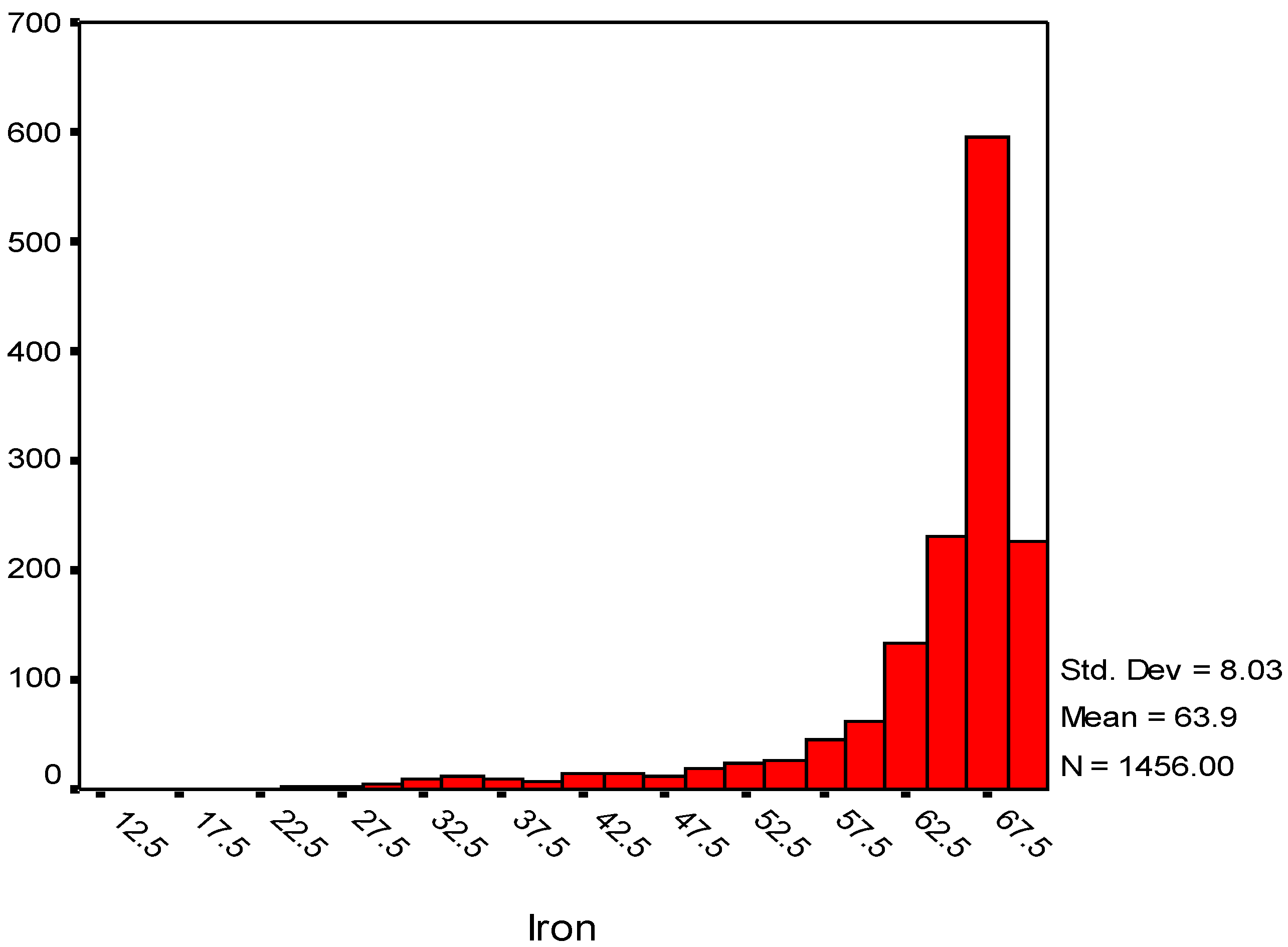
Figure 1. Graph constructed from multiple scenarios of models.
Systems 10 00159 g001
Figure 2. Graph constructions after merging three block economic models generated using multiple scenarios.
Systems 10 00159 g002
Figure 3. Histogram plot of composited data.
Systems 10 00159 g003
Figure 4. Map showing the ore grade for one of the deposit’s fourteen benches.
Systems 10 00159 g004
Figure 5. Production schedule of the proposed model year wise.
Systems 10 00159 g005
Table 1. Composited iron ore descriptive statistics.
StatisticsSample No.Mean
(%)
Variance
(%2)
Coefficient of
Variation
SkewnessKurtosis
Iron145663.8564.5212.58−2.748.39
Table 2. Specific details on the values of certain parameters.
Description Value
Slope angle (degree)45°
Block dimensions (m × m × m)20 × 20 × 10
Recovery (%)0.9
Cutoff grade of iron (%)55.26
Discount cash flow (%) 0.10
Iron selling price (USD/ton) 40
Iron ore selling cost (USD/ton) 3.6
Iron ore processing cost (USD/ton) 12
Iron ore mining cost (USD/ton) 3
Table 3. Traditional model block extraction year-wise.
Year (T)No. of Blocks (N)No. of Blocks Extracted per YearSolution Time
in Seconds (t)
Gap (%)No. of Scenarios (s)
116,532876157.120.011
215,656181537.190.001
313,8411620151.040.001
412,2211919263.660.011
510,3022172129.850.001
68130214262.790.011
7598818678.940.001
8412115869.280.001
9253512682.790.001
10126712670.360.001
Total 823.02 s
Table 4. Traditional model of calculated ore, waste, metal, and NPV per year.
YearOre (Mt)Waste (Mt)Metal (Kt)NPV (USD 1 Million)
17,170,0002,850,00050,000101,000,000
28,000,00012,800,00040,40056,900,000
38,000,00010,500,00036,70043,900,000
48,000,00014,000,00036,90038,800,000
58,000,00016,900,00038,80038,100,000
68,000,00016,500,00039,60036,200,000
78,000,00013,400,00038,30031,800,000
88,000,00010,100,00035,90026,100,000
98,000,0006,510,00032,20019,600,000
107,700,0006,800,00027,50012,700,000
Total7.88 × 1071.10 × 1083.76 × 1054.05 × 108
Table 5. Proposed model block extraction year-wise.
Year (T)No. of Blocks (N)No. of Blocks Extracted per YearSolution Time
in Seconds (t)
Gap (%)No. of the Scenarios (s)
116,532917351.490.2320
215,6151925577.380.5820
313,6901616233.551.4620
412,07418671309.132.7920
510,2072112589.092.7620
680952185111.982.4320
75910216722.360.0520
83743175015.371.7720
9199314643.460.8820
10529LeftNo solution or infeasible sol.
Total 3213.81
s
Table 6. Proposed model of average calculated ore, waste, metal, and NPV per year.
YearOre (Mt)Waste (Mt)Metal (Kt)NPV (USD 1 Million)
17,114,50033,755,0049,16098,380,000
27,738,00014,280,00041,70561,000,000
37,816,00010,670,00038,84049,795,000
47,709,00013,650,00037,66041,975,000
57,755,50016,425,00039,34540,275,000
67,643,00017,355,00040,35538,535,000
77,776,50017,020,00041,57536,690,000
87,717,50012,305,00037,29528,465,000
97,629,0009,117,50032,53020,465,000
Sum6.89 × 1071.14 × 1083.58 × 1054.16 × 108
Publisher’s Note: MDPI stays neutral with regard to jurisdictional claims in published maps and institutional affiliations.

