
Multi-Objective Sustainable Closed-Loop Supply Chain Network Design Considering Multiple Products with Different Quality Levels


 ,
,  ,
,  ,
,  and
and
Abstract
:1. Introduction
- Designing a robust multi-objective mathematical programming model for a sustainable closed-loop supply chain that can integrate the design of forward and reverse networks (horizontal integration) and optimize strategic and tactical decisions simultaneously (vertical integration). It should be mentioned that the strategic decisions are mainly related to the structure of the supply chain in the upcoming years; how the supply chain is configured, how resources are allocated, and what processes take place at each level of the supply chain. Strategic decisions in this study are to determine the location of facilities such as factories, distribution centers, and collection centers (long-term decisions). The tactical decisions deal with satisfying demands, binding contracts, inventory management and control policies, and so on. In the planning phase, organizations need to consider demand uncertainty within the planning time horizon. Therefore, in this research, it is determined how many products should be sent to each warehouse and which warehouses should satisfy the demand of which market segment under uncertainty conditions.
- Considering several products with various quality levels (green/non-green) for different types of customers with different consumption trends.
- Taking the uncertainty of supply chain parameters such as cost and demand into account. Nowadays, costs are swiftly increasing, leading to changes in customer demands. This fact must be considered in decision-making so that more reliable and accurate decisions can be made.
2. Literature Review
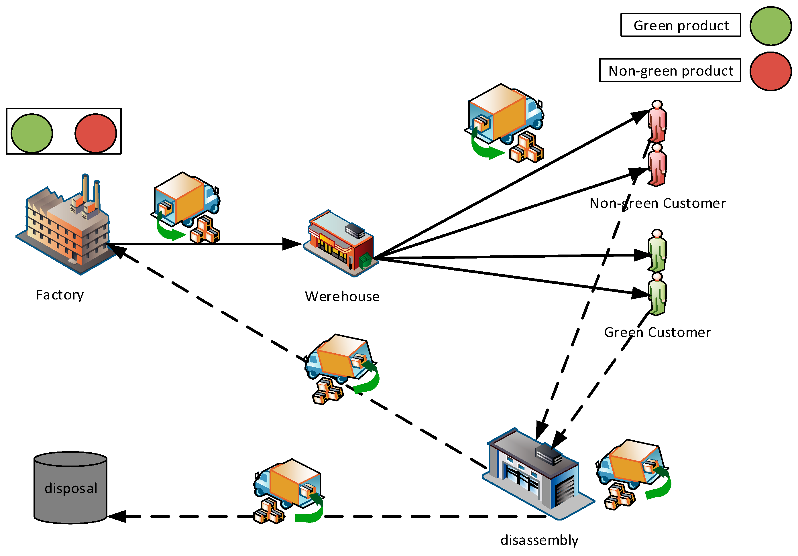
3. Problem Statement and the Mathematical Programming Model
- New goods, whether brand new or remanufactured, are transported to the forward path of the network (factory to warehouse and warehouse to customer) to meet the customer’s demand.
- The products to be disposed of are collected from the customers and sent to the DCs for the disassembly process. In the disassembly centers, if the product is reconstructed, then it will enter the production cycle, and if it is non-recyclable, it is sent to disposal centers.
- The disassembled product is delivered from the DCs to the factory for the reproduction process.
- Factories have two production processes. One is the assembly of products sent from DCs and another is the supply of raw materials from suppliers and manufacturing of new products.
- The demands of all customers are defined as fuzzy numbers.
- All products that are produced in a factory and stored in the warehouse are always free of defects.
- All customer demands are supplied by factories or through warehouses.
- All disposed of products that are entered into DCs will be recovered with a specified probability of θ and disposed of with a probability of 1-θ.
- The fixed and variable costs of constructing supply chain institutions are pre-determined and fuzzy in nature.
- The model is examined in the multi-product mode with green and non-green quality levels.
- The customers are divided into two categories of green customers and non-green customers according to their attitude towards product consumption (green/non-green) and their demands for green and non-green products are analyzed under uncertainty conditions (green products are products made of environmentally friendly material).
- Products can be produced in both green and non-green modes according to the customers’ demands.
| Sets | |
| P | Products index |
| Q | Products quality level index (green/non-green) |
| F | Potential factories index |
| W | Potential warehouses index |
| C | Customers’ index |
| I | Index of potential DCs |
| N | Potential centers index |
| TF | Transportation options for factories |
| TW | Transportation options for warehouses |
| TK | Transportation options for customers |
| TN | Transportation options for disposal centers |
| Parameters | |
| The demand for product with quality level for customer c | |
| The transfer cost per unit from factory f to warehouse with transportation mode | |
| The transfer cost per unit from warehouse with transportation mode to customer c | |
| The transfer cost per unit from customer with transportation mode to collection/disassembly site | |
| The transfer cost per unit from disassembly center with transportation mode to the factory site | |
| The transfer cost per unit from disassembly center with transportation mode tn to landfill | |
| The transportation rate from factory to warehouse w with transportation mode tf | |
| The transportation rate from warehouse w with transportation mode to customer | |
| The transportation rate from customer with transportation mode to collection/disassembly site | |
| The transportation rate from disassembly center with transportation mode ti to factory site | |
| The transportation rate from disassembly center with transportation mode to landfill | |
| The variable cost per producing unit of product p with quality level in factory | |
| The variable cost per maintaining unit of product in the warehouse w | |
| The variable cost per collecting unit of product from customer c for the recovery operation | |
| The variable cost per disassembling a unit of product p with quality level at the DC site | |
| The variable cost per reproduction of a unit of product p with quality level q assembled at factory | |
| The maximum production capacity of product p with quality level in factory | |
| The maximum capacity for the reproduction of product p with quality level q in factory | |
| The minimum percentage of product with quality level that is collected for recycling from the customer. | |
| A percentage of products that are shipped intactly from the DC to the factory. | |
| The distance from factory f to warehouse | |
| The distance from warehouse to customer | |
| The distance from customer c to collection/DC site | |
| The distance of DC from factory site f | |
| The transportation rate from DC to landfill | |
| Environmental Parameters | |
| The CO2 emission rate per manufacturing of a unit product with quality level q in factory | |
| The emission rate of CO2 per production of a unit product with quality level q in factory | |
| The CO2 emission rate per processing of a unit product p with quality level in warehouse | |
| The emission rate of CO2 per recovery of a unit product p with quality level q in DC | |
| The CO2 emission rate per reproduction of a unit product p with quality level q in factory | |
| The emission rate of CO2 with transportation mode tf to transfer a unit product p from factory to warehouse in unit of length | |
| The CO2 emission rate corresponding with transportation mode tw to transfer a unit product from the warehouse to the customer in unit of length | |
| The emission rate of CO2 with transportation mode tk to collect a unit product from customer to DC in unit of length | |
| The CO2 emission rate corresponding with transportation mode to transfer a unit product from DC to factory in unit of length | |
| The fixed cost of constructing factory | |
| The fixed cost of constructing the warehouse | |
| The fixed cost of constructing DC site | |
| The maximum processing capacity in the warehouse | |
| The maximum capacity for recovery operation in DC | |
| The maximum capacity to dispose of products in | |
| is equal to one if factory is open and otherwise equal to zero | |
| is equal to one if warehouse w is open, otherwise equal to zero | |
| is equal to one if DC is open, otherwise equal to zero |
| The number of -type products with quality level that are transferred from factory to warehouse with transportation option | |
| The number of p-type products with quality level that are transferred from the warehouse and the customer with transportation option | |
| The number of -type products with quality level sent from customer to the DC site with transportation option for recycling | |
| The number of products p with quality level that are passed transferred from the DC to the disposal site n with transportation option for disposal | |
| The amount of product that is sent from DC to factory with transportation option | |
| The amount of product with the new quality level that should be produced in factory |
3.1. Robust Possibilistic Programming Model
3.2. The Proposed Robust Model for the Sustainable Closed-Loop Supply Chain Problem
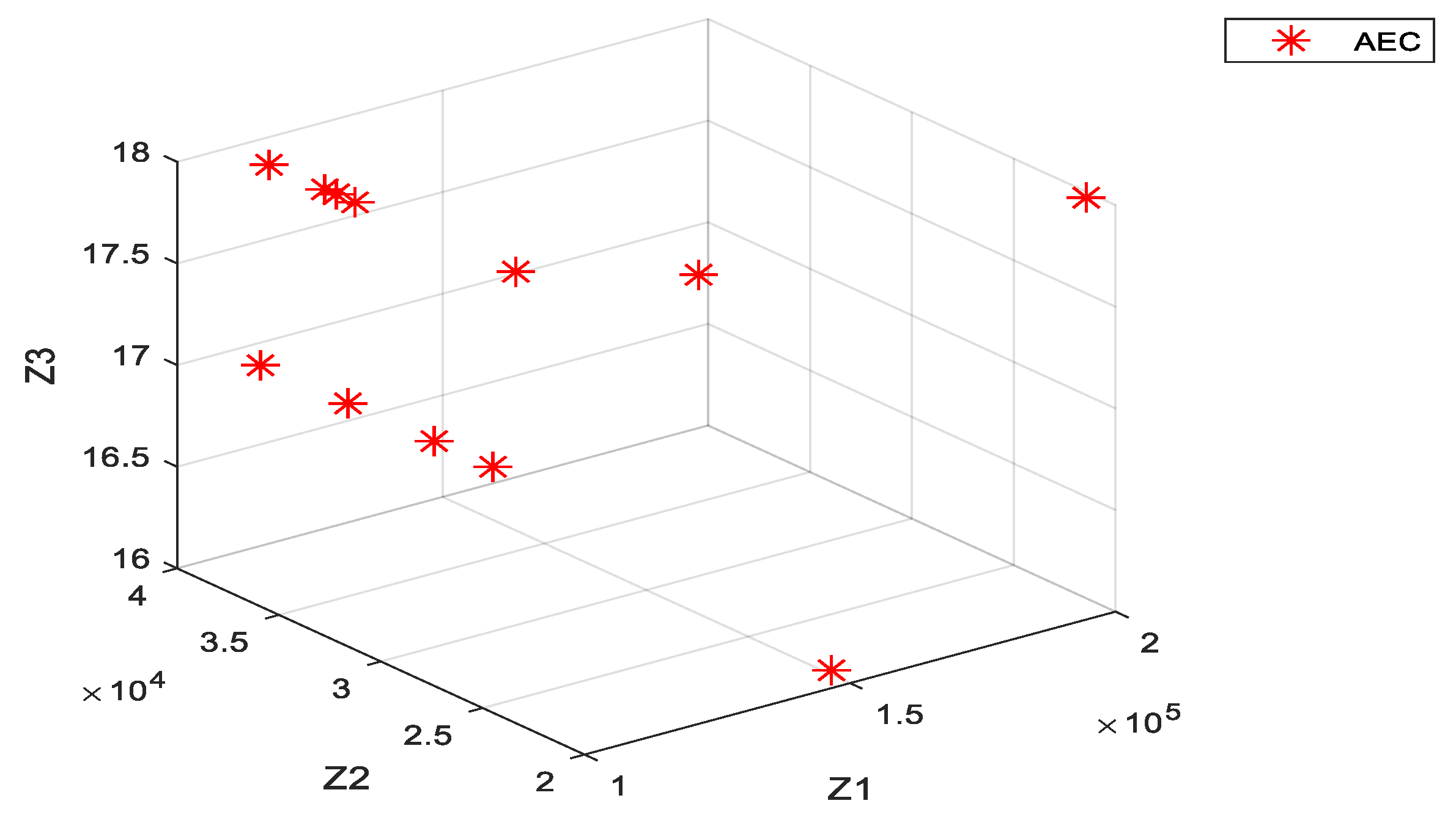
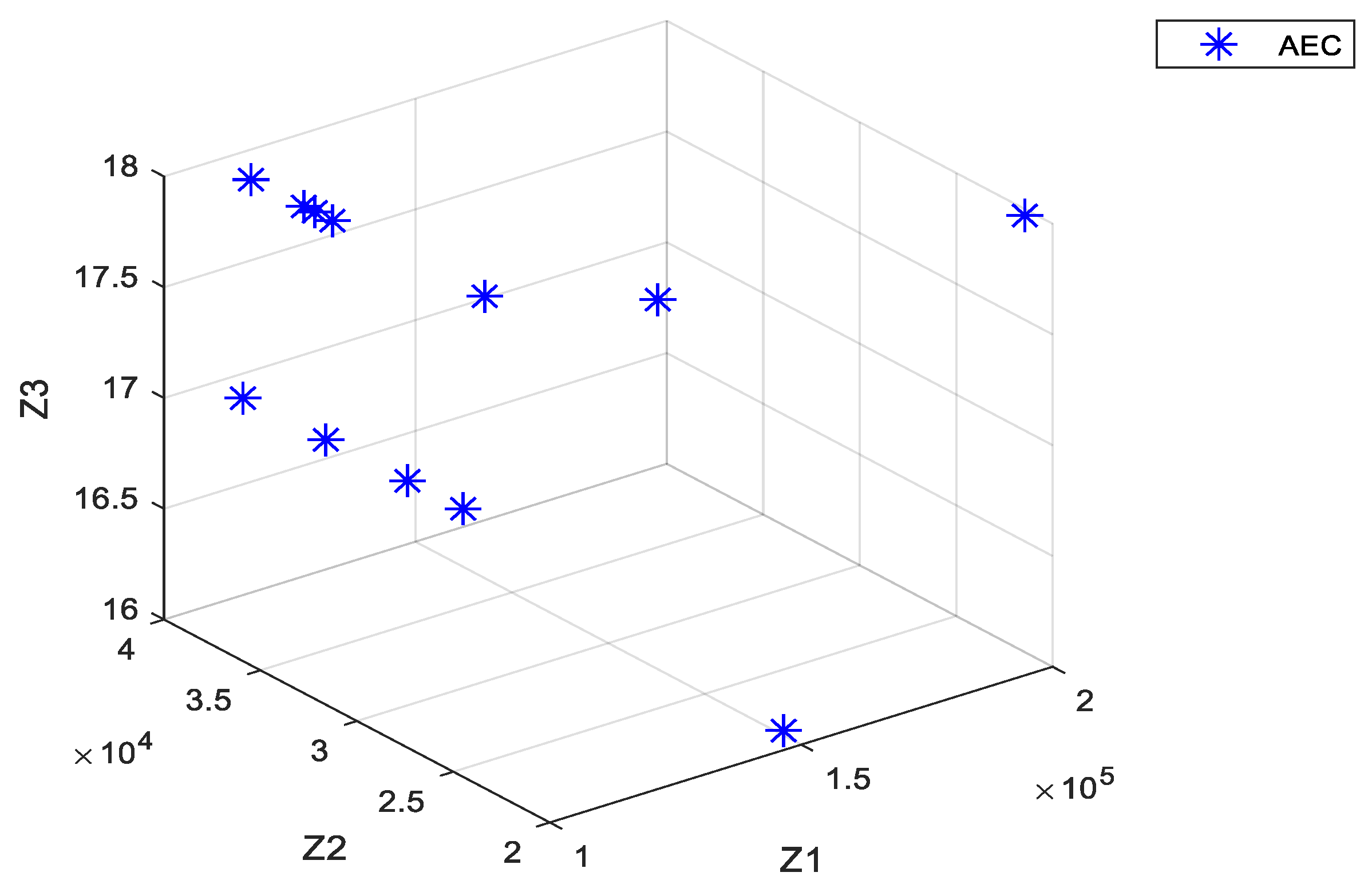
3.3. Solving the Proposed Three-Objective Model with the AEC Approach
3.3.1. Determining the Range of Epsilons’ Values
3.3.2. The AEC Model
4. Numerical Example
4.1. Solving the Problem under Uncertainty Conditions
4.2. Analyzing the Results and Solving the Model Considering the Different Sizes of the Problem
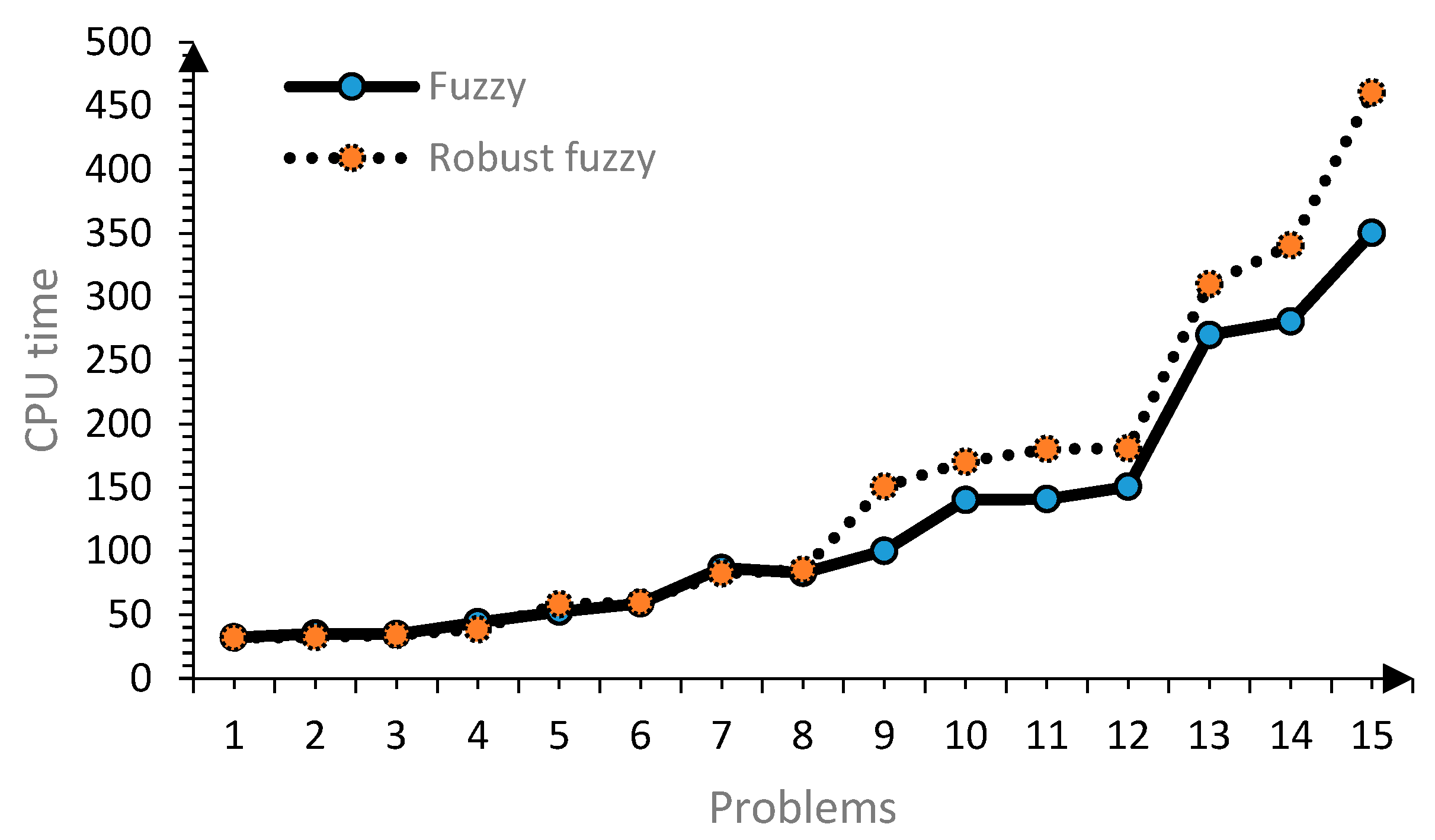
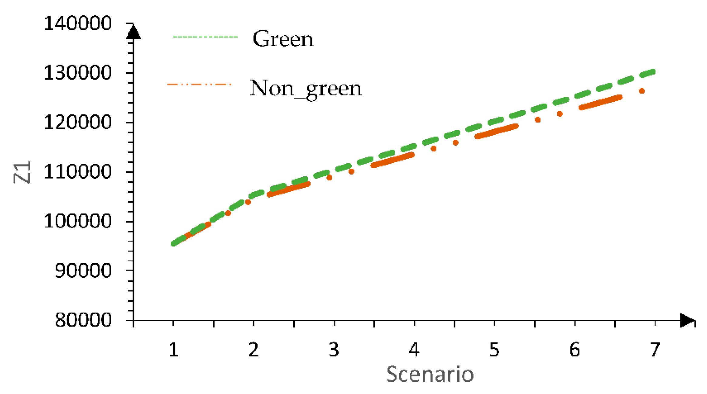
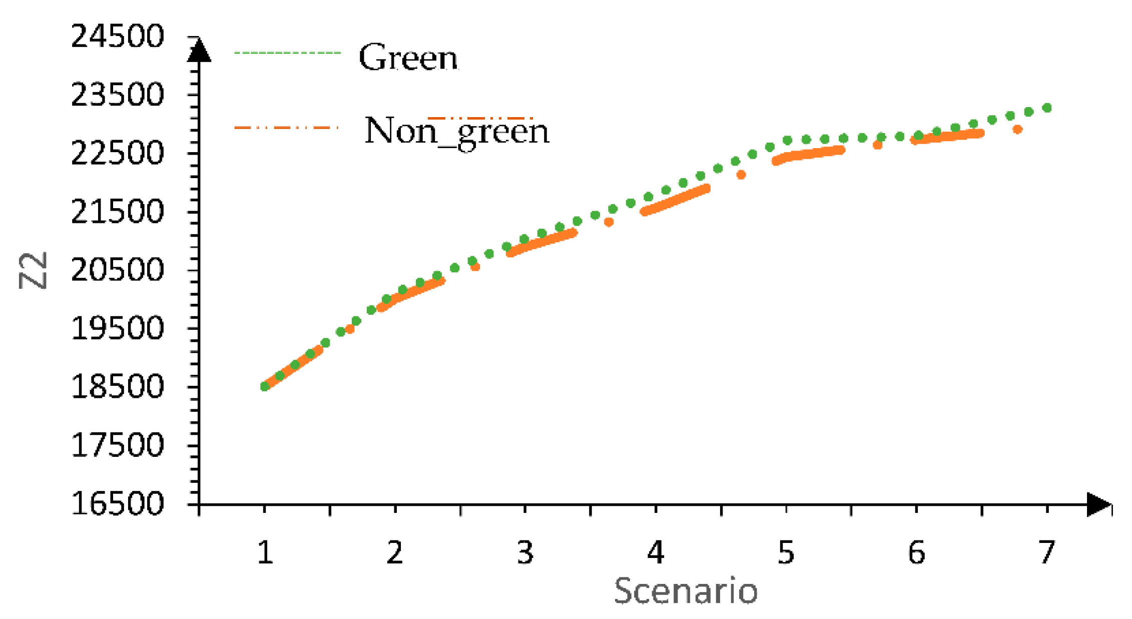
4.3. Analyzing the Results and Solving the Model Considering Various Problems with Different Sizes
5. Discussion
Managerial Discussions and Practical Implications
6. Conclusions
Author Contributions
Funding
Institutional Review Board Statement
Informed Consent Statement
Data Availability Statement
Conflicts of Interest
References
- Guo, C.; Liu, X.; Jin, M.; Lv, Z. The research on optimization of auto supply chain network robust model under macroeconomic fluctuations. Chaos Solitons Fractals 2016, 89, 105–114. [Google Scholar] [CrossRef]
- Sahoo, B.; Poria, S. The chaos and control of a food chain model supplying additional food to top-predator. Chaos Solitons Fractals 2014, 58, 52–64. [Google Scholar] [CrossRef]
- Amin, S.H.; Zhang, G.; Akhtar, P. Effects of uncertainty on a tire closed-loop supply chain network. Expert Syst. Appl. 2017, 73, 82–91. [Google Scholar] [CrossRef] [Green Version]
- Sahebjamnia, N.; Fathollahi-Fard, A.M.; Hajiaghaei-Keshteli, M. Sustainable tire closed-loop supply chain network design: Hybrid metaheuristic algorithms for large-scale networks. J. Clean. Prod. 2018, 196, 273–296. [Google Scholar] [CrossRef]
- Melo, M.T.; Nickel, S.; Saldanha-da-Gama, F. Facility location and supply chain management—A review. Eur. J. Oper. Res. 2009, 196, 401–412. [Google Scholar] [CrossRef]
- Pishvaee, M.S.; Rabbani, M.; Torabi, S.A. A robust optimization approach to closed-loop supply chain network design under uncertainty. Appl. Math. Model. 2011, 35, 637–649. [Google Scholar] [CrossRef]
- Govindan, K.; Soleimani, H. A review of reverse logistics and closed-loop supply chains: A Journal of Cleaner Production focus. J. Clean. Prod. 2017, 142, 371–384. [Google Scholar] [CrossRef]
- Madani, S.R.; Rasti-Barzoki, M. Sustainable supply chain management with pricing, greening and governmental tariffs determining strategies: A game-theoretic approach. Comput. Ind. Eng. 2017, 105, 287–298. [Google Scholar] [CrossRef]
- Tavana, M.; Kian, H.; Nasr, A.K.; Govindan, K.; Mina, H. A comprehensive framework for sustainable closed-loop supply chain network design. J. Clean. Prod. 2022, 332, 129777. [Google Scholar] [CrossRef]
- Guide, V.D.R.; Jayaraman, V.; Linton, J.D. Building contingency planning for closed-loop supply chains with product recovery. J. Oper. Manag. 2003, 21, 259–279. [Google Scholar] [CrossRef]
- Guide, V.D.R.; Van Wassenhove, L.N. The evolution of closed-loop supply chain research. Oper. Res. 2009, 57, 10–18. [Google Scholar] [CrossRef]
- Zhen, L.; Huang, L.; Wang, W. Green and sustainable closed-loop supply chain network design under uncertainty. J. Clean. Prod. 2019, 227, 1195–1209. [Google Scholar] [CrossRef]
- Ma, S.; He, Y.; Gu, R.; Li, S. Sustainable supply chain management considering technology investments and government intervention. Transp. Res. Part E Logist. Transp. Rev. 2021, 149, 102290. [Google Scholar] [CrossRef]
- Ilgin, M.A.; Gupta, S.M. Environmentally conscious manufacturing and product recovery (ECMPRO): A review of the state of the art. J. Environ. Manag. 2010, 91, 563–591. [Google Scholar] [CrossRef] [PubMed]
- Pishvaee, M.S.; Razmi, J.; Torabi, S.A. An accelerated Benders decomposition algorithm for sustainable supply chain network design under uncertainty: A case study of medical needle and syringe supply chain. Transp. Res. Part E Logist. Transp. Rev. 2014, 67, 14–38. [Google Scholar] [CrossRef]
- Tehrani, M.; Gupta, S.M. Designing a Sustainable Green Closed-Loop Supply Chain under Uncertainty and Various Capacity Levels. Logistics 2021, 5, 20. [Google Scholar] [CrossRef]
- Hu, Z.; Parwani, V.; Guiping, H. Closed-loop supply chain network design under carbon subsidies. Comput. Integr. Manuf. Syst. CIMS 2021, 21, 3033–3040. [Google Scholar] [CrossRef]
- Abdi, A.; Fathollahi-Fard, A.M.; Hajiaghaei-Keshteli, M. A set of calibrated metaheuristics to address a closed-loop supply chain network design problem under uncertainty. Int. J. Syst. Sci. Oper. Logist. 2021, 8, 23–40. [Google Scholar] [CrossRef]
- Coskun, S.; Ozgur, L.; Polat, O.; Gungor, A. A model proposal for green supply chain network design based on consumer segmentation. J. Clean. Prod. 2016, 110, 149–157. [Google Scholar] [CrossRef]
- Solér, C.; Bergström, K.; Shanahan, H. Green supply chains and the missing link between environmental information and practice. Bus. Strategy Environ. 2010, 19, 14–25. [Google Scholar] [CrossRef]
- Heidari, A.; Imani, D.M.; Khalilzadeh, M. A hub location model in the sustainable supply chain considering customer segmentation. J. Eng. Des. Technol. 2021, 19, 1387–1420. [Google Scholar] [CrossRef]
- Vali-Siar, M.M.; Roghanian, E. Sustainable, resilient and responsive mixed supply chain network design under hybrid uncertainty with considering COVID-19 pandemic disruption. Sustain. Prod. Consum. 2022, 30, 278–300. [Google Scholar] [CrossRef]
- Meade, L.M.; Sarkis, J.; Presley, A. The theory and practice to Reverse Logistics. Int. J. Logist. Syst. Manag. 2007, 3, 56–84. [Google Scholar] [CrossRef]
- Shekarian, E. A review of factors affecting closed-loop supply chain models. J. Clean. Prod. 2020, 253, 119823. [Google Scholar] [CrossRef]
- Rafigh, P.; Akbari, A.A.; Bidhandi, H.M.; Kashan, A.H. Sustainable closed-loop supply chain network under uncertainty: A response to the COVID-19 pandemic. Environ. Sci. Pollut. Res. 2021. [Google Scholar] [CrossRef]
- Hugo, A.; Pistikopoulos, E.N. Environmentally conscious long-range planning and design of supply chain networks. J. Clean. Prod. 2005, 13, 1428–1448. [Google Scholar] [CrossRef]
- Govindan, K.; Paam, P.; Abtahi, A.R. A fuzzy multi-objective optimization model for sustainable reverse logistics network design. Ecol. Indic. 2016, 67, 753–768. [Google Scholar] [CrossRef]
- Harraz, N.A.; Galal, N.M. Design of Sustainable End-of-life Vehicle recovery network in Egypt. Ain Shams Eng. J. 2011, 2, 211–219. [Google Scholar] [CrossRef] [Green Version]
- Eskandarpour, M.; Dejax, P.; Miemczyk, J.; Péton, O. Sustainable supply chain network design. Omega 2015, 54, 11–32. [Google Scholar] [CrossRef]
- Babazadeh, R.; Razmi, J.; Pishvaee, M.S.; Rabbani, M. A sustainable second-generation biodiesel supply chain network design problem under risk. Omega 2017, 66, 258–277. [Google Scholar] [CrossRef] [Green Version]
- Moradi Nasab, N.; Amin-Naseri, M.R. Designing an integrated model for a multi-period, multi-echelon and multi-product petroleum supply chain. Energy 2016, 114, 708–733. [Google Scholar] [CrossRef]
- Dondo, R.G.; Méndez, C.A. Operational planning of forward and reverse logistic activities on multi-echelon supply-chain networks. Comput. Chem. Eng. 2016, 88, 170–184. [Google Scholar] [CrossRef]
- Varsei, M.; Polyakovskiy, S. Sustainable supply chain network design: A case of the wine industry in Australia. Omega 2017, 66, 236–247. [Google Scholar] [CrossRef]
- Yu, H.; Solvang, W.D. Incorporating flexible capacity in the planning of a multi-product multi-echelon sustainable reverse logistics network under uncertainty. J. Clean. Prod. 2018, 198, 285–303. [Google Scholar] [CrossRef]
- Soleimani, H.; Govindan, K.; Saghafi, H.; Jafari, H. Fuzzy multi-objective sustainable and green closed-loop supply chain network design. Comput. Ind. Eng. 2017, 109, 191–203. [Google Scholar] [CrossRef]
- Roni, M.S.; Eksioglu, S.D.; Cafferty, K.G.; Jacobson, J.J. A multi-objective, hub-and-spoke model to design and manage biofuel supply chains. Ann. Oper. Res. 2016, 249, 351–380. [Google Scholar] [CrossRef]
- Musavi, M.M.; Bozorgi-Amiri, A. A multi-objective sustainable hub location-scheduling problem for perishable food supply chain. Comput. Ind. Eng. 2017, 113, 766–778. [Google Scholar] [CrossRef]
- Peng, H.; Shen, N.; Liao, H.; Xue, H.; Wang, Q. Uncertainty factors, methods, and solutions of closed-loop supply chain—A review for current situation and future prospects. J. Clean. Prod. 2020, 254, 120032. [Google Scholar] [CrossRef]
- Vahdani, B.; Tavakkoli-Moghaddam, R.; Modarres, M.; Baboli, A. Reliable design of a forward/reverse logistics network under uncertainty: A robust-M/M/c queuing model. Transp. Res. Part E Logist. Transp. Rev. 2012, 48, 1152–1168. [Google Scholar] [CrossRef]
- Dehghan, E.; Nikabadi, M.S.; Amiri, M.; Jabbarzadeh, A. Hybrid robust, stochastic and possibilistic programming for closed-loop supply chain network design. Comput. Ind. Eng. 2018, 123, 220–231. [Google Scholar] [CrossRef]
- Fathollahi-Fard, A.M.; Ahmadi, A.; Al-e-Hashem, S.M.J.M. Sustainable closed-loop supply chain network for an integrated water supply and wastewater collection system under uncertainty. J. Environ. Manag. 2020, 275, 111277. [Google Scholar] [CrossRef]
- Khorshidvand, B.; Soleimani, H.; Sibdari, S.; Mehdi Seyyed Esfahani, M. A hybrid modeling approach for green and sustainable closed-loop supply chain considering price, advertisement and uncertain demands. Comput. Ind. Eng. 2021, 157, 107326. [Google Scholar] [CrossRef]
- Sazvar, Z.; Zokaee, M.; Tavakkoli-Moghaddam, R.; Salari, S.A.-S.; Nayeri, S. Designing a sustainable closed-loop pharmaceutical supply chain in a competitive market considering demand uncertainty, manufacturer’s brand and waste management. Ann. Oper. Res. 2021, 1–32. [Google Scholar] [CrossRef] [PubMed]
- Gholizadeh, H.; Fazlollahtabar, H.; Khalilzadeh, M. A robust fuzzy stochastic programming for sustainable procurement and logistics under hybrid uncertainty using big data. J. Clean. Prod. 2020, 258, 120640. [Google Scholar] [CrossRef]
- Fallahpour, A.; Wong, K.Y.; Rajoo, S.; Fathollahi-Fard, A.M.; Antucheviciene, J.; Nayeri, S. An integrated approach for a sustainable supplier selection based on Industry 4.0 concept. Environ. Sci. Pollut. Res. 2021, 1–19. [Google Scholar] [CrossRef] [PubMed]
- Keshavarz Ghorabaee, M.; Amiri, M.; Zavadskas, E.K.; Antucheviciene, J. Supplier evaluation and selection in fuzzy environments: A review of MADM approaches. Econ. Res.-Ekon. Istraz. 2017, 30, 1073–1118. [Google Scholar] [CrossRef]
- Lu, K.; Liao, H.; Zavadskas, E.K. An overview of fuzzy techniques in supply chain management: Bibliometrics, methodologies, applications and future directions. Technol. Econ. Dev. Econ. 2021, 27, 402–458. [Google Scholar] [CrossRef]
- Liu, B.; Iwamura, K. Chance constrained programming with fuzzy parameters. Fuzzy Sets Syst. 1998, 94, 227–237. [Google Scholar] [CrossRef]
- Mavrotas, G. Effective implementation of the e-constraint method in Multi-Objective Mathematical Programming problems. Appl. Math. Comput. 2009, 213, 455–465. [Google Scholar] [CrossRef]
- Aghaei, J.; Amjady, N.; Shayanfar, H.A. Multi-objective electricity market clearing considering dynamic security by lexicographic optimization and augmented epsilon constraint method. Appl. Soft Comput. 2011, 11, 3846–3858. [Google Scholar] [CrossRef]


| Research | Network Structure | Sustainability Aspects | Multi-Product | Types of Customers | Solution Methods | ||||||
|---|---|---|---|---|---|---|---|---|---|---|---|
| Forward | Reverse | Closed-Loop | Economic | Environmental | Social | Main | Variety of Quality | Recycled | |||
| [22] | * | * | * | * | * | * | Heuristic/LR | ||||
| [24] | * | * | CPLEX | ||||||||
| [25] | * | * | * | * | * | * | * | HCC&CF | |||
| [27] | * | * | * | * | * | MOPSO/EC | |||||
| [28] | * | * | * | Lexicograph | |||||||
| [30] | * | * | * | * | AEC | ||||||
| [31] | * | * | * | Heuristic | |||||||
| [19] | * | * | * | * | * | CPLEX | |||||
| [41] | * | * | * | * | * | * | Hybrid method | ||||
| [42] | * | * | * | LR | |||||||
| [43] | * | * | * | Heuristic | |||||||
| Our research | * | * | * | * | * | * | * | * | * | * | Lexicograph/AEC |
, , |
| W = 2 | |||||||
|---|---|---|---|---|---|---|---|
| Customer | Product | Quality Level | TW = 1 | TW = 2 | Quality Level | TW = 1 | TW = 2 |
| 1 | P = 1 | Q = 1 | 117 | Q = 2 | 185 | ||
| 2 | 129 | 122 | |||||
| 3 | 106 | 150 | |||||
| 4 | 200 | 176 | |||||
| 5 | 116 | 125 | |||||
| 6 | 136 | 135 | |||||
| 7 | 159 | 183 | |||||
| 8 | 178 | 130 | |||||
| 1 | P = 2 | 155 | 130 | ||||
| 2 | 135 | 186 | |||||
| 3 | 200 | 158 | |||||
| 4 | 113 | 164 | |||||
| 5 | 167 | 143 | |||||
| 6 | 113 | 115 | |||||
| 7 | 123 | 167 | |||||
| 8 | 111 | 150 | |||||
| Optimal | Obj1 | Obj2 | Obj3 | Epsilon2 | Epsilon3 |
|---|---|---|---|---|---|
| 1 | 110310.1 | 34298.26 | 17 | 34298.26 | 13.508 |
| 2 | 109848.8 | 38474.18 | 17 | 38865.33 | 16.731 |
| 3 | 111084.8 | 27381.6 | 17 | 27381.6 | 11.229 |
| 4 | 110140.2 | 38131.43 | 18 | 38131.43 | 17.838 |
| 5 | 198484.2 | 21043.82 | 18 | 21043.82 | 17.7 |
| 6 | 110581.8 | 34023.52 | 18 | 34023.52 | 17.994 |
| 7 | 110771 | 30186.08 | 17 | 30186.08 | 10.546 |
| 8 | 132514.5 | 22876.38 | 18 | 22876.38 | 16.438 |
| 9 | 110465.1 | 34909.98 | 18 | 34909.98 | 17.854 |
| 10 | 110393.2 | 35457.03 | 18 | 35457.03 | 17.743 |
| 11 | 151137.2 | 21206.96 | 16 | 21206.96 | 12.044 |
| 12 | 111650.8 | 26409.57 | 18 | 26409.57 | 17.808 |
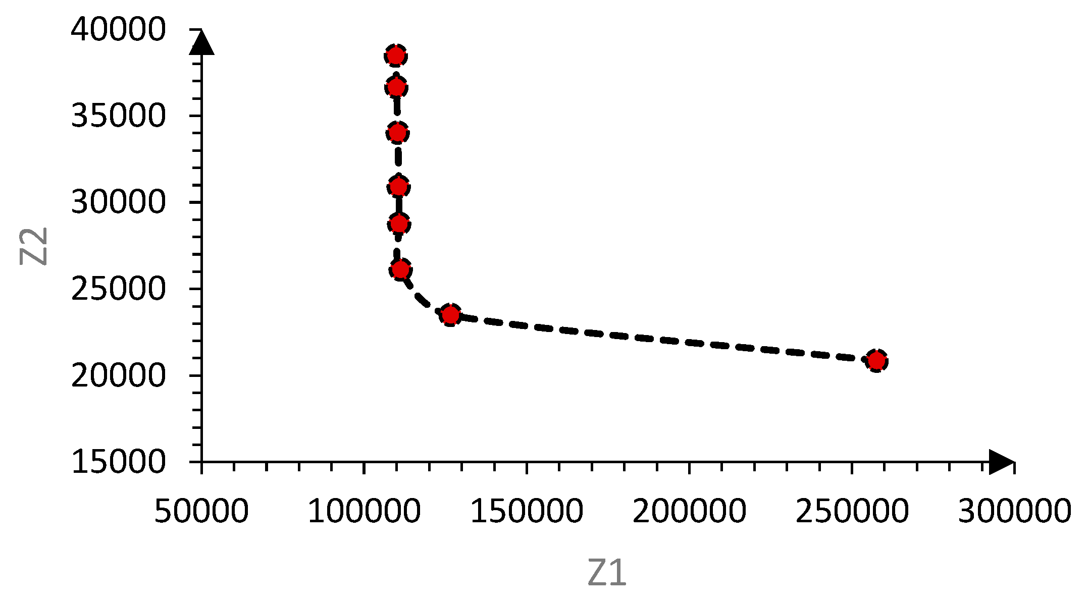
| Optimal | Obj1 | Obj2 | Epsilon2 |
|---|---|---|---|
| 1 | 257609.1 | 20858.02 | 20858.02 |
| 2 | 126651 | 23489.32 | 23489.32 |
| 3 | 111254.8 | 26120.62 | 26120.62 |
| 4 | 110846.1 | 28751.91 | 28751.91 |
| 5 | 110681 | 30897.68 | 31383.21 |
| 6 | 110316.6 | 34014.51 | 34014.51 |
| 7 | 109922.1 | 36645.81 | 36645.81 |
| 8 | 109803.8 | 38474.18 | 39277.11 |
| Optimal | Obj1 | Obj3 | Epsilon3 |
|---|---|---|---|
| 1 | 109956.5 | 18 | 18 |
| 2 | 109956.5 | 18 | 17.556 |
| 4 | 109686.7 | 17 | 16.667 |
| 5 | 109666.3 | 16 | 15.778 |
| 6 | 109662.1 | 15 | 14.889 |
| 7 | 109641.7 | 14 | 14 |
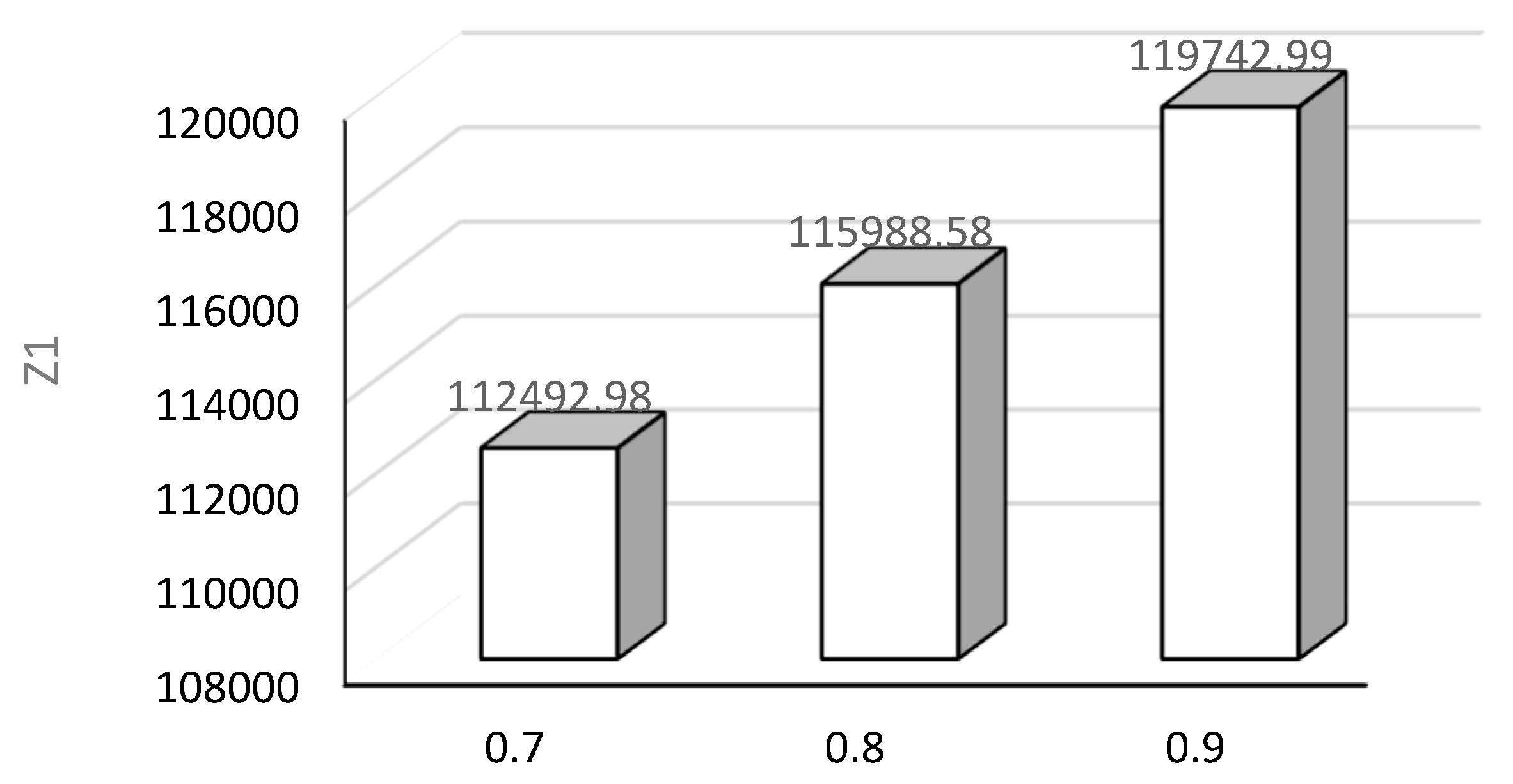
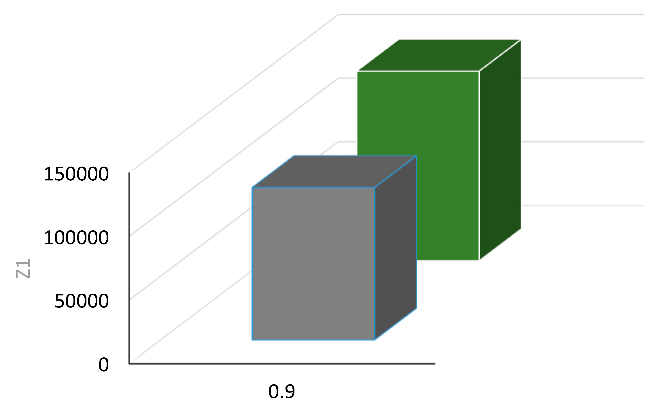
| Possibilistic Programming | Robust Possibilistic Programming | ||||||
|---|---|---|---|---|---|---|---|
| α, β, λ | Obj1 | Obj2 | Obj3 | Obj1 | Obj2 | Obj3 | |
| 1 | 0.7 | 112492.98 | 36736.85 | 17 | 149040.568 | 44036.731 | 17 |
| 2 | 0.8 | 115988.58 | 42318.86 | 17 | |||
| Factory (Potential) | Warehouse (Potential) | Customers | Collection Centers | Disposal Centers | Transportation Mode for Factory | Transportation Mode for Warehouse | Transportation Mode for Customers | Transportation Mode for Collection Centers | Transportation Mode for Disposal Centers | Product | Quality | |
|---|---|---|---|---|---|---|---|---|---|---|---|---|
| Sample Problem | F | W | C | I | N | TF | TW | TK | TI | TN | P | Q |
| 1 | 3 | 2 | 8 | 3 | 3 | 2 | 4 | 3 | 4 | 2 | 2 | 2 |
| 2 | 3 | 5 | 12 | 3 | 3 | 2 | 4 | 3 | 4 | 2 | 2 | |
| 3 | 3 | 5 | 14 | 3 | 3 | 2 | 4 | 3 | 4 | 2 | 2 | |
| 4 | 3 | 9 | 16 | 4 | 4 | 2 | 4 | 3 | 4 | 2 | 3 | |
| 5 | 4 | 9 | 18 | 4 | 4 | 3 | 5 | 4 | 4 | 2 | 3 | |
| 6 | 4 | 9 | 20 | 4 | 4 | 3 | 5 | 4 | 5 | 3 | 3 | |
| 7 | 4 | 11 | 22 | 5 | 5 | 3 | 5 | 4 | 5 | 3 | 4 | |
| 8 | 5 | 11 | 24 | 5 | 5 | 3 | 5 | 4 | 5 | 3 | 4 | |
| 9 | 5 | 11 | 26 | 5 | 5 | 4 | 6 | 5 | 5 | 3 | 4 | |
| 10 | 5 | 13 | 28 | 6 | 6 | 4 | 6 | 5 | 5 | 3 | 5 | |
| 11 | 6 | 13 | 30 | 6 | 6 | 4 | 6 | 5 | 6 | 4 | 5 | |
| 12 | 6 | 13 | 32 | 6 | 6 | 4 | 6 | 5 | 6 | 4 | 5 | |
| 13 | 6 | 15 | 34 | 7 | 7 | 4 | 7 | 6 | 6 | 4 | 6 | |
| 14 | 8 | 15 | 36 | 7 | 7 | 5 | 7 | 6 | 6 | 4 | 6 | |
| 15 | 8 | 15 | 38 | 7 | 7 | 5 | 7 | 6 | 6 | 4 | 6 |
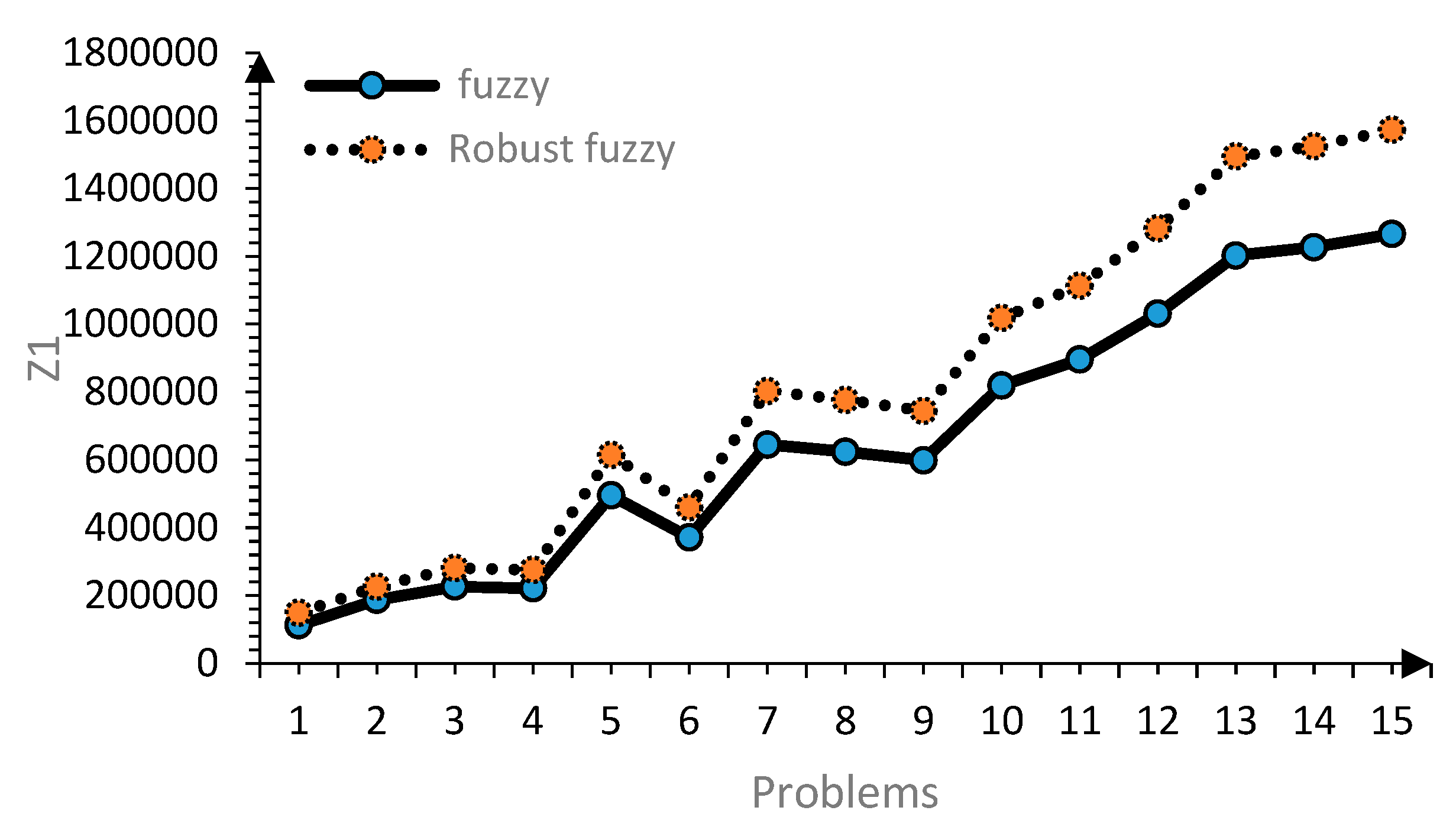
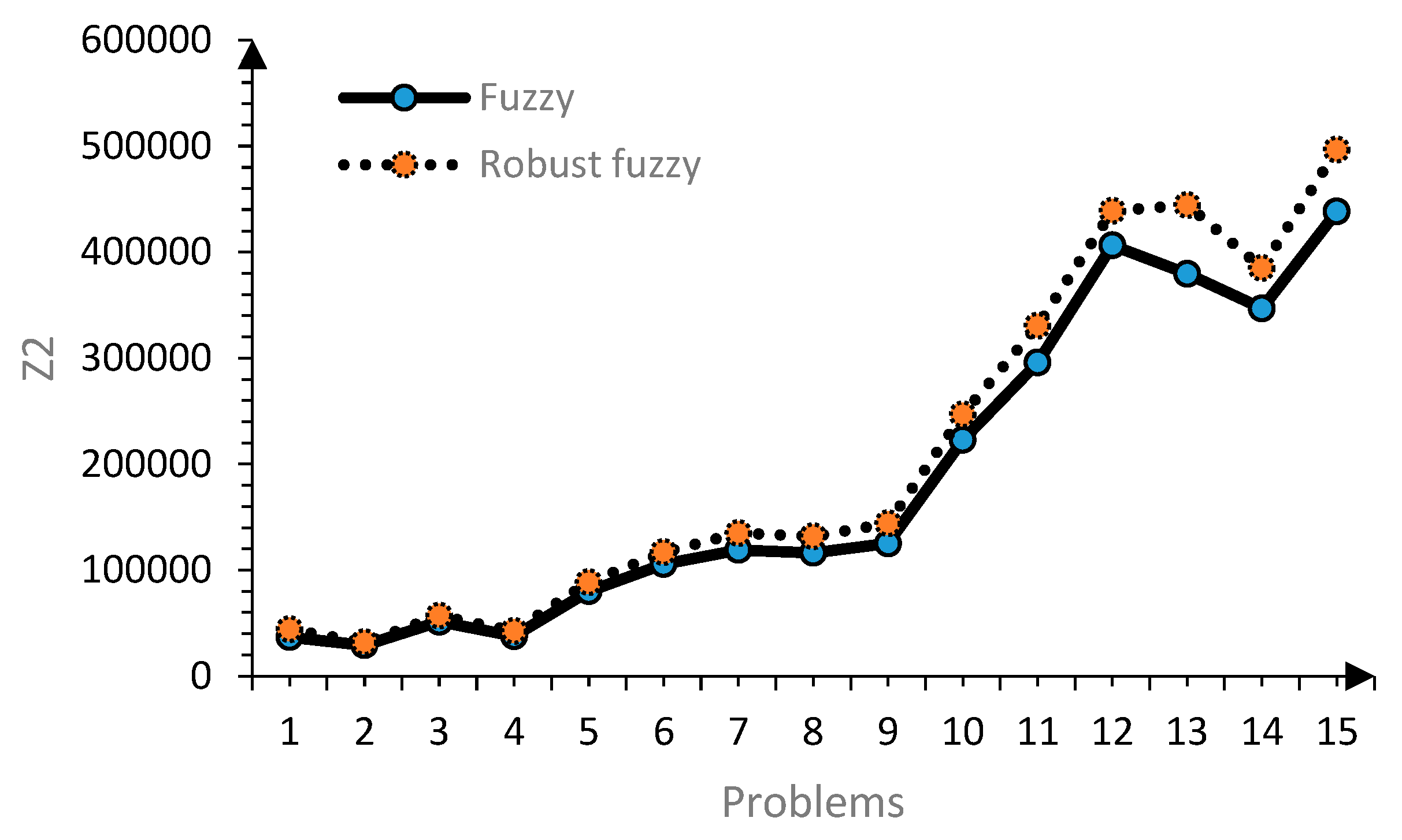
| Possibilistic Programming | Solution Time | Robust Possibilistic Programming | Solution Time | |||||
|---|---|---|---|---|---|---|---|---|
| Obj1 | Obj2 | Obj3 | Obj1 | Obj2 | Obj3 | |||
| 1 | 112493 | 36736.85 | 17 | 32.2 | 149040.6 | 44036.73 | 17 | 31.8 |
| 2 | 187169 | 29267.91 | 29 | 35.1 | 226106 | 31864.99 | 29 | 32.3 |
| 3 | 226508.6 | 51318.52 | 30 | 34.6 | 280990.5 | 56885.9 | 30 | 34 |
| 4 | 221298.8 | 37652.39 | 35 | 43.95 | 275637.5 | 42646.97 | 35 | 38.5 |
| 5 | 495118.2 | 79996.83 | 44 | 52.3 | 614204.3 | 88622.48 | 41 | 58.3 |
| 6 | 371434.2 | 105694.7 | 44 | 58.9 | 459974.3 | 116882 | 44 | 59.7 |
| 7 | 645098.4 | 119017.6 | 45 | 86.7 | 802963.3 | 134888 | 44 | 82.4 |
| 8 | 623957.8 | 116261.9 | 57 | 82.8 | 776619 | 131765.5 | 57 | 85.3 |
| 9 | 598870.6 | 125125.3 | 56 | 10.2 | 744473.2 | 144066.5 | 55 | 15.65 |
| 10 | 819076.4 | 222814.6 | 61 | 14.28 | 1017886 | 246844 | 61 | 17.32 |
| 11 | 895641.9 | 295736.8 | 83 | 14.78 | 1113248 | 330478.7 | 83 | 18.2 |
| 12 | 1031021 | 406372.7 | 57 | 15.6 | 1282136 | 438746.5 | 57 | 18.8 |
| 13 | 1202309 | 379571.3 | 83 | 27 | 1494380 | 444382.5 | 82 | 31 |
| 14 | 1226793 | 346850.2 | 75 | 28.7 | 1524536 | 385002.7 | 75 | 34.6 |
| 15 | 1265524 | 438293.4 | 73 | 35.2 | 1572802 | 496758.6 | 73 | 46.7 |
| Non-Green Customers | Green Customers | |||||||||
|---|---|---|---|---|---|---|---|---|---|---|
| Scenario | Obj1 | Obj2 | Obj3 | Epsilon2 | Epsilon3 | Obj1 | Obj2 | Obj3 | Epsilon2 | Epsilon3 |
| 0 | 95502.610 | 18508.589 | 17 | 18508.589 | 17 | 95502.610 | 18508.589 | 17 | 18508.589 | 17 |
| 0/2 | 104548.366 | 20015.360 | 17 | 20015.360 | 18 | 105380.050 | 20116.889 | 17 | 20116.889 | 18 |
| 0/3 | 109068.938 | 20903.887 | 17 | 20903.887 | 17 | 110324.145 | 21042.220 | 17 | 21042.220 | 17 |
| 0/4 | 113590.680 | 21565.449 | 17 | 21776.655 | 18 | 115270.113 | 21801.261 | 17 | 21976.472 | 18 |
| 0/5 | 118091.996 | 22440.993 | 17 | 22664.224 | 17 | 120206.676 | 22727.276 | 17 | 22908.389 | 17 |
| 0/6 | 122613.476 | 22735.056 | 17 | 22135.056 | 18 | 125164.781 | 22800.815 | 17 | 22400.815 | 18 |
| 0/7 | 127115.501 | 22970.552 | 17 | 22970.552 | 17 | 130409.262 | 23284.226 | 17 | 23284.226 | 17 |
Publisher’s Note: MDPI stays neutral with regard to jurisdictional claims in published maps and institutional affiliations. |
© 2022 by the authors. Licensee MDPI, Basel, Switzerland. This article is an open access article distributed under the terms and conditions of the Creative Commons Attribution (CC BY) license (https://creativecommons.org/licenses/by/4.0/).
Share and Cite
Soon, A.; Heidari, A.; Khalilzadeh, M.; Antucheviciene, J.; Zavadskas, E.K.; Zahedi, F. Multi-Objective Sustainable Closed-Loop Supply Chain Network Design Considering Multiple Products with Different Quality Levels. Systems 2022, 10, 94. https://doi.org/10.3390/systems10040094
Soon A, Heidari A, Khalilzadeh M, Antucheviciene J, Zavadskas EK, Zahedi F. Multi-Objective Sustainable Closed-Loop Supply Chain Network Design Considering Multiple Products with Different Quality Levels. Systems. 2022; 10(4):94. https://doi.org/10.3390/systems10040094
Chicago/Turabian StyleSoon, Amirhossein, Ali Heidari, Mohammad Khalilzadeh, Jurgita Antucheviciene, Edmundas Kazimieras Zavadskas, and Farbod Zahedi. 2022. "Multi-Objective Sustainable Closed-Loop Supply Chain Network Design Considering Multiple Products with Different Quality Levels" Systems 10, no. 4: 94. https://doi.org/10.3390/systems10040094
APA StyleSoon, A., Heidari, A., Khalilzadeh, M., Antucheviciene, J., Zavadskas, E. K., & Zahedi, F. (2022). Multi-Objective Sustainable Closed-Loop Supply Chain Network Design Considering Multiple Products with Different Quality Levels. Systems, 10(4), 94. https://doi.org/10.3390/systems10040094