
Method of Software Development Project Duration Estimation for Scrum Teams with Differentiated Specializations


Department of Automated Control Systems, Computer Science and Information Technologies Institute, Lviv Polytechnic National University, 79000 Lviv, Ukraine
*
Author to whom correspondence should be addressed.
Systems 2022, 10(4), 123; https://doi.org/10.3390/systems10040123
Submission received: 22 July 2022
/
Revised: 10 August 2022
/
Accepted: 14 August 2022
/
Published: 17 August 2022
(This article belongs to the Special Issue Decision-Making Process and Its Application to Business Analytic)
Abstract
:Estimation is an essential step of software development project planning that has a significant impact on project success—underestimation often leads to problems with the delivery or even causes project failure. An important aspect that the classical estimation methods are usually missing is the Agile nature of development processes in the implementation phase. The estimation method proposed in this article aims at software development projects implemented by Scrum teams with differentiated specializations. The method is based on the authors’ system of working-time balance equations and the approach to measuring project scope with time-based units—normalized development estimates. In order to reduce efforts spent on the estimation itself, an analysis of dependencies among project tasks is not mandatory. The outputs of the methods are not recommended to be treated as commitments; instead, they are supposed to be used to inform project stakeholders about the forecasted duration of a potential project. The method is simple enough to allow even an inexpensive spreadsheet-based implementation.
1. Introduction
Software development technologies are evolving fast, addressing various challenges modern businesses are faced with. Being an integral part of the software development toolset, estimation techniques also have to fulfill the constantly changing requirements appropriately. Quite often, one of the main reasons for a project’s unsuccess or event failure is inappropriate estimation. Primarily, it is an underestimation of required development efforts and, consequently, far too optimistic deadlines and budgets. Starting from the middle of the 20th century, there have been a large number of estimation methods, the most famous of which are PERT [1], CPM [2], FPA [3], COCOMO [4,5,6,7], and Scrum Poker [8]. However, the already existing well-known methods do not fully take into account the fact that the future implementation of estimating projects is going to be done following Agile-like methodologies. Therefore, the creation of estimation methods that take into account the Agile nature of software development processes is a relevant scientific task.
The goal of the study is to develop a method of intermediate estimation of software development project duration supposed to be implemented by Scrum teams with differentiated specializations. Under the intermediate estimation, it is understood to be an estimation stage occupying the place between the preliminary evaluation (similar to a rough order of magnitude [9] which is performed in the earliest project phases) and precise estimation (or definite estimate [9] that takes place before project implementation start). The “differentiated specializations” means that each software developer performs tasks of a certain specialization and does not do tasks from the other specializations.
To achieve the goal of the study the following tasks have been done: defined an approach to measure project scope as well as the development capacity of a Scrum team; created a system of equations that reflects the structuring of software developers working time taking into account competency levels and specializations of team members as well as their involvement in the project; defined steps of the method; demonstrated usage of the method by an example.
The proposed method ensures estimating the duration of a software project providing as the output a project release plan that represents optimistic and pessimistic scenarios of project implementation. Importantly, the method ensures minimizing the working time spent on the estimation itself. It is also worth noting that the outcomes received by applying the method are not recommended to be used to make commitments (e.g., when signing a contract with the client); instead, the outcomes can be used in further project stages—precise estimation and implementation monitoring. Software implementation of the method does not require a sophisticated toolset—in the simplest scenario, the implementation can be done as a spreadsheet (e.g., MS Excel, Google Sheets, etc.); according to the authors’ vision, the method is going to be included in the software product [10].
2. Literature Review
Estimation methods have been evolving along with the entire software development industry starting from the second half of the 20th century. In this section, we provide a brief overview of the most famous estimation techniques including the ones related to the method proposed in this study.
One of the oldest and most used estimation methods is the Program Evaluation and Review Technique (PERT) which was developed by the United States Navy [1] and then adopted in other industries including software development. The method combines expert evaluation of estimable items providing the so-called three-point estimates for optimistic, pessimistic, and the most likely scenarios as well as statistics-based techniques that allow calculating the final estimate. Additionally, the method includes approaches to monitor the implementation process and adjust the plan accordingly to the remaining efforts and time. One of the most significant weaknesses of PERT is that it does not take into account the Agile nature of modern software development processes. It is recommended to use the three-point estimation technique of the PERT in the first step of the method proposed in the current article.
Another well-known method often applied in conjunction with PERT is the Critical Path Method (CPM) [2] which is intended for estimating the duration of a project as the duration of the longest project task path. Usage of the method requires a task breakdown structure and analysis of dependencies among the tasks. The CPM is quite useful for definite estimation [9] when its outcomes are supposed to be used as commitments. Since applying the method requires a highly detailed project scope, it is not suggested to use the method in the early stages of project estimation and planning.
The Graphical Evaluation and Review Technique (GERT) [11] is based on a more advanced network analysis than PERT or CMP. This method allows combining the probabilistic nature of network logic (i.e., dependencies between project tasks) and effort estimates. GERT is usually applicable to the planning of complex projects.
Published in the late 1970s, the Putnam model [12,13] was one of the first model-based estimation techniques. It uses the Rayleigh distribution to establish interrelation among such variables as software size (expressed in so-called effective lines of code), efforts (working time spent on the development measured in man-hours), and duration (project schedule). This estimation technique is also well-known as SLIM (Software Lifecycle Management) [14] which, in turn, is the name of the proprietary suite that implements the Putnam model.
The Functional Point Analysis (FPA) method [3] is founded on the idea of measuring the size of software in so-called function points that express the “amount” of delivered external functionality (not taking into account internal technology aspects). The Use Case Points (UCP) method [15] is based on similar principles as FPA except that a use case is chosen as the object of measurement (the “use case” term is used in the same meaning as in Unified Modeling Language). To this family of estimation methods also belongs the Software Non-functional Assessment Process (SNAP) [16] that, in contradiction to FPA, measures non-functional requirements. In practice, FPA and SNAP can complement each other since the first one targets functional requirements whilst the second one focuses on non-functional aspects. All three methods use historical data collected either in the industry or within a particular organization to convert the value of software size expressed in “points” to time-based units (e.g., man-hours).
The Constructive Cost Model (COCOMO) [4,5] method was introduced in the early 1980s. This method allows calculating development efforts, average team size, and project duration based on the LOC (number of lines of code) metric. COCOMO proposes three models depending on the level of details and required estimates accuracy: basic, intermediate, and detailed. Additionally, the method takes into account the level of project complexity as well as creativity and experience expected from a development team. The most questionable part of the method is still the usage of the LOC metric since the number of lines of source code significantly depends on a programming language, coding guidelines, used frameworks, and development tools.
Introduced in the late 1990s, the COCOMO II [6,7] method became the next evolutionary step of COCOMO. It includes three sub-models depending on the type of software developed: end-user programming, intermediate sector (application generators, application compositions, system integration), and infrastructure. The method differentiates estimates according to the project phase: stage I (prototyping), stage II (early design phase), and stage III (post architecture design phase). Unlike its predecessor, the COCOMO II method mitigates the level of risk and, in addition to the LOC metric, uses also function and object points.
Along with the widespread of Agile methodologies, various Agile-oriented estimation techniques have become popular. One of the most commonly used is Planning Poker (also known as Scrum Poker) [8]. However, it should be emphasized that the following methods (similar to Planning Poker) [17] are also widespread: T-Shirt size estimation, Dot Voting, Bucket System, Large/Uncertain, Small, etc. An interesting aspect of these methods is the usage of story points (or their analogs) to estimate development efforts and measure the productivity (or velocity) of an Agile team [18]. Another important peculiarity of these techniques is that they are heavily based on the expert judgment of a team. On the one hand, this ensures the involvement of a team in project planning. On the other hand, usage of these methods is not possible before starting project implementation (e.g., in the analysis and design phase) when a team is not built yet. Such drawbacks of the Planning Poker-like methods are addressed in the Constructive Agile Estimation Algorithm (CAEA) [19,20] which combines story point-based sizing with the algorithmic part dividing the estimation process into two phases—early estimation and iterative estimation (an example of using CAEA is represented in the estimation framework from [21]). As shown in [22,23], the current research efforts aiming at estimation in Agile software development are mainly directed to such categories of techniques as machine learning-based, expert judgment, and algorithmic. Further information about estimation in Agile software development can be found in [24,25].
A separate area of research is improving the existing estimation methods with machine learning techniques. The following studies can be mentioned as relevant examples of this trend: fuzzy theory dealing with uncertainty [26,27]; the Bayesian network improving PERT [28]; optimization of COCOMO parameters with the Genetic algorithm [29]; improving prediction values of UCP with the random forest technique [30]. Overviews of usage of machine learning in the software project estimation area can also be found in [31,32].
According to the survey [33], the vast majority of the respondents use expert judgment for estimation; parametric models, such as variations of FPA and COCOMO, take the second position among the participants. As the survey shows, time-based units (e.g., man-hour) are the most used units of measurement; story points occupy the second position in the rating. A summary of the estimation techniques overview (including the method proposed by the authors, row #12) is provided in Table 1.
The method of estimating project duration proposed in the current study is supposed to be used in conjunction with expert judgment (e.g., the three-point estimation of PERT) in order to receive so-called normalized development estimates (NDE) expressed in time-based units, preferably, man-hours (see definition of the NDE term below). Calculation of the project duration is based on the structuring of software developers working time and sprint-based release planning (which makes the difference with CPM that requires a detailed analysis of dependencies among project tasks). The current version of the method does not require any explicit usage of historical data, instated, it uses the experience of the experts involved in the estimation. In the future, when enough historical data are accumulated, improved versions of the method can be created.
3. Results
3.1. Structuring of Software Developer Working Time
Let W be the working time that a software developer spends being assigned to a project. Project working time, W, can be divided into parts such as project scope implementation, M, which is part of working time spent for developing project features (it also includes team collaboration related to the development); working time spent on general project activities, G, including project meetings (daily stand-ups, sprint plannings, demos, retrospectives, etc.), environment setup at the beginning, project stabilization before releasing; non-working time, N, when a developer does not do any real project work (vacations, sick leaves, day offs, waiting time while being blocked by dependencies). Hence, project working time, W, can be expressed as the sum of the three components mentioned above:
Typically, to implement a software project, it is necessary to combine a few programming technologies (e.g., back-end, front-end, database). A particular software developer can be a specialist in a single programming technology or be able to do tasks belonging to different technologies (usually, back-end engineers also do database tasks, or so-called full stack developers perform both front-end and back-end tasks). Let project scope implementation working time belonging to technology s, , consist of two major components: development working time (DWT), , and supplementary development activities . Component is the working time that a software developer spends on coding only excluding supplementary development activities, , such as team collaboration, defect fixing, writing unit tests, etc. Therefore, project scope implementation working time, M, is expressed by the following equation:
where q is the number of development specializations in the team.
Under a Scrum team with differentiated specializations, it is understood a Scrum team each developer of which can perform tasks of only 1 specialization: if a software developer j has specialization , then and for . In turn, if there are members of a Scrum team who can perform tasks of more than one specialization, the team is called a Scrum team with mixed specializations (such teams are out of the scope of the current study).
The non-working time component, N, can be split into two completely different subcomponents: leave time, O, which includes planned vacations, days off, sick leaves, etc.; idle time, I, when a software developer cannot do project tasks due to, for example, lack of project tasks or being blocked by unresolved dependencies. It is worth noting that non-working time does not include days excluded from the working calendar (e.g., weekends or state holidays). Then, the equation expressing non-working time, N, is the following:
Combining (2) and (3), Equation (1) is written as:
By the definition, variables from (4) are greater than or equal to 0: , , , , , and . The basic measurement unit for these variables is the man-hour.
Given that a development team consists of n members, and a project lasts for k sprints, it implies from (4) that the equation applicable for a particular software engineer from the team is:
where i is a sequence number of a sprint, j is an identifier of a software developer. Additionally, to have a possibility to intentionally exclude development activities for a certain sprint, team member, or specialization, it is introduced parameter with two possible values: if , project scope development is included into sprint i for developer j and specialization s; if , otherwise. For example, if is a stabilization sprint (that includes final defect fixing found during regression testing and preparing software components for releasing), development of new project scope is not supposed to take place, therefore, .
Let be duration of sprint i (expressed in hours). For example, in the case of a sprint lasting 2 weeks (i.e., 10 days for 8 h each), h (of course, if no state holidays within the 2 weeks). The relationship between project working time, , and sprint duration, , is expressed by the equation:
where is an involvement coefficient of developer j into sprint i:
where is the maximum possible value of the involvement coefficient limited by the higher allowed boundary for overtimes. Since regular overtimes cause decreases in the productivity of individual team members (that even may affect the productivity of the whole team), considering overtimes in estimates is a question rather related to risk management, therefore, it is out of the scope of the current study.
3.2. Normalized Development Estimates
For estimation and further project implementation monitoring, it is important to have a unified measure of project scope size. Let an “average” software developer (ASD) be a software developer who is competent enough (i.e., possesses the required knowledge, skills, and experience) to act as a player of a development team performing a certain type (or types) of tasks with an acceptable level of quality without permanent supervision from more skillful colleagues and, at the same time, still has some space for improvement of the competency level, first of all, in terms of efficiency and complexity of the work done. The closest position to the “average” software developer defined in competency matrices of software development companies is the position of a middle software engineer.
Let U be the normalized development working time (NDWT) which is the DWT spent by an ASD on implementing a certain amount of project scope. If D is DWT spent by another developer on the tasks, then the following expression takes place:
where is a productivity coefficient (PC); in turn, is a competency level productivity coefficient (CLPC), and is an involvement productivity coefficient (IPC). For an ASD, ; if a competency level is lower than ASD, then ; if a competency level is higher than ASD, ; if a developer is not competent in a certain specialization. In turn, coefficient depends on the involvement, :
The normalized development capacity (NDC), C, is the maximum possible value of NDWT that can be spent on project scope implementation:
where is a set of all possible values of NDWT, U. In essence, NDC expresses the maximum possible amount of scope that can be implemented by a particular developer or the whole team within a certain time range (e.g., project sprint). Drawing the parallels with the Agile estimation techniques [8,17,18,19], NDC is nothing else as a forecast of the velocity of a Scrum team expressed in time-based units. For a development team with differentiated specializations, NDC is defined as a vector each item of which corresponds to a particular specialization:
where NDC for a particular specialization is a sum of NDCs of each software developer for all the sprints:
Considering (7), NDC for developer j on sprint i for specialization s is defined as follows:
where and are sets of all possible values of NDWT and DWT respectively for developer j on sprint i for specialization s.
The normalized development estimate (NDE), E, of a certain project scope is a forecast of DWT supposing that the work is done by an ASD. In other words, the NDE, E, is a forecast of NDWT, U. One of the main purposes of both terms is to unify the measurement of the amount of project scope expressing it in time-based units (e.g., man-hours). It is assumed that NDE can result from expert evaluations (e.g., the three-points estimation of PERT).
Since the implementation of a project requires joint efforts of several specializations, NDE has to be provided for each specialization separately:
where is NDE for specialization s; q is the number of specializations; is a vector of NDEs for the whole project. Considering (7), the NDE, , is expressed as follows:
where is CLPC of developer j for specialization s; is an IPC for developer j on sprint i. It is worth emphasizing the assumption that the competency levels of the software developers are not changed during the project, i.e., parameters do not depend on a project sprint, i.
3.3. System of Working Time Balance Equations
After combining (5), (6), and (10), it implies the following system of working time balance equations:
Assuming that working time spent on supplementary development activities, , proportionally depends on development working time, , we receive the expression:
where a supplementary development activities coefficient (SDAC), , can change along with the project implementation (e.g., on project start, a portion of supplementary development activities is higher due to, for example, the necessity to get familiar with project tasks and build as a team); also, depends on peculiarities of a specialization (e.g., back-end development requires writing unit tests whilst database development usually does not).
Similarly to (12), given that general project activities, , proportionally depends on a project’s working time, , deducting the leave time, (a developer on a leave cannot participate in general project activities):
where is a general project activities coefficient (GPAC) that might vary depending on the project phase (e.g., usually, the coefficient values are higher on project start and finish).
It is worth noting that coefficients and reflect, in particular, the amount of working time spent on team collaboration. Therefore, the coefficients have to take into account a team-building lifecycle (in Scrum, they are usually applied to the model that defines such stages as forming, storming, norming, performing, and adjourning [35]). A study of the dependence of coefficients and on the team development stage is out of scope.
Substituting in (11) variables and expressed by (12) and (13) respectively, we get a modified version of the system of working time balance equations:
If a software developer j has specialization , then , and for . Hence, the first equation of system (14) can be written as follows:
From (15) and (6), it is possible to get an expression to calculate DWT for developer j (that possesses specialization ):
which, in turn, leads to the expression for NDC:
where and are sets of all possible values of leave time and idle time respectively for developer j on sprint i.
3.4. Project Duration Estimation Criteria
Let be the NDE, and be a minimum number of sprints required to implement a project. Then, the estimated duration of the project, , has to fulfill the following criteria:
where is NDC for specialization s if a project lasts k sprints.
3.5. Method Algorithm
To apply the method, it is necessary to perform the four steps specified in the current section below. In order to improve the quality of the estimate, steps 1–4 can be iteratively repeated a few times tuning the parameters on each iteration.
3.5.1. Step 1. Normalized Development Estimates
The current step is about the sizing of the project scope. A similar step is included in the other methods, as well. The main difference is how the sizing is done (expertise-based, model-based, etc.) and in what units the project scope is measured (LOC, function points, story points, man-hours, etc.). In terms of the sizing approach, the proposed method is the closest to the PERT technique [1].
The goal of this step is to size the project scope as a range receiving two versions of NDEs for the optimistic and pessimistic scenarios:
where and are optimistic and pessimistic NDEs correspondingly for specialization s; q is a number of specializations.
Typically, to prepare the NDE, an expert evaluation approach can be applied, for instance, the PERT-based three-point estimation. Methods of preparing the NDE itself are out of the scope of the current study.
3.5.2. Step 2. Release Planning
The current step is based on the ideas of Scrum sprint planning with the difference that, instead of story point-based velocity, NDC expressed in man-hours is used [21,22,23].
This step targets splitting project implementation into phases and specifying parameters for each of the phases. It consists of the following sub-steps:
- 1.
- Define the duration of a sprint, . As a rule, sprint duration is 2 weeks (or 80 working hours). However, it is necessary to take into account state holidays. Given that, on average, there is 1 state holiday per month, an average duration of a sprint is 76 working hours.
- 2.
- Split project implementation into phases. In this context, a project phase is a sequence of adjacent sprints united by certain intermediate goals, the same values of parameters (e.g., GPAC, , where p is an identifier of a phase), and team composition. Typical project phases are as follows: project start, team scaling, performing, stabilization, user acceptance testing, and releasing. It recommended that project phases reflect the team development stages [35].
- 3.
- Specify project scope development flag, . For example, on project start, apart from general project activities (such as setting up project infrastructure), implementation of project scope is planned. In contrast, in the stabilization and the subsequent phases, project scope development does not take phase.
- 4.
- Define number of sprints for each phase including the total number of sprints as well as the number of mandatory sprints (a mandatory sprint is a sprint that takes place regardless of the availability of the project scope to implement). For instance, the project start phase includes two sprints that are mandatory. In turn, the duration of the performing phase (where the main part of development is done) is unknown in the current step—it is found in Step 4.
- 5.
- Provide GPAC, . Values of the coefficient are usually higher in the beginning phases in comparison with the performing phase where the development team is already built and focused rather on project scope development than on general project activities. In the finalization phases, the values of the coefficient are equal to 1 since the team does only general project activities (e.g., fixing defects after regression testing, which is not the development of the project scope).
- 6.
- Specify SDAC, , for each specialization. It is worth noting that the coefficient includes such activities as writing unit tests, fixing defects related to a particular project scope item, as well as team collaboration related to development (e.g., technical meetings). The coefficient is applicable only for phases where development of project scope (i.e., ) takes place. Like , coefficients have the lowest value on the performing phase where productivity of the development team is the highest.
3.5.3. Step 3. Development Team Composition
This step aims to define the composition of the development team as well as specify the related parameters. To achieve this, it is necessary to perform the sub-steps given below.
- 1.
- First of all, it is necessary to define project roles, specializations, and competency levels. From the formal point of view, it means defining such parameters as total number of software developers, n, and CLPC, , that, in turn, for a Scrum team with differentiated specializations satisfy the condition: if is specialization of developer j, then , and for .
- 2.
- Define involvement of the team members on each phase by setting up coefficients and . It is worth noting that it is not recommended to plan a team composition with overtimes (when ) without a valid reason for that (e.g., lack of software developers of a key specialization).
- 3.
- Define non-working time specifying leaves, , and idle, time. Given that a software developer takes one unplanned day off per month (e.g., sick leave), for a sprint of 2 weeks, . As defined above, the idle time might be caused by a lack of project task (when all the scope for a particular specialization is already completed) as well as blocking by unresolved dependencies. In the second case, the risk of being blocked can be included in the estimate by specifying certain values of variable .
3.5.4. Step 4. Project Duration Estimation
At this point, all the parameters are specified to find the project duration according to criteria (18) calculating NDC applying (17). The project duration is estimated for both pessimistic and optimistic scenarios defining a time range during which the project is supposed to be completed. Like Step 2, the current step is similar to the velocity-based sprint planning where the development capability of a Scrum team is expressed as NDC.
3.6. Example of Applying the Method
As an example, let us consider a project of the development of a software product that consists of components such as a web application, mobile application, back end, and database. The task is to suggest a development team and find the duration of the project for the optimistic and pessimistic scenarios.
3.6.1. Step 1. Normalized Development Estimates
NDEs for the optimistic and pessimistic scenarios provided by technical experts (the PERT-based 3-point estimation method is used) are specified in Table 2.
3.6.2. Step 2. Release Planning
Then, it is necessary to split the project into phases each of them has its own goal, duration, and values of parameters from system (14).
At the beginning of the project implementation (phase a), the core developers get familiar with the requirements, configure project environments, and set up preconditions to add more members to the team. In this phase, the development of the project scope starts; however, a significant amount of working time is spent on general project activities and supplementary development activities.
In phase b, the rest of the developers are added to the team. One of the main goals of the current phase is to overcome the so-called storming and norming stages of the team building lifecycle [35]. Due to this, the amount of working time spent on general project activities, especially on collaboration among the team members, is still relatively high.
The primary goal of phase c is to implement the project scope. In this phase, the development team is supposed to demonstrate the highest performance in comparison with the other phases. The duration of this phase, , is unknown, and one of the estimation tasks is to find its fulfilling conditions (18).
The next phase, d, is intended for preparing the software product for the user acceptance testing (UAT). Usually, the stabilization phase includes regression testing, defect fixing, and preparation of an environment for UAT. Development of the project scope is not supposed to be done in this phase (since the whole project scope is implemented previously).
During the UAT phase, a selected group of end users test the delivered software. Since there is no project scope to develop, part of the team members is unassigned. The reduced team is focused on the preparation of launching the software system to production.
The main tasks of the final phase, f, are to fix defects found during UAT, prepare the production environment, and release the system. Like the previous two phases, no development of the project scope is supposed to be done.
Summary of the project release planning, as well as values of the parameters, are provided in Table 3.
3.6.3. Step 3. Development Team Composition
According to the project release plan (Table 3), the development team in the initial phase a includes only core members who are intended for setting up the project and making preparation for further scaling of the team. In the next phase, b, the team is supplemented by a certain number of software engineers. This team composition remains the same until completing the stabilization phase, d. In the two finalization phases e and f, the number of developers is reduced (since a team with so big development capacity is not required anymore). Then, the reduced team fixes defects found during the UAT and releases the software for production. Development team composition parameters are specified in Table 4.
The IPC, , have the following values:
where is a project phase, and j is an identifier of a software developer. As can be noticed, there are two exceptions in defining coefficients : for the technical leader, , the coefficients are equal to 1 (since the technical leader spends the other half of his working time on management activities on the same project, therefore, the part-time involvement to development does not decrease the productivity); senior database engineer, , who is involved into other projects in parallel, consequently, the corresponding IPC is lower than 1.
Given that a software developer is absent one day per month due to an unplanned day off, a sick leave, etc., then , , . Additionally, no idle time is planned: , , .
3.6.4. Step 4. Project Duration Estimation
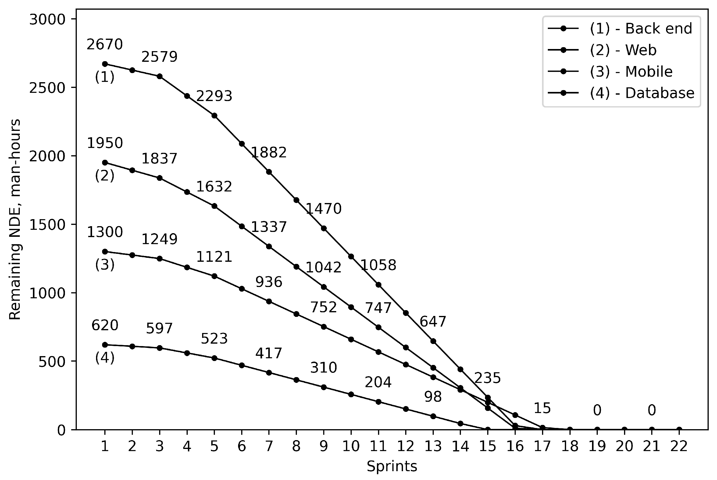
Applying criteria (18) and calculating NDC according to (17), we find the project duration for the optimistic and pessimistic scenarios. In the case of the optimistic scenario, it is going to take 19 sprints (approximately 9.5 months) to implement the project. In turn, for the pessimistic scenario, the project duration is 22 sprints (approximately 11 months). Figure 1 and Figure 2 depict the dynamics of project scope implementation expressed as reduction of NDEs for the remaining project scope (without compromising representation of the general trend, some of the NDE values are omitted intentionally in order to ensure readability of the charts).
The calculations in this section were performed by means of the Google Colab Notebooks technology using Python 3.7.13 as a programming language and the Matplotlib 3.2.2 library for visualization (the used distributions of Python and Matplotlib were provided by the Google Colab as of 9 May 2022).
4. Discussion
4.1. Main Findings
One of the primary outcomes of the current study is the approach to measuring project scope and, consequently, the productivity of a development team. The approach involves using an NDE, which expresses the amount of development efforts in time-based units (e.g., man-hours). Such an approach eliminates a weakness of the “point”-based measurement [3,8,15,16]—the necessity to transform “points” to working time which, in turn, relies on previously accumulated historical data. Instead, NDEs are received as the result of expert judgment (see step 1 of the method).
Proposed in the study the system of working time balance Equation (11) (and its modification (14)), on the one hand, establishes the connection between NDEs and the working time structure of a software developer and, on the other hand, maps working time on a project timeline. In the context of the proposed method, one of the main uses of the system is the expression for NDC of a Scrum team (17).
Based on the idea of NDE and the system of working time balance equations, the method of project duration estimation produces valuable outputs on each of the four steps (1—NDEs, 2—development team composition, 3—release plan, 4—estimated project duration) supposed to be used to inform project stakeholders about the resources and time required to complete the project. In order to minimize the efforts spent on the estimation itself, the method tolerates certain simplifications, in particular, omitting analysis of dependencies between project tasks and reducing risk management to estimating optimistic and pessimistic scenarios only without identification of concrete risks. It is worth noting that due to these simplifications, outputs of the methods are not recommended to be treated as commitments (e.g., when signing a contract with the client).
4.2. Implications for Software Development Lifecycle
One of the common mistakes is doing “one-time” estimation before project implementation starts and using that estimate when making commitments. The main problems with such “one-time” estimates are their low quality (e.g., inappropriate accuracy) as well as difficulties (or even impossibility) in comparing them with the actually spent efforts in the project implementation phase. At the same time, the preparation of such estimates may require a significant amount of effort.
To eliminate the highlighted above problems, it is proposed to consider estimation as an integral part of the software development lifecycle (SDLC). In other words, the estimation is envisioned as a consecutive process, that starts from the very beginning and lasts until the finalization of a project, where outputs of one step are inputs for the next ones. Of course, depending on the SDLC stage, estimation has different goals and requirements for accuracy. The authors have identified five estimation stages summarized in Table 5.
The method introduced in the current study is supposed to be applied in the intermediate estimation stage consuming as inputs results of the preliminary estimation (if any) and providing its outputs to the next stage where the estimate is made definite enough to make commitments. As a result of such a sequential approach, on the one hand, the estimate is gradually refined as the level of uncertainty decreases, and the understanding of the project becomes deeper; on the other hand, the efforts spent on the estimation itself are distributed among the stages giving more flexibility with balancing the load on the team members involved into the estimation process.
In the current form, the proposed estimation technique is applicable for a Scrum-based development process. In the authors’ opinion, the method could also be applied to other Agile methodologies (e.g., Kanban) without significant modifications. If a software development project consists of several iterations, it is recommended that the method is applied to each iteration separately (such an approach is going to ensure better granularity of the estimates). Since the method is going to be used in the intermediate estimate stage, for example, in the early pre-sale stage, the main potential users of the method are software architects involved in the pre-sale process.
4.3. Threats to Validity
As shown in the sections above, the estimated project duration is influenced by the NDC of a Scrum team. However, in practice, it might take place in situations when there are strong dependencies either between project tasks inside a project or on external factors which are out of the project control (e.g., the necessity to wait while another team completes its work). In such cases, the duration of a project is defined rather by the dependencies than the capacity of a team. Therefore, the method is not applicable in such scenarios. It is recommended using, for example, CPM [2] instead.
4.4. Potential Software Automation
The proposed estimation method is simple enough for a cheap ad-hoc implementation by means of spreadsheets (e.g., MS Excel). However, covering all the estimation stages from Table 5 becomes possible only in a full-scaled software product. An example of a concept of such product is provided in [10] where estimation is viewed as a semi-structured [36] and knowledge-intensive [37] business process. Importantly, implementation as a software product allows the accumulation of historical data that, in turn, allow improvements in the estimation process by applying data science techniques. Additionally, integration with issue tracking systems (e.g., Atlassian Jira, Azure DevOps, etc.) is envisioned as a quite useful feature that opens the possibility of automation of collecting feedback on estimates and comparing them with actually spent efforts.
4.5. Limitations and Future Research
One of the outstanding limitations of the method is the impossibility to deal with development teams with mixed specializations (when a particular team member can do tasks from more than one specialization). In the current version, this limitation can be covered by the workaround when a developer with mixed specializations is “virtually” split into two or more developers with partial involvement (e.g., if a full stack engineer can do front-end and back-end tasks, two developers are added to the team composition with 50% of involvement each).
Currently, the method covers one of the most widespread Agile methodologies—Scrum. However, at the persuasion of the authors, with relatively small research efforts, the method can also be adapted to Kanban-based development processes.
It is worth emphasizing the weaknesses of the method such as the absence of guidance on how to choose GPAC and SDAC in step 2. This can be eliminated in two iterations: (1) provide textual instructions to method users that explain the meaning of these coefficients for the users; (2) when enough historical data are collected, apply statistics-based recommendations (of course, this is possible in case of implementation within a full-scaled software product). In particular, the efforts required for defect fixing (which is reflected in GPAC and SDAC) can potentially be evaluated from the software durability perspective [38,39].
The risk management approach included in the current version of the method involves estimation of the optimistic and pessimistic scenarios. However, it is worth considering adding the analysis of explicitly identified risks and evaluating their impact on the estimates [9,40].
Another interesting possibility that can supplement the method is automated recommendations on a development team (in the current version, a team is composed manually in step 3). Such a feature can allow to decrease the amount of manual efforts and accelerate decision-making when “playing” with different potential project implementation scenarios.
One of the promising directions of future research is creating a method of collecting feedback on estimates on the project implementation stage comparing them with actually spent efforts and adjusting estimates of the remaining work. On the one hand, this monitoring method might highlight the areas that require improvements in the proposed estimation method. On the other hand, it unlocks the possibility of collecting historical data that, in turn, lay the foundation for potential usage of machine learning techniques.
5. Conclusions
The goal of the study has been achieved—we have created a method intended for estimating the duration of software development projects supposed to be implemented by scrum teams with differentiated specializations. The method is based on the system of equations reflecting the structure of software developers’ working time. We also proposed an approach to unify the measurement of software developer productivity by introducing the term “average” software developer (ASD) as well as related terms such as normalized development estimate (NDE), normalized development capacity (NDC), and others.
Since the outcomes of the method are not definite enough, they are not recommended to be used for commitments (e.g., on signing a contract with the client). Instead, the outcomes can be used as inputs on the next estimate stage—precise estimation and release planning which, in turn, is supposed to provide outputs reliable enough to make commitments.
From the advantages of the method, it is worth highlighting the following: the system of equations reflecting the structure of software developer working time significantly simplifies further monitoring of project implementation and collection feedback on the estimates; the current version of the method does not require any historical data; relative ease of software automation that allows even spreadsheet-based implementation. The main disadvantages of the method are strong dependency on expert evaluations in step 1 (which is the most effort-intense in comparison to the other steps); lack of definite recommendations on how to choose such parameters as GPACs and SDACs; no automation for recommending a team composition on step 3.
The following steps to evolve the method are envisioned: the creation of the modification intended for Scrum teams with mixed specializations (when a software developer can perform tasks of more than one specialization); automate recommending an optimal team composition that allows reducing manual efforts on step 3; include management of dependencies, assumptions, and risks as significant factors that influence the project duration. It is also important to define a business process that involves application of the method in practice which, in turn, opens an opportunity for its implementation as a part of a full-scale software product (one of the possible concepts is provided in [10]).
Author Contributions
Conceptualization, V.T. and V.V.; Investigation, A.B. and V.V.; Methodology, V.V.; Project administration, V.T. and A.B.; Software, V.V.; Validation, V.T. and A.B.; Visualization, V.V.; Writing—original draft, V.T. and V.V.; Writing—review and editing, V.T. and V.V. All authors have read and agreed to the published version of the manuscript.
Funding
This research received no external funding.
Institutional Review Board Statement
Not applicable.
Informed Consent Statement
Not applicable.
Data Availability Statement
Not applicable.
Acknowledgments
The authors would like to appreciate the editors and the anonymous reviewers for their insightful suggestions to improve the quality of this paper.
Conflicts of Interest
The authors declare no conflict of interest.
Abbreviations
The following abbreviations are used in this manuscript:
| ASD | “Average” software developer |
| CAEA | Constructive agile estimation algorithm |
| CLPC | Competency level productivity coefficient |
| COCOMO | Constructive cost model |
| CPM | Critical path method |
| DWT | Development working time |
| FPA | Functional point analysis |
| GERT | Graphical evaluation and review technique |
| GPAC | General project activities coefficient |
| IPC | Involvement productivity coefficient |
| NDC | Normalized development capacity |
| NDE | Normalized development estimate |
| NDWT | Normalized development working time |
| PC | Productivity coefficient |
| PERT | Program evaluation and review technique |
| SLIM | Software lifecycle management |
| SNAP | Non-functional assessment process |
| SDAC | Supplementary development activities coefficient |
| SDLC | Software development lifecycle |
| UAT | User acceptance testing |
| UCP | Use case point analysis |
References
- Bureau of Naval Weapons, United States, Special Projects Office. Program Evaluation Research Task PERT Summary Report: Phase 1; Special Projects Office, Bureau of Naval Weapons, Department of the Navy: Monterey, CA, USA, 1958. [Google Scholar]
- Kelley, J.E.; Walker, M.R. Critical-Path Planning and Scheduling. In Proceedings of the Eastern Joint IRE-AIEE-ACM Computer Conference, Boston, MA, USA, 1–3 December 1959; Association for Computing Machinery: New York, NY, USA, 1959; pp. 160–173. [Google Scholar] [CrossRef]
- Albrecht, A.J. Measuring Application Development Productivity. In Proceedings of the IBM Applications Development Symposium, Monterey, CA, USA, 14–17 October 1979; IBM Corporation: White Plains, NY, USA, 1979. [Google Scholar]
- Boehm, B.W. Software Engineering Economics; Prentice-Hall: Hoboken, NJ, USA, 1981. [Google Scholar]
- Boehm, B.W. Software Engineering Economics. IEEE Trans. Softw. Eng. 1984, SE-10, 4–21. [Google Scholar] [CrossRef]
- Boehm, B.W.; Abts, C.; Clark, B.K.; Devnani-Chulani, S.; Horowitz, E.; Madachy, R.J.; Reifer, D.J.; Steece, B. COCOMO II Model Definition Manual, Version 2.1; Center for Software Engineering, The University of Southern California: Los Angeles, CA, USA, 1995. [Google Scholar]
- Boehm, B.W.; Abts, C.; Brown, A.W.; Devnani-Chulani, S.; Clark, B.K.; Horowitz, E.; Madachy, R.J.; Reifer, D.J.; Steece, B. Software Cost Estimation with COCOMO II; Prentice-Hall: Hoboken, NJ, USA, 2000. [Google Scholar]
- Grenning, J.W. Planning Poker or How to Avoid Analysis Paralysis While Release Planning. Hawthorn Woods Renaiss. Softw. Consult. 2002, 3, 22–23. [Google Scholar]
- Project Management Institute. Project Management Institute, A Guide To The Project Management Body Of Knowledge (PMBOK-Guide), 6th ed.; PMBOK® Guide; Project Management Institute: Pennsylvania, PA, USA, 2017. [Google Scholar]
- Batyuk, A.; Voityshyn, V. Process Mining-Based Information Technology for Operational Support of Software Projects Estimation. In Proceedings of the XVI International Scientific Conference on Intellectual Systems of Decision-Making and Problems of Computational Intelligence (ISDMCI’2020), Gliwice, Poland, 12–13 May 2020; pp. 9–11. [Google Scholar]
- Pritsker, A.A.B. GERT: Graphical Evaluation and Review Technique; RM-4973-NASA; Rand Corp.: Santa Monica, CA, USA, 1966. [Google Scholar]
- Putnam, L.H. A General Empirical Solution to the Macro Software Sizing and Estimating Problem. IIEEE Trans. Softw. Eng. 1978, SE-4, 345–361. [Google Scholar] [CrossRef]
- Putnam, L.H.; Myers, W. Measures for Excellence: Reliable Software on Time, Within Budget; Yourdon Press: New York, NY, USA, 1992. [Google Scholar]
- Ghafory, H.; Sahnosh, F.A. The Review of Software Cost Estimation Model: SLIM. Int. J. Adv. Acad. Stud. 2020, 2, 511–515. [Google Scholar]
- Karner, G. Resource Estimation for Objectory Projects. Object. Syst. SF AB 1993, 17, 9. [Google Scholar]
- Tichenor, C. A New Software Metric to Complement Function Points: The Software Non-Functional Assessment Process (SNAP). CrossTalk J. 2013, 26, 21–26. [Google Scholar]
- Mallidi, R.K.; Sharma, M. Study on Agile Story Point Estimation Techniques and Challenges. Int. J. Comput. Appl. 2021, 174, 9–14. [Google Scholar] [CrossRef]
- Coelho, E.; Basu, A. Effort Estimation in Agile Software Development Using Story Points. Int. J. Appl. Inf. Syst. 2012, 3, 7–10. [Google Scholar] [CrossRef]
- Munialo, S.W.; Muketha, G.M. A Review of Agile Software Effort Estimation Methods. Int. J. Comput. Appl. Technol. Res. 2016, 5, 612–618. [Google Scholar] [CrossRef]
- Bhalerao, S.; Ingle, M. Incorporating Vital Factors in Agile Estimation through Algorithmic Method. Int. J. Comput. Sci. Appl. 2009, 6, 85–97. [Google Scholar]
- Alshammari, F.H. Cost Estimate in Scrum Project with the Decision-Based Effort Estimation Technique. Soft Comput. 2022. [Google Scholar] [CrossRef]
- Sudarmaningtyas, P.; Mohamed, R. A Review Article on Software Effort Estimation in Agile Methodology. Pertanika J. Sci. Technol. 2021, 29, 837–861. [Google Scholar] [CrossRef]
- Usman, M.; Mendes, E.; Weidt, F.; Britto, R. Effort Estimation in Agile Software Development: A Systematic Literature Review. In Proceedings of the 10th International Conference on Predictive Models in Software Engineering, Turin, Italy, 17 September 2014; pp. 82–91. [Google Scholar] [CrossRef]
- Saeed, A.; Butt, W.H.; Kazmi, F.; Arif, M. Survey of Software Development Effort Estimation Techniques. In Proceedings of the 2018 7th International Conference on Software and Computer Applications (ICSCA 2018), Kuantan, Malaysia, 8–10 February 2018; Association for Computing Machinery: New York, NY, USA, 2018; pp. 82–86. [Google Scholar] [CrossRef]
- Vyas, M.; Bohra, A.; Lamba, D.C.S.; Vyas, A. A Review on Software Cost and Effort Estimation Techniques for Agile Development Process. Int. J. Recent Res. Asp. 2018, 5, 1–5. [Google Scholar]
- Habibi, F.; Birgani, O.T.; Koppelaar, H.; Radenović, S.N. Using Fuzzy Logic to Improve the Project Time and Cost Estimation Based on Project Evaluation and Review Technique (PERT). J. Proj. Manag. 2018, 3, 183–196. [Google Scholar] [CrossRef]
- Nassif, A.B.; Azzeh, M.; Idri, A.; Abran, A. Software Development Effort Estimation Using Regression Fuzzy Models. Comput. Intell. Neurosci. 2019, 2019, 8367214. [Google Scholar] [CrossRef] [PubMed]
- van Dorp, J.R. A Dependent Project Evaluation and Review Technique: A Bayesian Network Approach. Eur. J. Oper. Res. 2020, 280, 689–706. [Google Scholar] [CrossRef]
- Shabeer, M.K.P.; Krishnan, S.I.U.; Deepa, G. Software Effort Estimation Using Genetic Algorithms with the Variance-Accounted-for (VAF) and the Manhattan Distance. In Ubiquitous Intelligent Systems; Smart Innovation, Systems and Technologies; Karuppusamy, P., Perikos, I., García Márquez, F.P., Eds.; Springer: Singapore, 2021; Volume 243, pp. 421–434. [Google Scholar] [CrossRef]
- Satapathy, S.M.; Acharya, B.P.; Rath, S.K. Early Stage Software Effort Estimation Using Random Forest Technique Based on Use Case Points. Inst. Eng. Technol. Softw. 2016, 10, 10–17. [Google Scholar] [CrossRef]
- Mahmood, Y.; Kama, N.; Azmi, A.; Khan, A.S.; Ali, M. Software Effort Estimation Accuracy Prediction of Machine Learning Techniques: A Systematic Performance Evaluation. J. Softw. Pract. Exp. 2021, 52, 39–65. [Google Scholar] [CrossRef]
- Trendowicz, A.; Jeffery, R. Classification of Effort Estimation Methods. In Software Project Effort Estimation; Springer: Cham, Switzerland, 2014; pp. 155–208. [Google Scholar] [CrossRef]
- Zarour, A.; Zein, S. Software Development Estimation Techniques in Industrial Contexts: An Exploratory Multiple Case-Study. Int. J. Technol. Educ. Sci. 2019, 3, 72–84. [Google Scholar]
- Boehm, B.; Abts, C.; Chulani, S. Software Development Cost Estimation Approaches—A Survey. Ann. Softw. Eng. 2000, 10, 177–205. [Google Scholar] [CrossRef]
- Tuckman, B.W. Developmental Sequence in Small Groups. Psychol. Bull. 1965, 63, 384–399. [Google Scholar] [CrossRef] [PubMed]
- van der Aalst, W.M.P. Process Mining: Data Science in Action, 2nd ed.; Springer: Berlin, Germany, 2016. [Google Scholar] [CrossRef]
- Di Ciccio, C.; Marrella, A.; Russo, A. Knowledge-Intensive Processes: Characteristics, Requirements and Analysis of Contemporary Approaches. J. Data Semant. 2015, 4, 29–57. [Google Scholar] [CrossRef]
- Kumar, R.; Khan, S.A.; Khan, R.A. Durability Challenges in Software Engineering. J. Def. Softw. Eng. 2016, 42, 29–31. [Google Scholar]
- Khan, S.A.; Alenezi, M.; Agrawal, A.; Kumar, R.; Khan, R.A. Evaluating Performance of Software Durability through an Integrated Fuzzy-Based Symmetrical Method of ANP and TOPSIS. Symmetry 2020, 12, 493. [Google Scholar] [CrossRef]
- Sahu, K.; Shree, R.; Kumar, R. Risk Management Perspective in SDLC. Int. J. Adv. Res. Comput. Sci. Softw. Eng. 2014, 4, 1247–1251. [Google Scholar]
Figure 1.
The dynamics of remaining NDE reduction for the optimistic scenario.
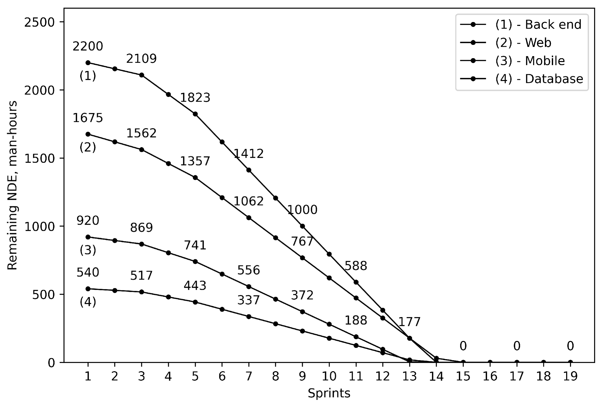
Figure 2.
The dynamics of remaining NDE reduction for the pessimistic scenario.

Table 1.
Estimation methods overview.
| No. | Estimation Method | Abbreviation | Category 1 | SDLC Stage 2 | Basic Measure Unit 3 | Usage of Historical Data | Relying on Expert Judgement |
|---|---|---|---|---|---|---|---|
| 1 | Project evaluation and review technique | PERT | Expertise-based | Analysis and design (ending), implementation | Man-hour | No | Yes |
| 2 | Critial path method | CPM | Expertise-based | Analysis and design (ending), implementation | Man-hour | No | Yes |
| 3 | Graphical evaluation and review technique | GERT | Expertise-based | Analysis and design (ending), implementation | Man-hour | No | Yes |
| 4 | Software lifecycle management | SLIM | Model-based | Analysis and design | Effective LOC | Yes | No |
| 5 | Functional point analysis | FPA | Model-based | Analysis and design | Function point | Yes | No |
| 6 | Use case point analysis | UCP | Model-based | Analysis and design | Use case point | Yes | No |
| 7 | Software non-functional assessment process | SNAP | Model-based | Analysis and design | SNAP point | Yes | No |
| 8 | Constructive cost model | COCOMO | Model-based | Analysis and design | LOC | Yes | No |
| 9 | Constructive cost model II | COCOMO II | Composite | Analysis and design | LOC, function point, use case point | Yes | Yes 4 |
| 10 | Planning poker and its modifications | n/a | Expertise-based | Implementation | Story point | No | Yes |
| 11 | Constructive Agile Estimation Algorithm | CAEA | Model-based, Expertise-based | Analysis and Design, Implementation | Story point | Yes | Yes |
| 12 | Estimation of project duration for Scrum team with differentiated specializations | n/a | Expertise-based | Analysis and design (beginning) | Man-hour | No | Yes |
1 It is applied classification of the estimation methods from [34]. 2 The SDLC stages are taken from Table 5. 3 Basic measure unit is a measurement unit used to size software. 4 In COCOMO II, expert opinion can be used if historical data are not available.
Table 2.
Optimistic and pessimistic NDEs.
| Specialization Identifier, s | Specialization Name | , Man-Hours | , Man-Hours |
|---|---|---|---|
| 1 | Back end | 2200 | 2670 |
| 2 | Web | 1675 | 1950 |
| 3 | Mobile | 920 | 1300 |
| 4 | Database | 540 | 620 |
Table 3.
Project release plan.
| Phase Identifier, p | Phase Name | Total Number of Sprints | Number of Mandatory Sprints 1 | , Hours 2 | Development Team | |||
|---|---|---|---|---|---|---|---|---|
| a | Project start | 2 | 2 | 152 | Core team | 0.50 | 0.40 | 1 |
| b | Team scaling | 2 | 0 | 152 | Whole team | 0.40 | 0.35 | 1 |
| c | Performing | 0 | Whole team | 0.20 | 0.25 | 1 | ||
| d | Stabilization | 1 | 1 | 76 | Whole team | 1.00 | n/a | 0 |
| e | UAT | 2 | 2 | 152 | Reduced team | 1.00 | n/a | 0 |
| f | Releasing | 2 | 2 | 152 | Reduced team | 1.00 | n/a | 0 |
1 The project release plan defines 7 mandatory sprints: 2 sprints on phase a, 1 sprint on phase d, 2 sprints on phases e and f respectively. The number of the other sprints varies depending on the estimated amount of project scope. 2 Duration of each sprint is 2 weeks which is 10 working days or 80 working hours. Assuming that, on average, for each month, there is 1 state holiday; consequently, every 2 sprints miss 1 working day or 8 working hours. Hence, the duration of a project sprint is 76 (not 80) working hours.
Table 4.
Development team composition.
| Software Developer Identifier, j | Project Role | Competency Level | s | 1 | ||||||
|---|---|---|---|---|---|---|---|---|---|---|
| 1 | Technical leader and back-end engineer | Senior | 1 | 1.2 | 0.5 | 0.5 | 0.50 | 0.50 | 0.5 | 0.5 |
| 2 | Back-end engineer | Senior | 1 | 1.2 | 1 | 1 | 1 | 1 | 0 | 0 |
| 3 | Back-end engineer | Middle | 1 | 1 | 1 | 1 | 1 | 1 | 1 | 1 |
| 4 | Back-end engineer | Middle | 1 | 1 | 1 | 1 | 1 | 1 | 0 | 0 |
| 5 | Back-end engineer | Junior | 1 | 0.7 | 1 | 1 | 1 | 1 | 1 | 1 |
| 6 | Front-end engineer | Senior | 2 | 1.2 | 1 | 1 | 1 | 1 | 0 | 0 |
| 7 | Front-end engineer | Middle | 2 | 1 | 1 | 1 | 1 | 1 | 1 | 1 |
| 8 | Front-end engineer | Middle | 2 | 1 | 1 | 1 | 1 | 1 | 1 | 1 |
| 9 | Mobile engineer | Middle | 3 | 1 | 1 | 1 | 1 | 1 | 1 | 1 |
| 10 | Mobile engineer | Middle | 3 | 1 | 1 | 1 | 1 | 1 | 0 | 0 |
| 11 | Database engineer | Senior | 4 | 1.2 | 0.5 | 0.5 | 0.50 | 0.50 | 0.5 | 0.5 |
| 12 | Database engineer | Junior | 4 | 0.7 | 1 | 1 | 1 | 1 | 0 | 0 |
1 Engineers participating in the development team have differentiated specializations, i.e., a particular developer has only one specialization and cannot perform tasks of the other specializations which is reflected in the CLPC.
Table 5.
Estimation in the context of SDLC.
| No. | Estimation Stage | Estimation Goals | Estimate Accuracy 1 | Using Estimates for Commitments | SDLC Stage |
|---|---|---|---|---|---|
| 1 | Preliminary estimation | Roughly understand the required resources and timeline | Very low accuracy | Strictly not recommended | Ideation |
| 2 | Intermediate estimation | Provide more accurate estimates than on the previous stage | Low accuracy | Not recommended | Analysis and design (beginning) |
| 3 | Precise estimation and release planning | Prepare definite estimates [9] and detailed release plan | Acceptable accuracy | Can be recommended | Analysis and design (ending) |
| 4 | Implementation monitoring | Compare estimates with actually spent efforts and clarify remaining estimates | Continuously adjusting accuracy | Can be recommended | Implementation |
| 5 | Finalizing feedback on estimates | Finalize feedback on estimates | n/a | n/a | Finalization |
1 Under the estimate accuracy, it is understood that the closeness of the estimates to the corresponding actually spent efforts; of course, the accuracy defined in this way can be measured only on the project implementation phase.
Publisher’s Note: MDPI stays neutral with regard to jurisdictional claims in published maps and institutional affiliations. |
© 2022 by the authors. Licensee MDPI, Basel, Switzerland. This article is an open access article distributed under the terms and conditions of the Creative Commons Attribution (CC BY) license (https://creativecommons.org/licenses/by/4.0/).
Share and Cite
MDPI and ACS Style
Teslyuk, V.; Batyuk, A.; Voityshyn, V. Method of Software Development Project Duration Estimation for Scrum Teams with Differentiated Specializations. Systems 2022, 10, 123. https://doi.org/10.3390/systems10040123
AMA Style
Teslyuk V, Batyuk A, Voityshyn V. Method of Software Development Project Duration Estimation for Scrum Teams with Differentiated Specializations. Systems. 2022; 10(4):123. https://doi.org/10.3390/systems10040123
Chicago/Turabian StyleTeslyuk, Vasyl, Anatoliy Batyuk, and Volodymyr Voityshyn. 2022. "Method of Software Development Project Duration Estimation for Scrum Teams with Differentiated Specializations" Systems 10, no. 4: 123. https://doi.org/10.3390/systems10040123
Note that from the first issue of 2016, this journal uses article numbers instead of page numbers. See further details here.