
Quantifying Mosaic Development: Towards an Evo-Devo Postmodern Synthesis of the Evolution of Development via Differentiation Trees of Embryos

Abstract
:1. Introduction
Higher-Order Patterns and Organization by Differentiation
2. Materials and Methods
2.1. Description of Datasets, Ciona Intestinalis
2.2. Description of Datasets, Caenorhabditis elegans
2.3. Methods for Collecting Secondary Data
2.4. Finding Biologically-Meaningful Asymmetric Divisions
2.5. Ratio Between Larger and Smaller Daughter Cells
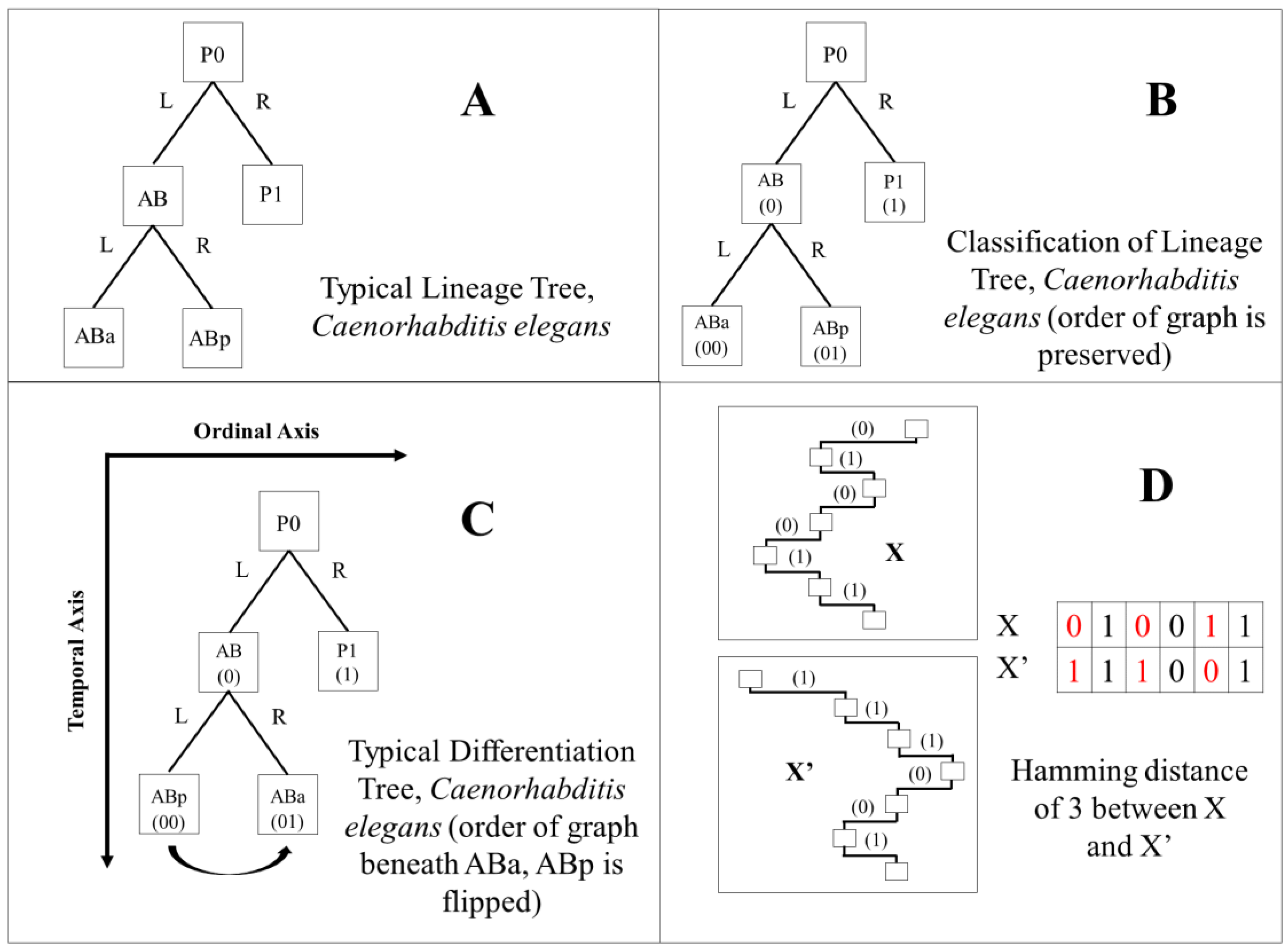
2.6. Differentiation Trees
2.7. Differentiation Code and Tree Classification
2.8. Composite Differentiation Code
2.9. Power Regression Formula
2.10. Hamming Distance Calculation
2.11. Three-Dimensional Representation of Hamming Distances in C. elegans
2.12. CAST (Cell Alignment Search Tool) Analysis
2.13. Graphs and Analysis
3. Results
3.1. Introduction to Analysis
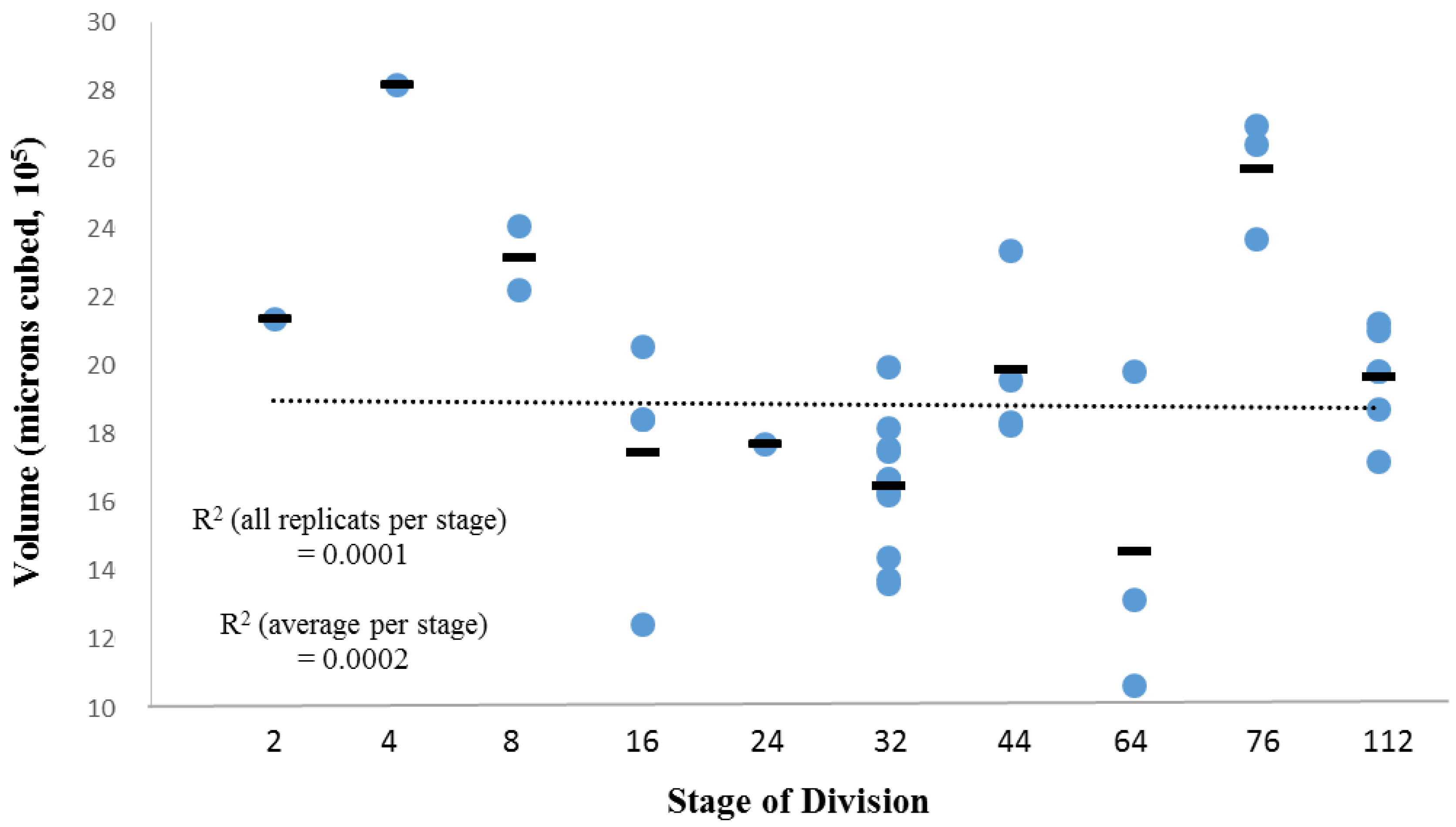
3.2. Within-Species Embryonic Variation
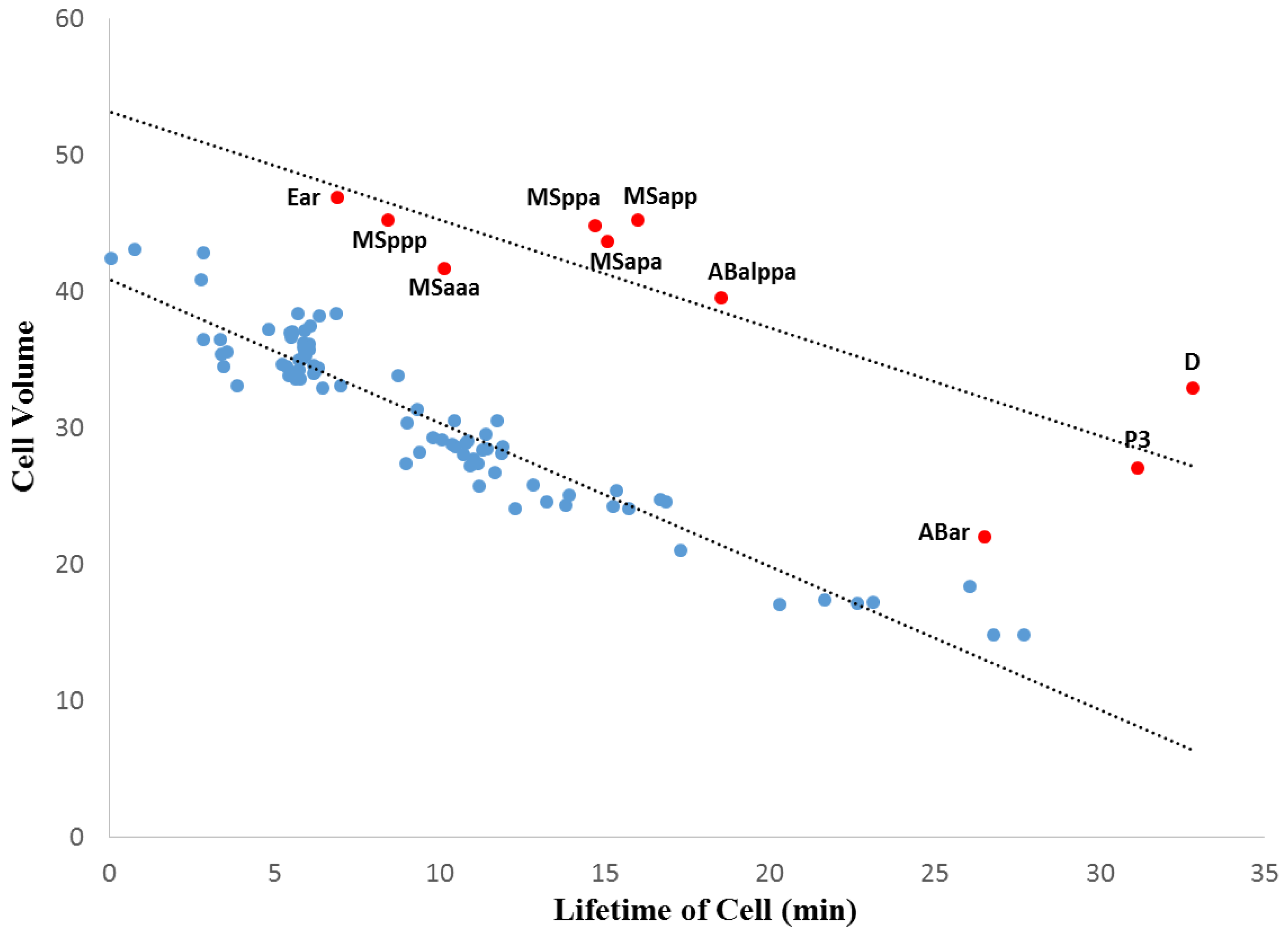
3.3. Cellular Variation Across Lineage Trees
3.4. Comparison of Lineage and Differentiation Trees
3.5. Intra-Specific Comparisons Using Isometric Graphs
3.6. CAST Analysis of Differentiation Codes
3.7. Interpretation of Results
4. Discussion
4.1. Analytical Caveats
4.2. Discussion of Within-Species Cellular Variation
4.3. Differentiation Trees and Comparative Development
4.4. Overarching Features of Mosaic Embryogenesis
4.5. Broader Evolutionary Implications
4.6. A Toy Model of an Idealized Mosaic Embryo
5. Conclusions
Supplementary Materials
Acknowledgments
Author Contributions
Conflicts of Interest
References
- Driesch, H.A.E. The potency of the first two cleavage cells in the development of echinoderms [translation of 1891 German version]. In Great Experiments in Biology; Gabriel, M., Fogel, S., Eds.; Prentice-Hall: Englewoods Cliffs, NJ, USA, 1955; pp. 210–214. [Google Scholar]
- Wilson, E.B. Experimental studies in germinal localization: II. Experiments on the cleavage-mosaic in Patella and Dentalium. J. Exp. Zool. 1904, 1, 197–268. [Google Scholar] [CrossRef]
- Lawrence, P.A.; Levine, M. Mosaic and regulative development: Two faces of one coin. Curr. Biol. 2006, 16, R236–R239. [Google Scholar] [CrossRef] [PubMed]
- Waddington, C.H. Principles of Embryology; George Allen & Unwin Ltd.: London, UK, 1956. [Google Scholar]
- Vogt, W. Mosaikcharakter und Regulation in der Frühentwicklung des Amphibieneies. Verh. Dtsch. Zool. Ges. 1928, 32, 26–70. (In German) [Google Scholar]
- McCain, E.R.; Cather, J.N. Regulative and mosaic development of Ilyanassa obsoleta embryos lacking the A and C quadrants. Invertebr. Reprod. Dev. 1989, 15, 185–192. [Google Scholar] [CrossRef]
- Cunha, A.; Azevedo, R.B.R.; Emmons, S.W.; Leroi, A.M. Developmental biology: Variable cell number in nematodes. Nature 1999, 402, 253–253. [Google Scholar] [PubMed]
- Nishida, H.; Stach, T. Cell lineages and fate maps in tunicates: Conservation and modification. Zool. Sci. 2014, 31, 645–652. [Google Scholar] [CrossRef] [PubMed]
- Meinertzhagen, I.A. Eutely, cell lineage, and fate within the ascidian larval nervous system: Determinacy or to be determined? Can. J. Zool. 2005, 83, 184–195. [Google Scholar] [CrossRef]
- Gordon, N.K.; Gordon, R. Embryogenesis Explained; World Scientific Publishing Company: Singapore, 2016. [Google Scholar]
- Rochlin, K.; Yu, S.; Roy, S.; Baylies, M.K. Myoblast fusion: When it takes more to make one. Dev. Biol. 2010, 341, 66–83. [Google Scholar] [CrossRef] [PubMed]
- Idema, T.; Dubuis, J.O.; Kang, L.; Manning, M.L.; Nelson, P.C.; Lubensky, T.C.; Liu, A.J. The syncytial Drosophila embryo as a mechanically excitable medium. PLoS ONE 2013, 8, e77216. [Google Scholar]
- Gordon, R. The Hierarchical Genome and Differentiation Waves: Novel Unification of Development, Genetics and Evolution; World Scientific & Imperial College Press: Singapore; London, UK, 1999. [Google Scholar]
- Gordon, N.K.; Gordon, R. The organelle of differentiation in embryos: The cell state splitter. Theor. Biol. Med. Model. 2016. [Google Scholar] [CrossRef] [PubMed]
- Essam, J.W.; Fisher, M.E. Some basic definitions in graph theory. Rev. Mod. Phys. 1970, 42, 272–288. [Google Scholar] [CrossRef]
- Gordon, R. On Monte Carlo algebra. J. Appl. Probab. 1970, 7, 373–387. [Google Scholar] [CrossRef]
- Wang, L. Directed Acyclic Graph. In Encyclopedia of Systems Biology; Dubitsky, W., Wolkenhauer, O., Cho, K.-H., Yokota, H., Eds.; Springer: Berlin, Germany, 2013; p. 574. [Google Scholar]
- Wikipedia Planar Graph. Available online: https://en.wikipedia.org/wiki/Planar_graph (accessed on 28 March 2016).
- Bonichon, N.; Gavoille, C.; Hanusse, N.; Poulalhon, D.; Schaeffer, G. Planar graphs, via well-orderly maps and trees. Graphs Comb. 2006, 22, 185–202. [Google Scholar] [CrossRef]
- Riordan, J. The numbers of labeled colored and chromatic trees. Acta Math. 1957, 97, 211–225. [Google Scholar] [CrossRef]
- Jacobson, G. Space-efficient static trees and graphs. In Proceedings of the 30th Annual Symposium on Foundations of Computer Science, Research Triangle Park, NC, USA, 30 October–1 November 1989; pp. 549–554.
- Crescenzi, P.; Penna, P. Strictly-upward drawings of ordered search trees. Theor. Comput. Sci. 1998, 203, 51–67. [Google Scholar] [CrossRef]
- Di Battista, G.; Eades, P.; Tamassia, R.; Tollis, I.G. Algorithms for drawing graphs: An annotated bibliography. Comput. Geom. Theory Appl. 1994, 4, 235–282. [Google Scholar] [CrossRef]
- Rusu, A.; Clement, C.; Jianu, R. Adaptive binary trees visualization with respect to user-specified quality measures. Proc. Int. Conf. Inf. Vis. 2006, 10, 469–474. [Google Scholar]
- Garg, A.; Goodrich, M.T.; Tamassia, R. Planar upward tree drawings with optimal area. Int. J. Comput. Geom. Appl. 1996, 6, 333–356. [Google Scholar] [CrossRef]
- Sulston, J.E.; Schierenberg, E.; White, J.G.; Thomson, J.N. The embryonic cell lineage of the nematode Caenorhabditis elegans. Dev. Biol. 1983, 100, 64–119. [Google Scholar] [CrossRef]
- Wikipedia Graph Isomorphism. Available online: https://en.wikipedia.org/wiki/Graph_isomorphism (accessed on 28 March 2016).
- Hedgecock, E.M. Cell lineage mutants in the nematode Caenorhabditis elegans. Trends Neurosci. 1985, 8, 288–293. [Google Scholar] [CrossRef]
- Sternberg, P.W.; Horvitz, H.R. Gonadal cell lineages of the nematode Panagrellus redivivus and implications for evolution by the modification of cell lineage. Dev. Biol. 1981, 88, 147–166. [Google Scholar] [CrossRef]
- Vandenberg, L.N.; Levin, M. A unified model for left-right asymmetry? Comparison and synthesis of molecular models of embryonic laterality. Devel. Biol. 2013, 379, 1–15. [Google Scholar] [CrossRef]
- Goldstein, B. On the evolution of early development in the Nematoda. Philos. Trans. R. Soc. Lond. B Biol. Sci. 2001, 356, 1521–1531. [Google Scholar] [CrossRef] [PubMed]
- Gordon, R. Walking the tightrope: The dilemmas of hierarchical instabilities in Turing’s morphogenesis. In The Once and Future Turing: Computing the World; Cooper, S.B., Hodges, A., Eds.; Cambridge University Press: Cambridge, UK, 2015; pp. 150–164. [Google Scholar]
- Koonin, E.V. Towards a postmodern synthesis of evolutionary biology. Cell Cycle 2009, 8, 799–800. [Google Scholar] [CrossRef] [PubMed]
- Metz, J.A.J. Thoughts on the geometry of meso-evolution: Collecting mathematical elements for a postmodern synthesis. In Mathematics of Darwin's Legacy; Chalub, F.A.C.C., Rodrigues, J.F., Eds.; Springer: Basel, Switzerland, 2011; pp. 193–231. [Google Scholar]
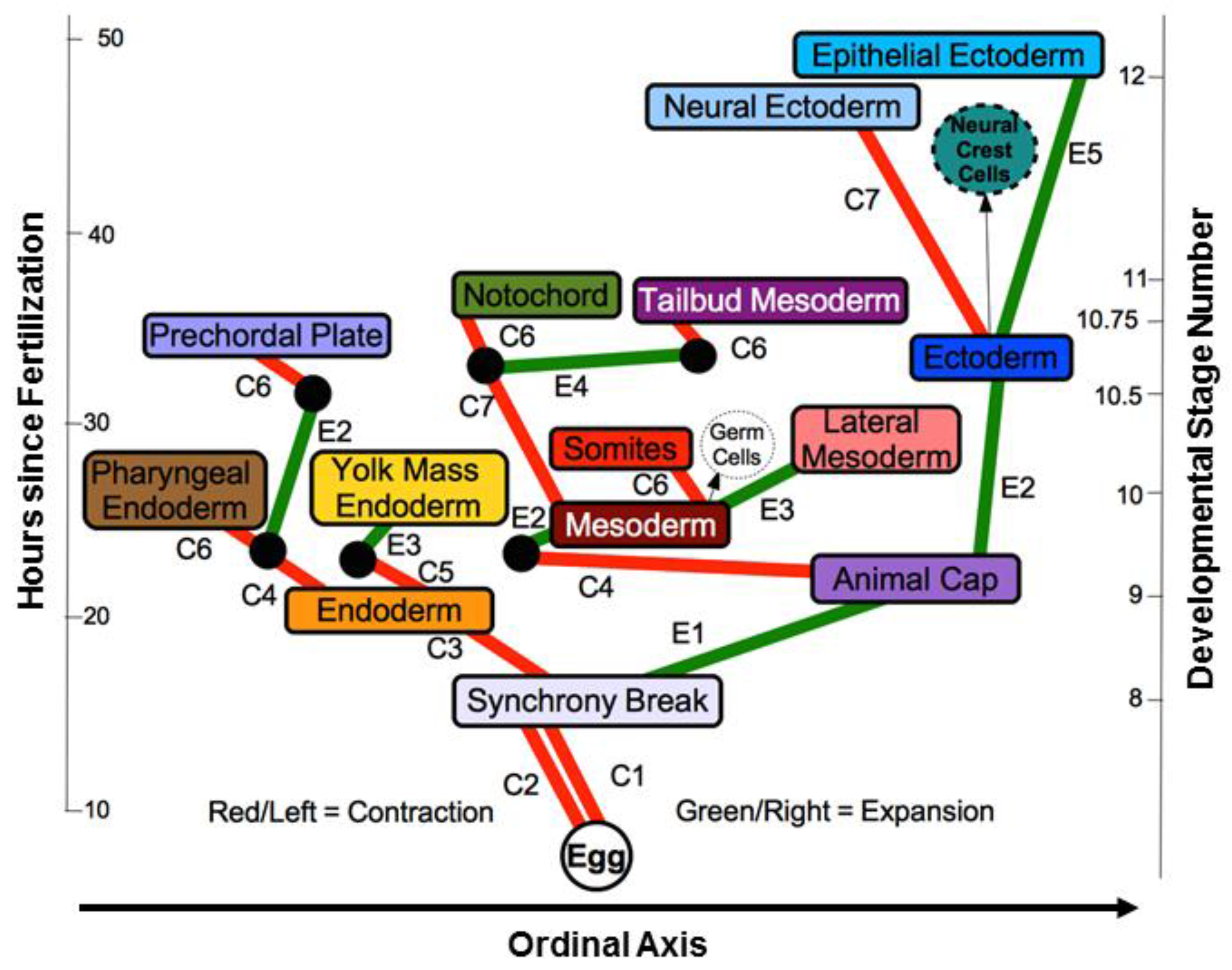
- Björklund, N.K.; Gordon, R. Surface contraction and expansion waves correlated with differentiation in axolotl embryos. I. Prolegomenon and differentiation during the plunge through the blastopore, as shown by the fate map. Comput. Chem. 1994, 18, 333–345. [Google Scholar] [CrossRef]
- Shapiro, E.; Biezuner, T.; Linnarsson, S. Single-cell sequencing-based technologies will revolutionize whole-organism science. Nat. Rev. Genet. 2013, 14, 618–630. [Google Scholar] [CrossRef] [PubMed]
- Veeman, M.; Reeves, W. Quantitative and in toto imaging in ascidians: Working toward an image-centric systems biology of chordate morphogenesis. Genesis 2015, 53, 143–159. [Google Scholar] [CrossRef] [PubMed]
- Stach, T.; Anselmi, C. High-precision morphology: Bifocal 4D-microscopy enables the comparison of detailed cell lineages of two chordate species separated for more than 525 million years. BMC Biol. 2015. [Google Scholar] [CrossRef] [PubMed]
- Hudson, C.; Yasuo, H. Similarity and diversity in mechanisms of muscle fate induction between ascidian species. Biol. Cell 2008, 100, 265–277. [Google Scholar] [CrossRef] [PubMed]
- Wikipedia Synapomorphy. Available online: https://en.wikipedia.org/wiki/Synapomorphy (accessed on 30 March 2016).
- McGhee, G.R. Convergent Evolution: Limited Forms Most Beautiful; MIT Press: Cambridge, MA, USA, 2011. [Google Scholar]
- Bao, Z.R.; Zhao, Z.Y.; Boyle, T.J.; Murray, J.I.; Waterston, R.H. Control of cell cycle timing during C. elegans embryogenesis. Dev. Biol. 2008, 318, 65–72. [Google Scholar] [CrossRef] [PubMed]
- Ho, V.W.; Wong, M.K.; An, X.; Guan, D.; Shao, J.; Ng, H.C.; Ren, X.; He, K.; Liao, J.; Ang, Y.; et al. Systems-level quantification of division timing reveals a common genetic architecture controlling asynchrony and fate asymmetry. Mol. Syst. Biol. 2015. [Google Scholar] [CrossRef] [PubMed]
- Tiraihi, A.; Tiraihi, M.; Tiraihi, T. Self-organization of developing embryo using scale-invariant approach. Theor. Biol. Med. Model. 2011. [Google Scholar] [CrossRef] [PubMed]
- Arata, Y.; Takagi, H.; Sako, Y.; Sawa, H. Power law relationship between cell cycle duration and cell volume in the early embryonic development of Caenorhabditis elegans. Front. Physiol. 2015. [Google Scholar] [CrossRef] [PubMed]
- Ginzberg, M.B.; Kafri, R.; Kirschner, M. On being the right (cell) size. Science 2015. [Google Scholar] [CrossRef] [PubMed]
- Sulston, J.E. C. elegans: The cell lineage and beyond. Biosci. Rep. 2003, 23, 49–66. [Google Scholar] [CrossRef] [PubMed]
- Roubinet, C.; Cabernard, C. Control of Asymmetric cell division. Curr. Opin. Cell Biol. 2014, 31, 84–91. [Google Scholar] [CrossRef] [PubMed]
- Bordzilovskaya, N.P.; Dettlaff, T.A.; Duhon, S.T.; Malacinski, G.M. Developmental-stage series of axolotl embryos [Erratum: Staging Table 19-1 is for 20 °C, not 29 °C]. In Developmental Biology of the Axolotl; Armstrong, J.B., Malacinski, G.M., Eds.; Oxford University Press: New York, NY, USA, 1989; pp. 201–219. [Google Scholar]
- Nieuwkoop, P.D.; Björklund, N.K.; Gordon, R. Surface contraction and expansion waves correlated with differentiation in axolotl embryos. II. In contrast to urodeles, the anuran Xenopus laevis does not show furrowing surface contraction waves. Int. J. Dev. Biol. 1996, 40, 661–664. [Google Scholar] [PubMed]
- Brodland, G.W.; Gordon, R.; Scott, M.J.; Björklund, N.K.; Luchka, K.B.; Martin, C.C.; Matuga, C.; Globus, M.; Vethamany-Globus, S.; Shu, D. Furrowing surface contraction wave coincident with primary neural induction in amphibian embryos. J. Morphol. 1994, 219, 131–142. [Google Scholar] [CrossRef] [PubMed]
- Nakamura, M.J.; Terai, J.; Okubo, R.; Hotta, K.; Oka, K. Three-dimensional anatomy of the Ciona intestinalis tailbud embryo at single-cell resolution. Dev. Biol. 2012, 372, 274–284. [Google Scholar] [CrossRef] [PubMed]
- Tassy, O.; Dauga, D.; Daian, F.; Sobral, D.; Robin, F.; Khoueiry, P.; Salgado, D.; Fox, V.; Caillol, D.; Schiappa, R.; et al. The ANISEED database: Digital representation, formalization, and elucidation of a chordate developmental program. Genome Res. 2010, 20, 1459–1468. [Google Scholar] [CrossRef] [PubMed]
- Aniseed Aniseed Data: C. intestinalis. Available online: http://www.aniseed.cnrs.fr/aniseed/download/download_data (accessed on 28 March 2016).
- Bao, Z.R.; Murray, J.I.; Boyle, T.; Ooi, S.L.; Sandel, M.J.; Waterston, R.H. Automated cell lineage tracing in Caenorhabditis elegans. Proc. Natl. Acad. Sci. USA 2006, 103, 2707–2712. [Google Scholar] [CrossRef] [PubMed]
- Cirino, P.; Toscano, A.; Caramiello, D.; Macina, A.; Miraglia, V.; Monte, A. Laboratory Culture of the Ascidian Ciona intestinalis (L.): A Model System for Molecular Developmental Biology Research. Available online: http://comm.archive.mbl.edu/BiologicalBulletin/MMER/cirino/CirTit.html (accessed on 14 August 2016).
- Bianchi, L.; Driscoll, M. Culture of Embryonic C. elegans Cells for Electrophysiological and Pharmacological Analyses. Available online: http://www.ncbi.nlm.nih.gov/books/NBK19713/ (accessed on 28 March 2016).
- Granville, V. Developing Analytic Talent: Becoming a Data Scientist; Wiley: Hoboken, NJ, USA, 2014. [Google Scholar]
- Wikipedia GIMP. Available online: https://en.wikipedia.org/wiki/GIMP (accessed on 28 March 2016).
- Alicea, B.; Gordon, R. C. intestinalis Embryonic Differentiation Tree (1- to 112-cell stage). Available online: https://figshare.com/articles/C_intestinalis_Embryonic_Differentiation_Tree_1_to_112_cell_stage_/2117152 (accessed on 28 March 2016).
- Alicea, B.; Gordon, R. C. elegans Embryonic Differentiation Tree (10 Division Events). Available online: https://figshare.com/articles/C_elegans_Embryonic_Differentiation_Tree_10_division_events_/2118049 (accessed on 28 March 2016).
- Hobert, O. Neurogenesis in the Nematode Caenorhabditis elegans. Available online: http://www.ncbi.nlm.nih.gov/books/NBK116086/ (accessed on 28 March 2016).
- Hobert, O. Neurogenesis in the nematode Caenorhabditis elegans. In Comprehensive Developmental Neuroscience: Patterning and Cell Type Specification in the Developing Cns and Pns; Rubenstein, J.L.R., Rakic, P., Eds.; Elsevier Academic Press: San Diego, CA, USA, 2013; pp. 609–626. [Google Scholar]
- Goldstein, B.; Hird, S.N.; White, J.G. Cell polarity in early C. elegans development. Development 1993, Supplement, 279–287. [Google Scholar]
- Bhatla, N. C. elegans Cell Lineage. Available online: http://wormweb.org/celllineage#c=P0&z=1 (accessed on 28 March 2016).
- Nishida, H. Cell lineage analysis in ascidian embryos by intracellular injection of a tracer enzyme. III. Up to the tissue restricted stage. Dev. Biol. 1987, 121, 526–541. [Google Scholar] [CrossRef]
- Rose, L.; Gonczy, P. Polarity establishment, asymmetric division and segregation of fate determinants in early C. elegans embryos. WormBook 2014, 1–43. [Google Scholar]
- Packard, G.C. On the use of log-transformation versus nonlinear regression for analyzing biological power laws. Biol. J. Linn. Soc. 2014, 113, 1167–1178. [Google Scholar] [CrossRef]
- Hamming, R.W. Error detecting and error correcting codes. Bell Syst. Tech. J. 1950, 29, 147–160. [Google Scholar] [CrossRef]
- Wikipedia BLAST. Available online: https://en.wikipedia.org/wiki/BLAST (accessed on 28 March 2016).
- Needleman, S.B.; Wunsch, C.D. A general method applicable to the search for similarities in the amino acid sequence of two proteins. J. Mol. Biol. 1970, 48, 443–453. [Google Scholar] [CrossRef]
- Alicea, B.; Portegys, T.; Gordon, R. Information isometry technique reveals organizational features in developmental cell lineages. bioRxiv 2016. [Google Scholar] [CrossRef]
- Bossinger, O.; Schierenberg, E. Early embryonic induction in C. elegans can be inhibited with polysulfated hydrocarbon dyes. Dev. Biol. 1996, 176, 17–21. [Google Scholar] [CrossRef] [PubMed]
- Sternberg, P.W.; Horvitz, H.R. The genetic control of cell lineage during nematode development. Annu. Rev. Genet. 1984, 18, 489–524. [Google Scholar] [CrossRef] [PubMed]
- Lyczak, R.; Gomes, J.E.; Bowerman, B. Heads or tails: Cell polarity and axis formation in the early Caenorhabditis elegans embryo. Dev. Cell 2002, 3, 157–166. [Google Scholar] [CrossRef]
- Banks, K. Thunderbirds, pterosaurs and tumblers: The biomechanics of flight. Harv. Sci. Rev. 2011, 31–33. [Google Scholar]
- Azevedo, R.B.R.; Lohaus, R.; Braun, V.; Gumbel, M.; Umamaheshwar, M.; Agapow, P.M.; Houthoofd, W.; Platzer, U.; Borgonie, G.; Meinzer, H.P.; et al. The simplicity of metazoan cell lineages. Nature 2005, 433, 152–156. [Google Scholar] [CrossRef] [PubMed]
- Lambie, E.J. Cell proliferation and growth in C. elegans. BioEssays 2002, 24, 38–53. [Google Scholar] [CrossRef] [PubMed]
- Brauchle, M.; Baumer, K.; Gönczy, P. Differential activation of the DNA replication checkpoint contributes to asynchrony of cell division in C. elegans embryos. Curr. Biol. 2003, 13, 819–827. [Google Scholar] [CrossRef]
- Kipreos, E.T. C. elegans cell cycles: Invariance and stem cell divisions. Nat. Rev. Mol. Cell Biol. 2005, 6, 766–776. [Google Scholar] [CrossRef] [PubMed]
- Labouesse, M.; Mango, S.E. Patterning the C. elegans embryo: Moving beyond the cell lineage. Trends Genet. 1999, 15, 307–313. [Google Scholar] [CrossRef]
- Geard, N.; Bullock, S.; Lohaus, R.; Azevedo, R.B.R.; Wiles, J. Developmental motifs reveal complex structure in cell lineages. Complexity 2011, 16, 48–57. [Google Scholar] [CrossRef]
- Yamada, A.; Nishida, H. Control of the number of cell division rounds in distinct tissues during ascidian embryogenesis. Dev. Growth Differ. 2014, 56, 376–386. [Google Scholar] [CrossRef] [PubMed]
- Gonczy, P.; Rose, L.S. Asymmetric cell division and axis formation in the embryo. WormBook 2005, 1–20. [Google Scholar] [CrossRef] [PubMed]
- Ogura, Y.; Sasakura, Y. Ascidians as excellent models for studying cellular events in the chordate body plan. Biol. Bull. 2013, 224, 227–236. [Google Scholar] [PubMed]
- Lemaire, P. Evolutionary crossroads in developmental biology: The tunicates. Development 2011, 138, 2143–2152. [Google Scholar] [CrossRef] [PubMed]
- Lu, K.; Cao, T.; Gordon, R. A cell state splitter and differentiation wave working-model for embryonic stem cell development and somatic cell epigenetic reprogramming. BioSystems 2012, 109, 390–396. [Google Scholar] [CrossRef] [PubMed]
- West, G.B.; Brown, J.H.; Enquist, B.J. A general model for the origin of allometric scaling laws in biology. Science 1997, 276, 122–126. [Google Scholar] [CrossRef] [PubMed]
- West, G.B. The origin of universal scaling laws in biology. Phys. A 1999, 263, 104–113. [Google Scholar] [CrossRef]
- Kuratani, S. Modularity, comparative embryology and evo-devo: Developmental dissection of evolving body plans. Dev. Biol. 2009, 332, 61–69. [Google Scholar] [CrossRef] [PubMed]
- Atchley, W.R.; Hall, B.K. A model for development and evolution of complex morphological structures. Biol. Rev. 1991, 66, 101–157. [Google Scholar] [CrossRef] [PubMed]
- Alicea, B.; Gordon, R. Toy models for macroevolutionary patterns and trends. BioSystems 2014, 122, 25–37. [Google Scholar] [CrossRef]
- Lecointre, G.; Le Guyader, H. The Tree of Life: A Phylogenetic Classification; Harvard University Press: Cambridge, UK, 2006. [Google Scholar]
- Gibson, D.G.; Glass, J.I.; Lartigue, C.; Noskov, V.N.; Chuang, R.-Y.; Algire, M.A.; Benders, G.A.; Montague, M.G.; Ma, L.; Moodie, M.M.; et al. Creation of a bacterial cell controlled by a chemically synthesized genome. Science 2010, 329, 52–56. [Google Scholar] [CrossRef] [PubMed]
- Hutchison, C.A.; Chuang, R.-Y.; Noskov, V.N.; Assad-Garcia, N.; Deerinck, T.J.; Ellisman, M.H.; Gill, J.; Kannan, K.; Karas, B.J.; Ma, L.; et al. Design and synthesis of a minimal bacterial genome. Science 2016. [Google Scholar] [CrossRef] [PubMed]
- Palyanov, A.; Khayrulin, S.; Larson, S.D.; Dibert, A. Towards a virtual C. elegans: A framework for simulation and visualization of the neuromuscular system in a 3D physical environment. In Silico Biol. 2011, 11, 137–147. [Google Scholar]
- Szigeti, B.; Gleeson, P.; Vella, M.; Khayrulin, S.; Palyanov, A.; Hokanson, J.; Currie, M.; Cantarelli, M.; Idili, G.; Larson, S. OpenWorm: An open-science approach to modelling Caenorhabditis elegans. Front. Comput. Neurosci. 2014. [Google Scholar] [CrossRef] [PubMed]
- Schulze, J.; Schierenberg, E. Evolution of embryonic development in nematodes. EvoDevo 2011. [Google Scholar] [CrossRef] [PubMed]
- Castillo-Davis, C.I.; Hartl, D.L. Genome evolution and developmental constraint in Caenorhabditis elegans. Mol. Biol. Evol. 2002, 19, 728–735. [Google Scholar] [CrossRef] [PubMed]


| Ciona | Confidence Interval h | ||||
|---|---|---|---|---|---|
| 0.05 | 0.1 | 0.25 | 0.50 | TOTAL | |
| Number of volume asymmetric cell divisions | 103 | 82 | 48 | 23 | 117 |
| Proportion of total | 0.88 | 0.7 | 0.41 | 0.2 | 1.0 |
| C. elegans | Confidence Interval h | ||||
|---|---|---|---|---|---|
| 0.005 | 0.01 | 0.025 | 0.05 | TOTAL | |
| Number of volume asymmetric cell divisions | 203 | 151 | 80 | 22 | 257 |
| Proportion of total | 0.79 | 0.59 | 0.31 | 0.09 | 1.0 |
© 2016 by the authors; licensee MDPI, Basel, Switzerland. This article is an open access article distributed under the terms and conditions of the Creative Commons Attribution (CC-BY) license (http://creativecommons.org/licenses/by/4.0/).
Share and Cite
Alicea, B.; Gordon, R. Quantifying Mosaic Development: Towards an Evo-Devo Postmodern Synthesis of the Evolution of Development via Differentiation Trees of Embryos. Biology 2016, 5, 33. https://doi.org/10.3390/biology5030033
Alicea B, Gordon R. Quantifying Mosaic Development: Towards an Evo-Devo Postmodern Synthesis of the Evolution of Development via Differentiation Trees of Embryos. Biology. 2016; 5(3):33. https://doi.org/10.3390/biology5030033
Chicago/Turabian StyleAlicea, Bradly, and Richard Gordon. 2016. "Quantifying Mosaic Development: Towards an Evo-Devo Postmodern Synthesis of the Evolution of Development via Differentiation Trees of Embryos" Biology 5, no. 3: 33. https://doi.org/10.3390/biology5030033
APA StyleAlicea, B., & Gordon, R. (2016). Quantifying Mosaic Development: Towards an Evo-Devo Postmodern Synthesis of the Evolution of Development via Differentiation Trees of Embryos. Biology, 5(3), 33. https://doi.org/10.3390/biology5030033