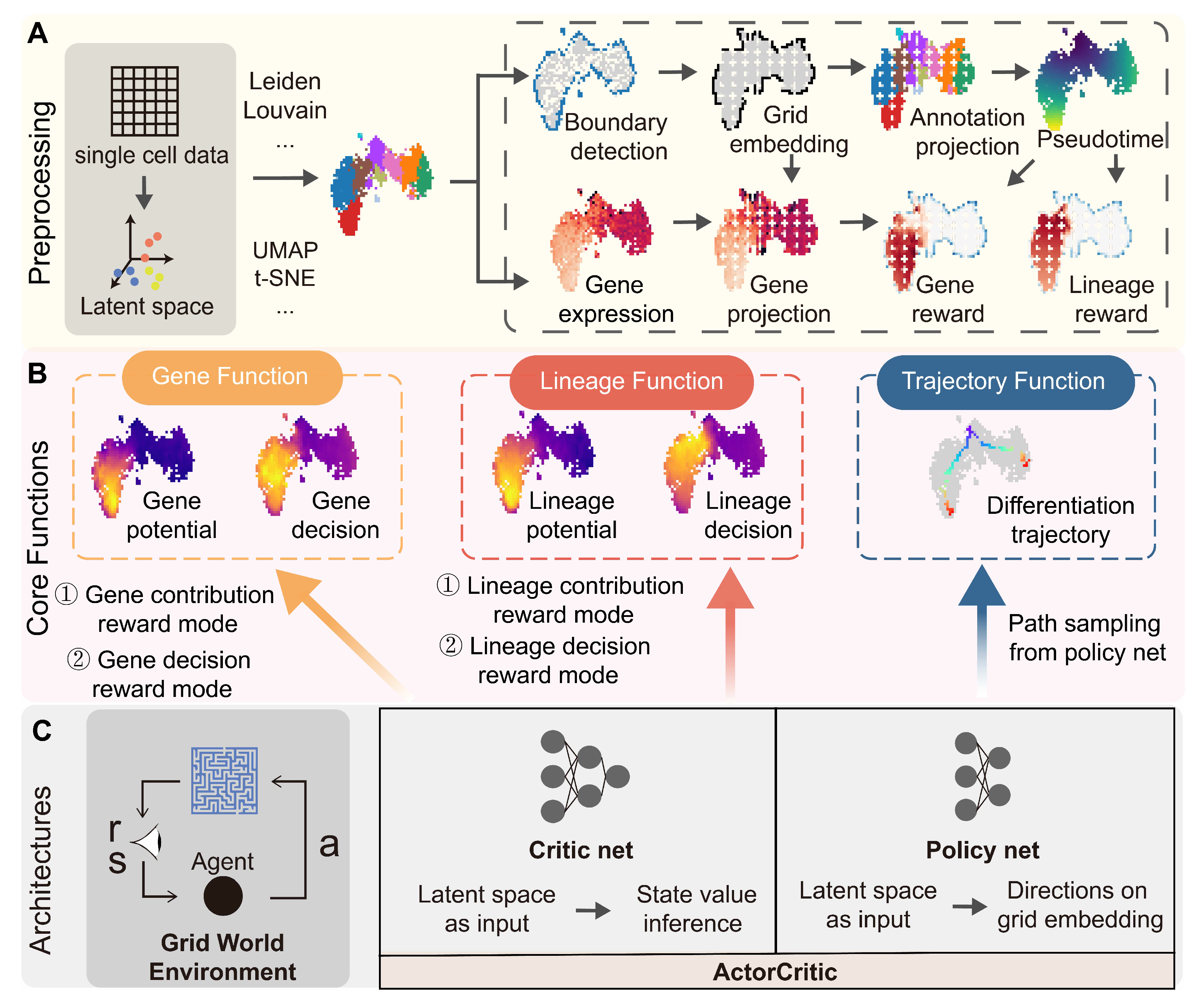
Appendix A
Figure A1.
Comprehensive analytical framework for scRL implementation and validation. (S-SUBS8, GSE132188) (A) Establishment of scRL efficacy through integration of tabular Q-learning validation on human hematopoietic cells and mouse endocrinogenesis datasets, with evaluation of pre-expression state identification using lineage-specific marker genes: GATA1 (erythroid), IRF8 (myeloid), EBF1 (lymphoid) for hematopoiesis, and Ngn3 (early), Fev (intermediate) for endocrinogenesis. (B) Cellular subpopulation-level analysis with cluster information projected onto grid space, establishing specific rewards for erythroid, myeloid and lymphoid lineages in hematopoietic dataset and early/late differentiation stages in endocrinogenesis dataset, with HSC (hematopoietic stem cell) and EP (endocrinogenesis progenitor) clusters as respective starting points. (C) Projection of derived final state values onto original embedding space for biological interpretation. (D) Training efficacy confirmation through convergence analysis of cumulative rewards from policy network and maximum state values from critic network over time.
![Biology 14 00679 g0a1]()
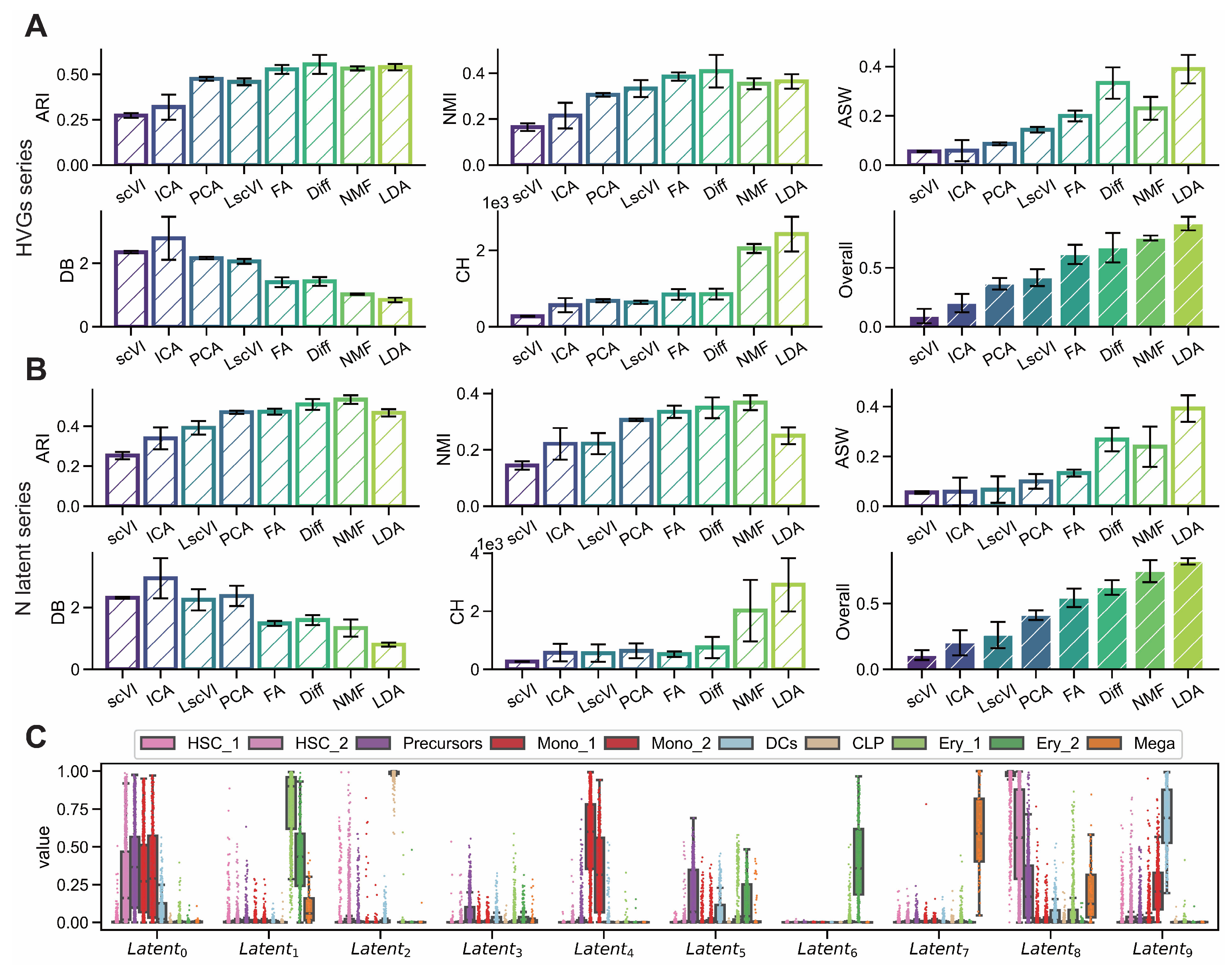
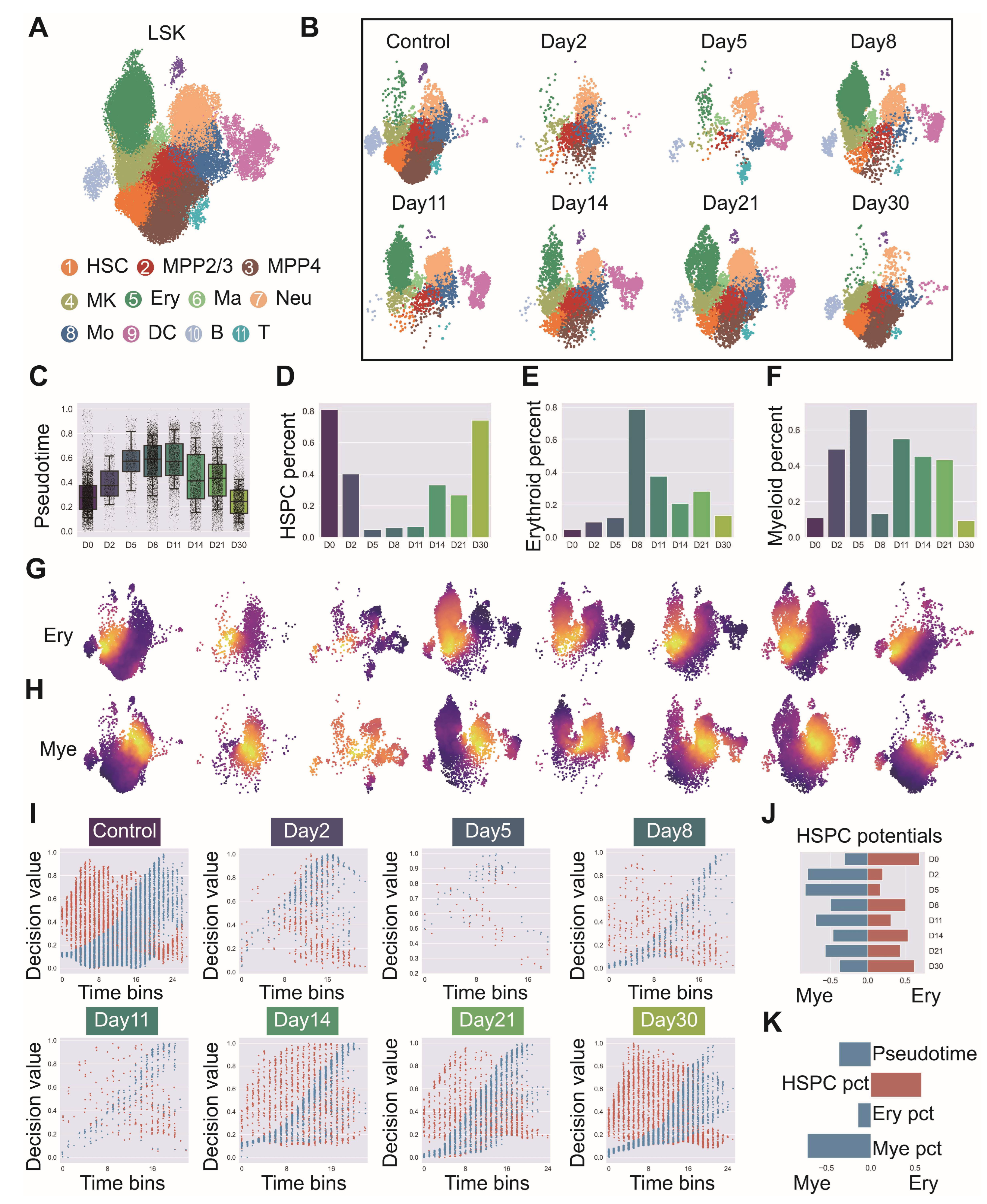
Figure A2.
LDA exhibits superior interpretability on endocrinogenesis dataset. (GSE132188) (A,B) Comparison of interpretability metrics including ARI, NMI, ASW, CH and DB for dimensionality reduction methods (scVI, ICA, PCA, LscVI, FA, Diff, NMF and LDA) evaluated across varying numbers of highly variable genes (1000, 2000, 3000, 4000, 5000) and latent space components (5, 10, 15, 20, 25). (C) Intensity distributions of latent components obtained by LDA across different subgroups.
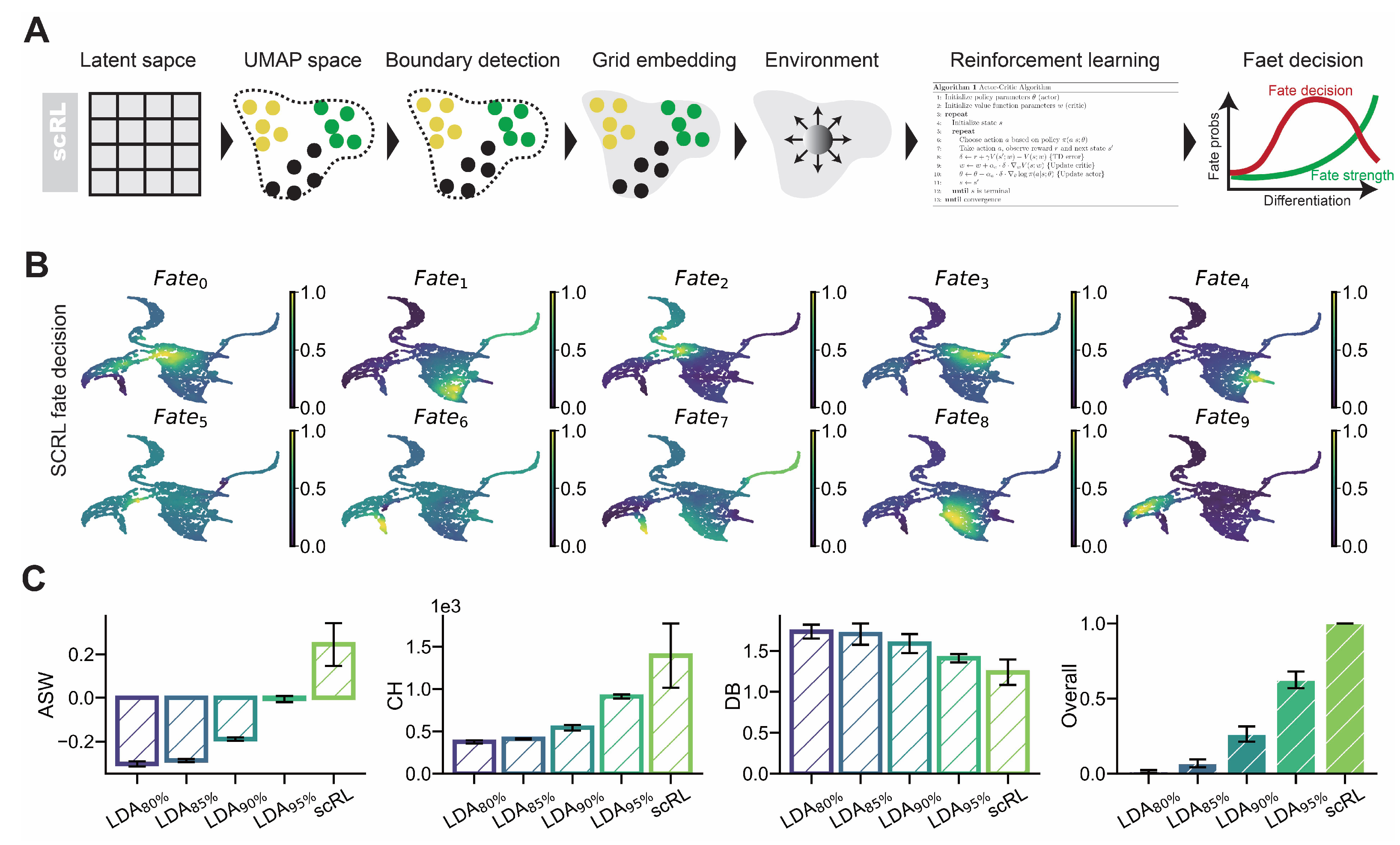
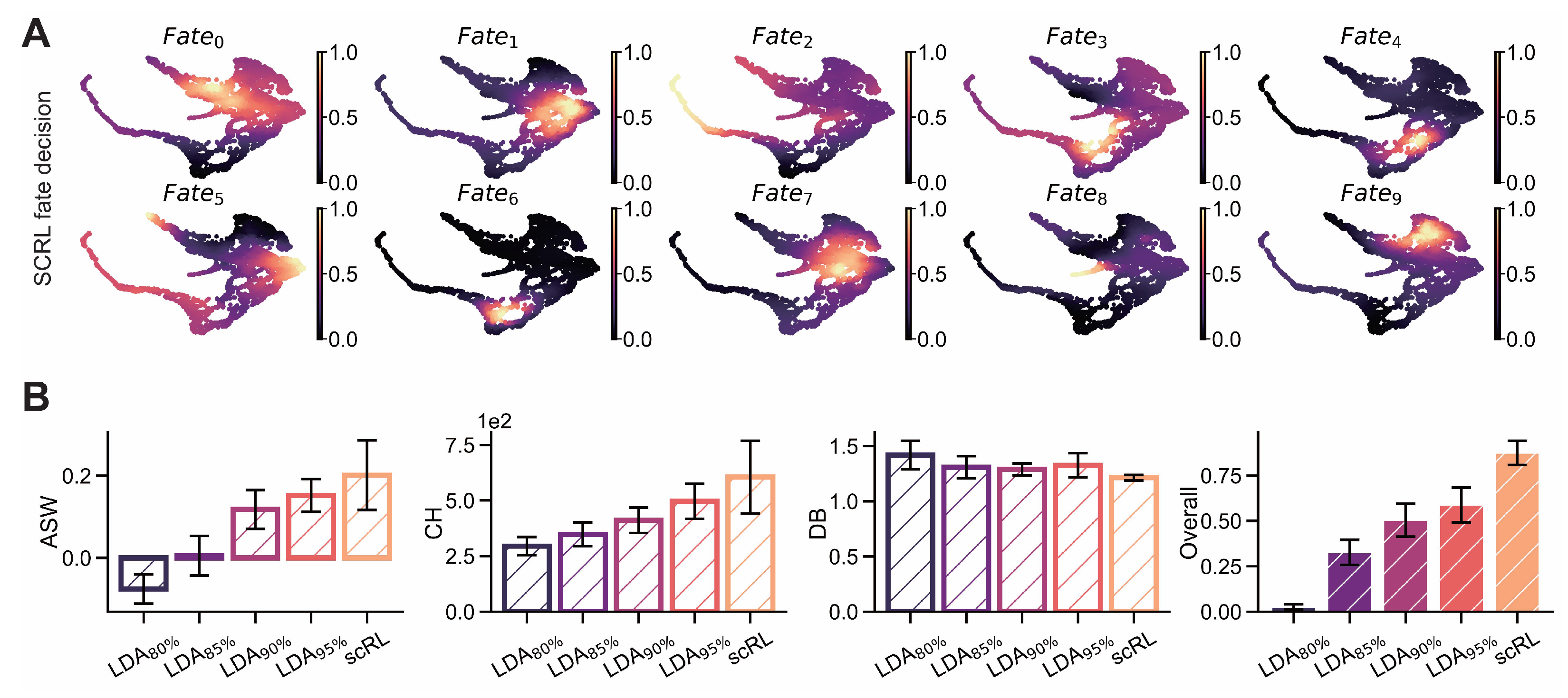
Figure A3.
scRL validation on endocrinogenesis dataset. (GSE132188) (A) Projection of fate decision intensity obtained by scRL onto UMAP embedding in endocrinogenesis dataset. (B) Comparison of scRL fate decision intensity with LDA percentile variants (95%, 90%, 85%, 80%) using ASW, CH and DB interpretability metrics.
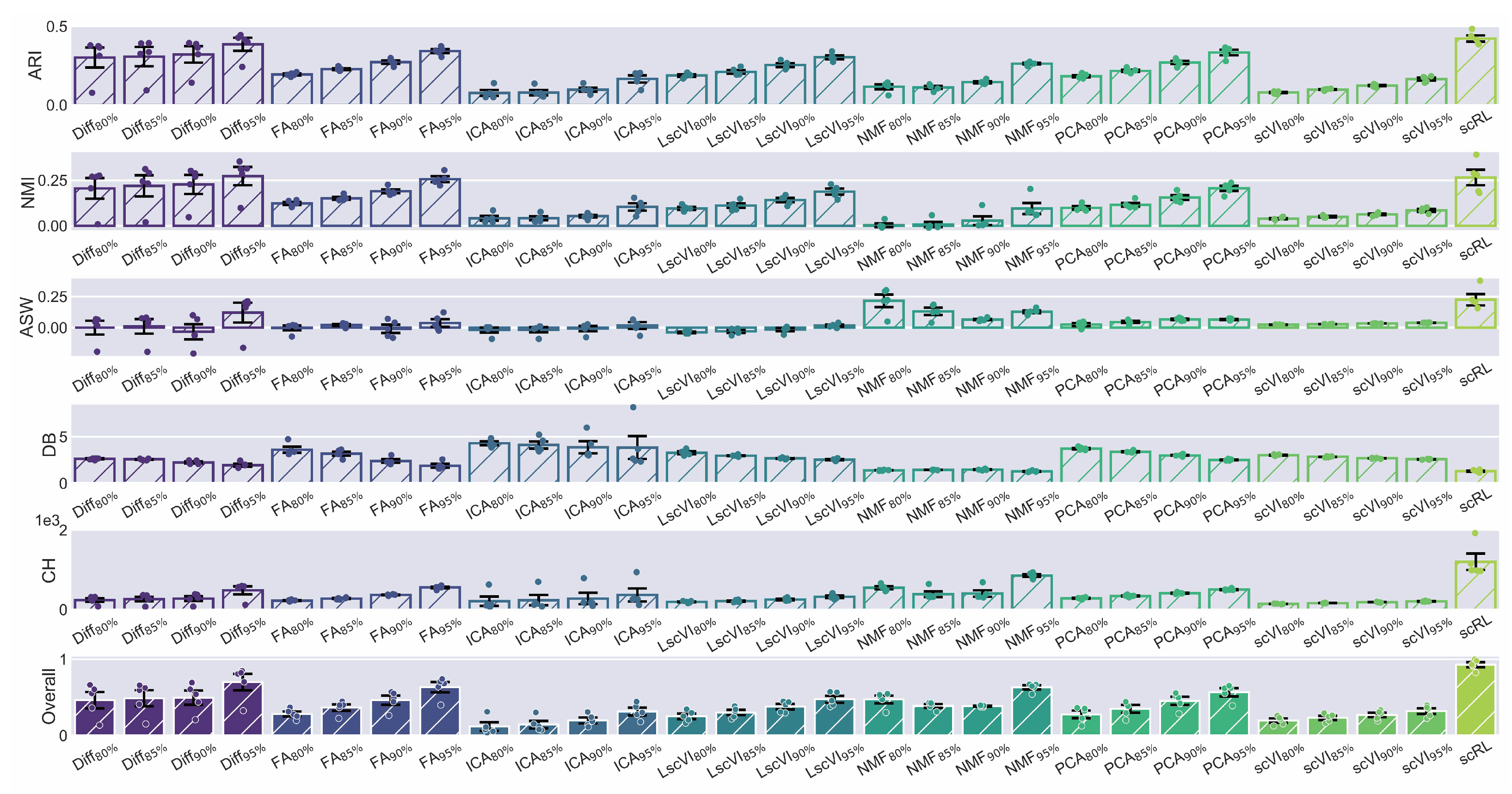
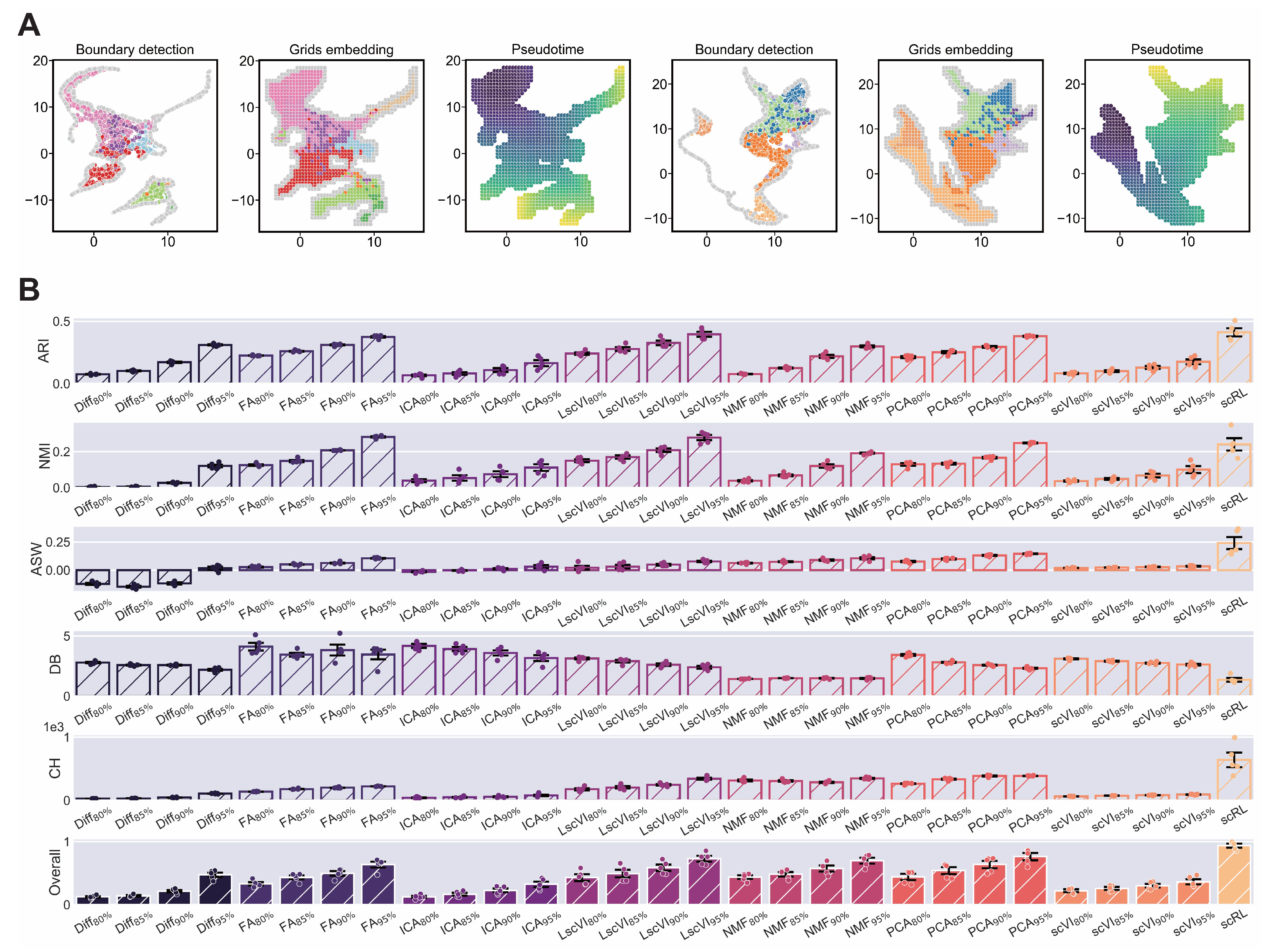
Figure A4.
scRL validation on endocrinogenesis dataset. (GSE132188) (A) Workflow of edge detection, grid embedding and pseudotime construction applied to hematopoietic and endocrinogenesis datasets. (B) Comprehensive comparison of interpretability metrics for scRL fate decision intensity against Diff, FA, ICA, LscVI, NMF, PCA and scVI at 95%, 90%, 85% and 80% percentile intensities on endocrinogenesis dataset.
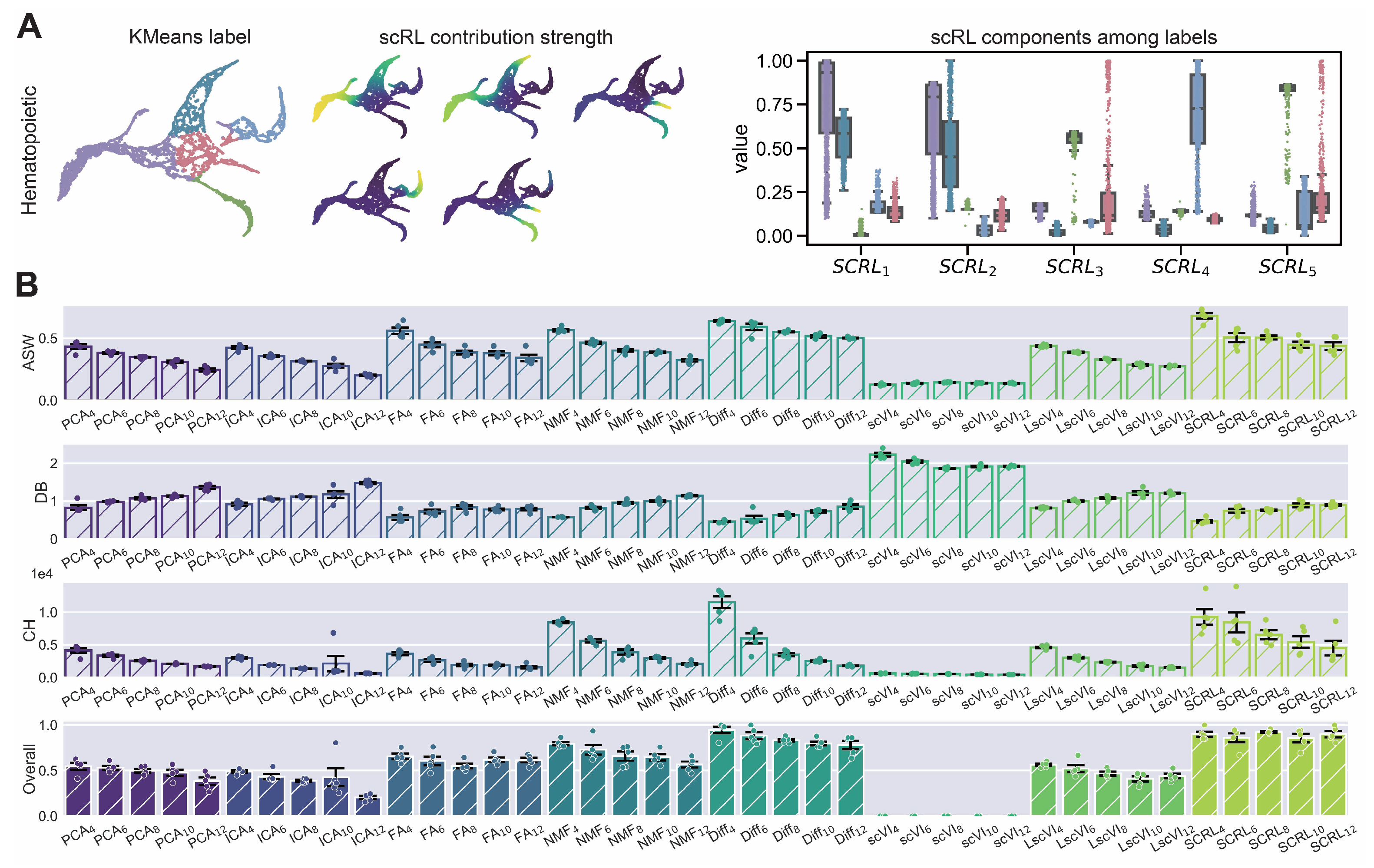
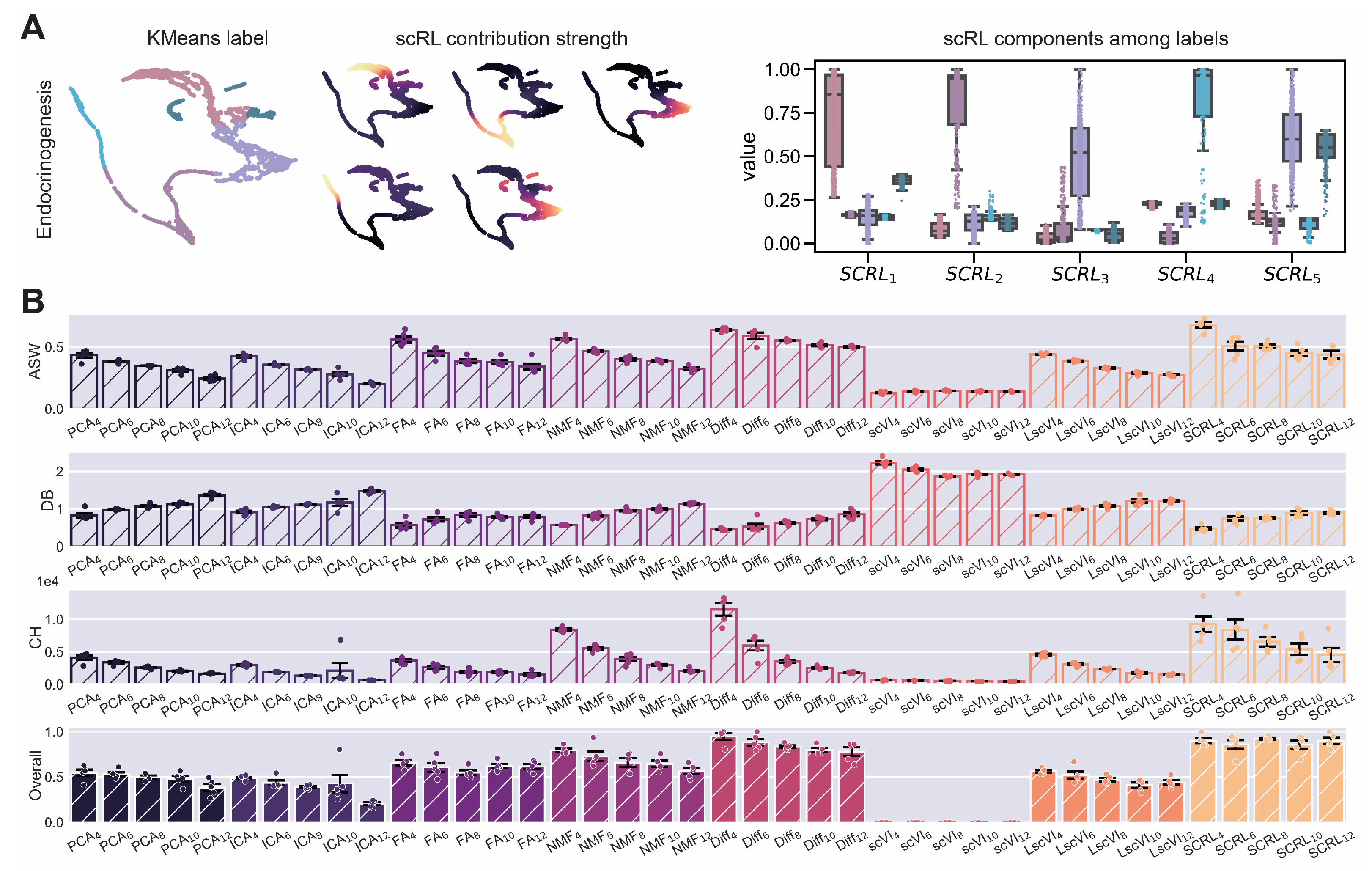
Figure A5.
scRL lineage intensity inference validation on endocrinogenesis dataset. (GSE132188) (A) Workflow demonstration showing KMeans clustering labels (left), scRL-derived contribution intensities (middle) and intensity distributions of each lineage branch across different labels (right). (B) Comprehensive comparison of scRL lineage contribution intensity against baseline methods (PCA, ICA, FA, NMF, Diff, scVI, LscVI) across KMeans cluster numbers (4, 6, 8, 10, 12) using ASW, DB and CH metrics, and overall composite scores.
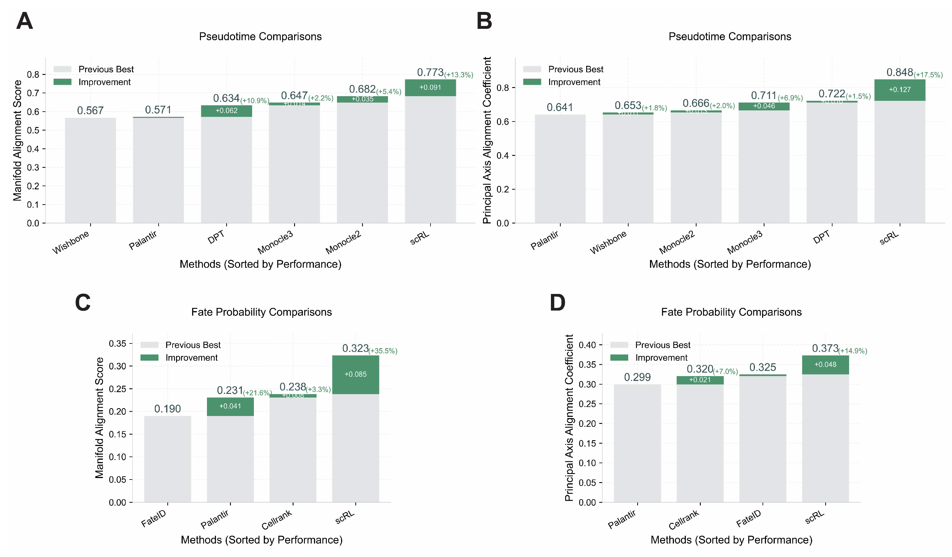
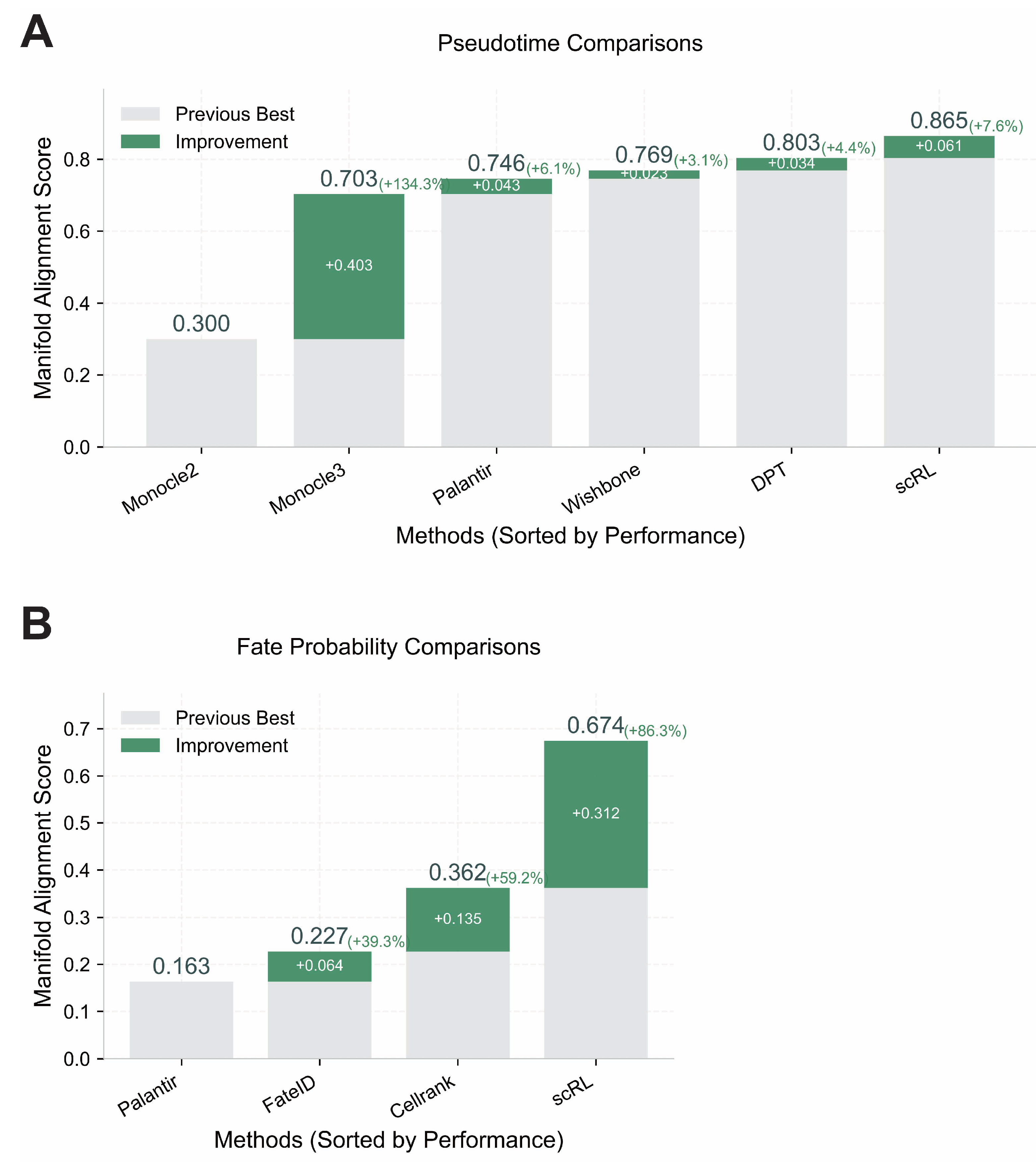
Figure A6.
Validation of scRL performance using Manifold Alignment Score metrics. (GSE132188, GSE117498) (A) Pseudotime reconstruction comparison between scRL and baseline methods (Monocle2, Monocle3, Palantir, Wishbone, DPT) on endocrinogenesis dataset showing scRL’s superior performance with +0.061 improvement over previous best method. (B) Fate probability inference comparison between scRL and established methods (Palantir, FateID, CellRank) on phenotypical HSC dataset demonstrating scRL’s substantial +0.312 improvement over previous best method.
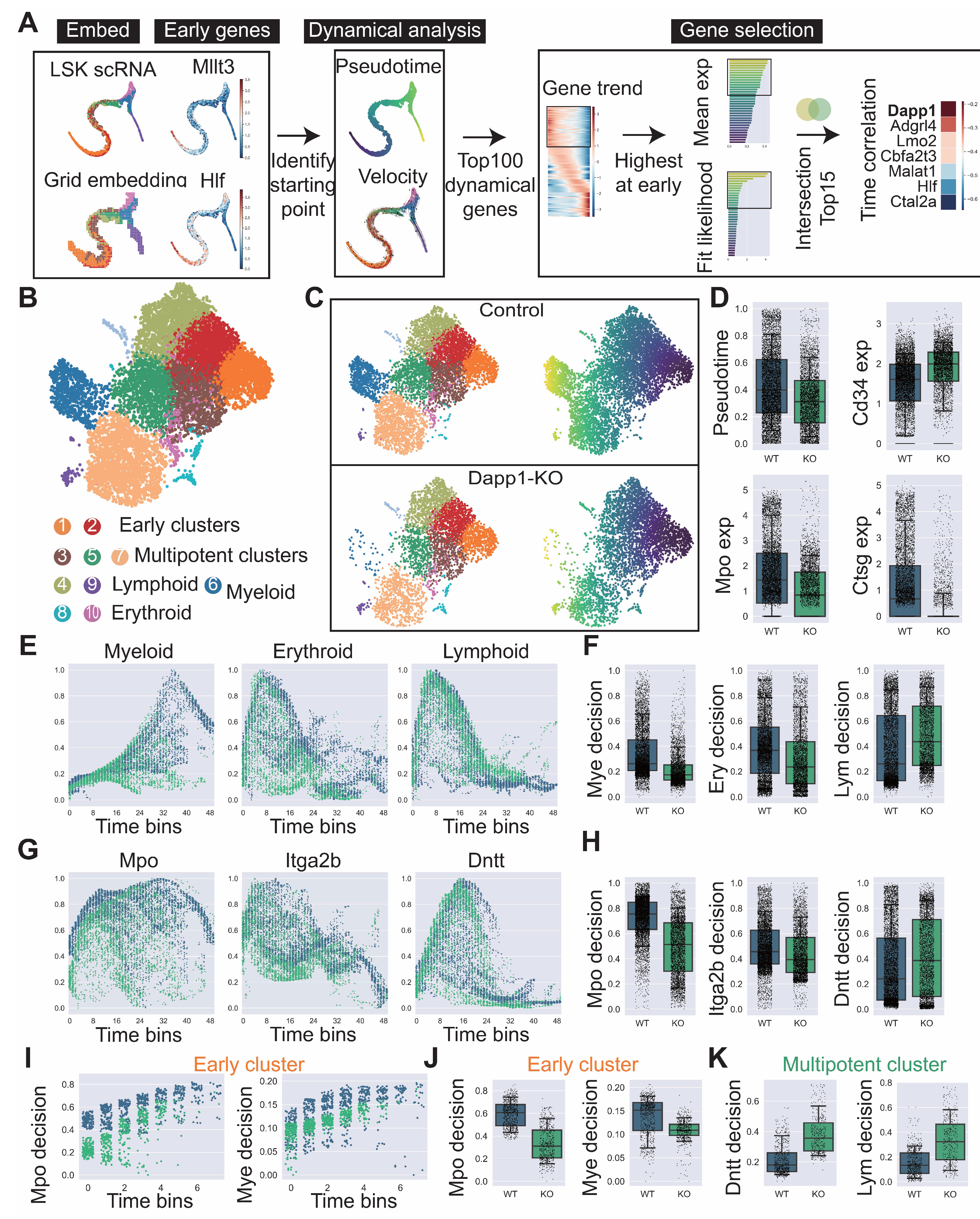
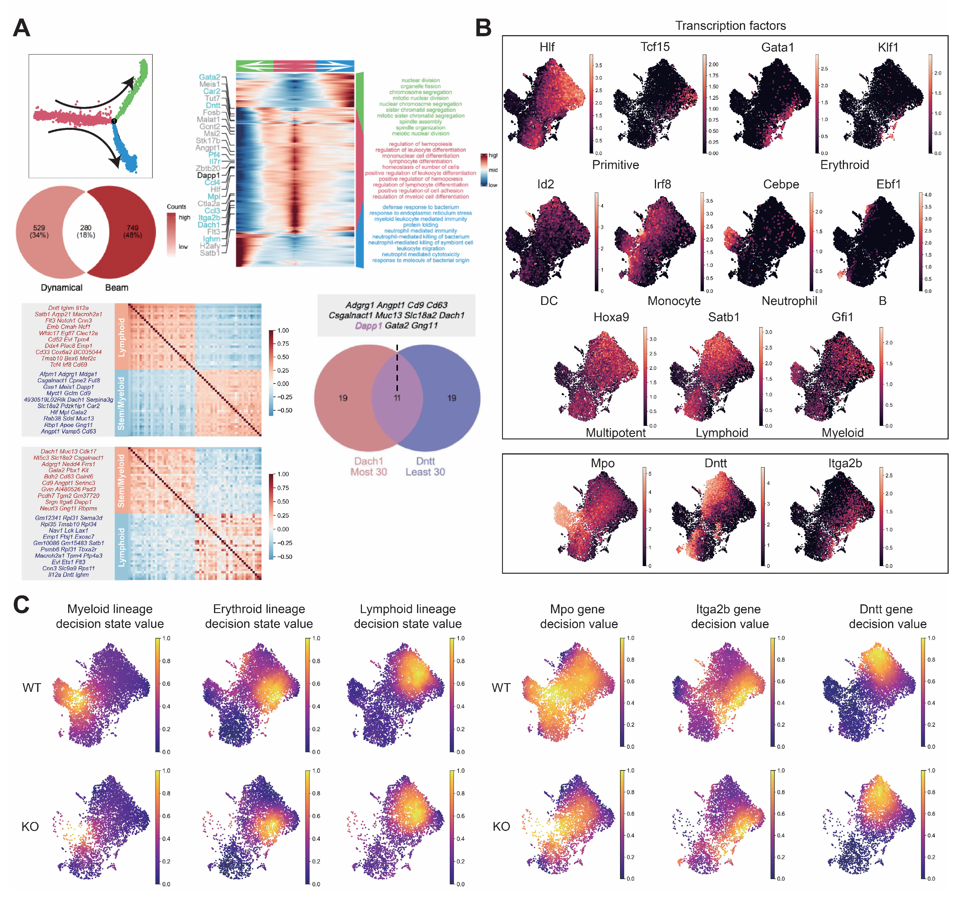
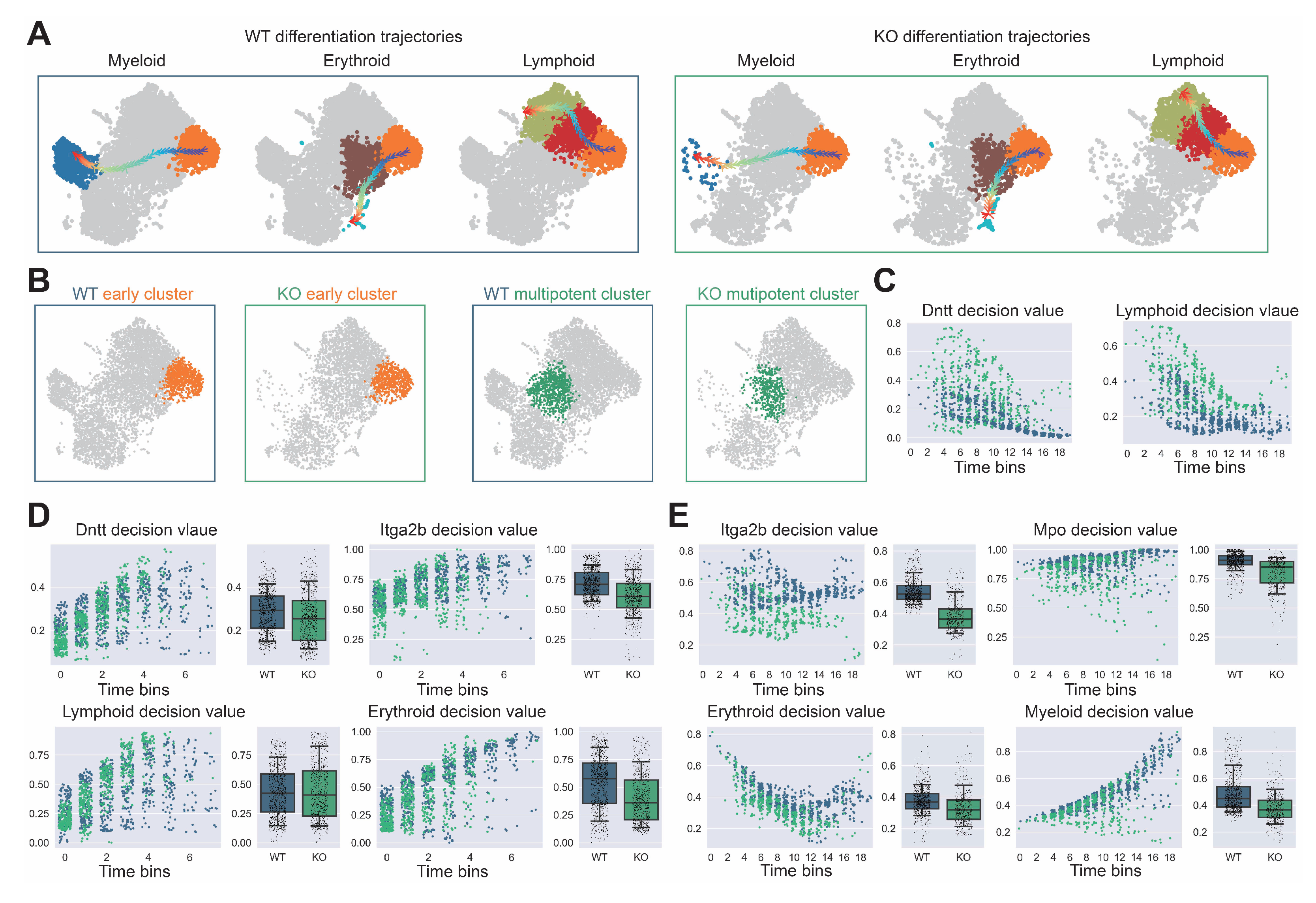
Figure A7.
Comprehensive analysis of hematopoietic differentiation regulators and validation of Dapp1’s role in lineage contribution. (GSE277292) (A) Monocle2 differentiation trajectory analysis showing intersection of dynamical genes and BEAM (Branching Expression Analysis Modeling) test significant genes yielding 280 genes with Dapp1 as an early gene. Gene expression trends across trajectories with GOBP enrichment analysis. Gene correlation analysis of LSK single-cell data from GSE136341 and GSE145491 showing Dach1 and Dntt correlation patterns with associated gene sets and intersection analysis. (B) Transcription factor expression patterns critical for hematopoietic lineage identification on UMAP, including Hlf and Tcf15 for primitive HSCs, Gata1 and Klf1 for erythroid bias, Id2 for dendritic cells, Irf8 for monocytes, Cebpe for neutrophils, Ebf1 for B cells, Hoxa9 for multipotency, Satb1 for lymphoid bias and Gfi1 for myeloid bias. Expression patterns of lineage markers Mpo, Dntt and Itga2b are also displayed. (C) Comparative analysis of lineage decision intensities for myeloid, erythroid and lymphoid lineages, along with gene decision intensities for Mpo, Itga2b and Dntt between Dapp1 knockout and control groups.
![Biology 14 00679 g0a7]()
Figure A8.
Detailed trajectory analysis of lineage decision dynamics following Dapp1 knockout in hematopoietic differentiation. (GSE277292) (A) Myeloid, erythroid and lymphoid differentiation trajectories comparing wild-type (left) and knockout (right) conditions. (B) Early (left) and multipotent (right) cluster identification within UMAP embedding for wild-type and knockout conditions. (C) Dntt gene decision value and lymphoid lineage decision value progression along pseudotime within early cluster populations. (D) Left panel: Dntt gene decision value and lymphoid lineage decision value along pseudotime within multipotent cluster. Right panel: Itga2b gene decision value and erythroid lineage decision value along pseudotime within early cluster. (E) Left panel: Itga2b gene decision value and erythroid lineage decision value along pseudotime within multipotent cluster. Right panel: Mpo gene decision value and myeloid lineage decision value along pseudotime within multipotent cluster.
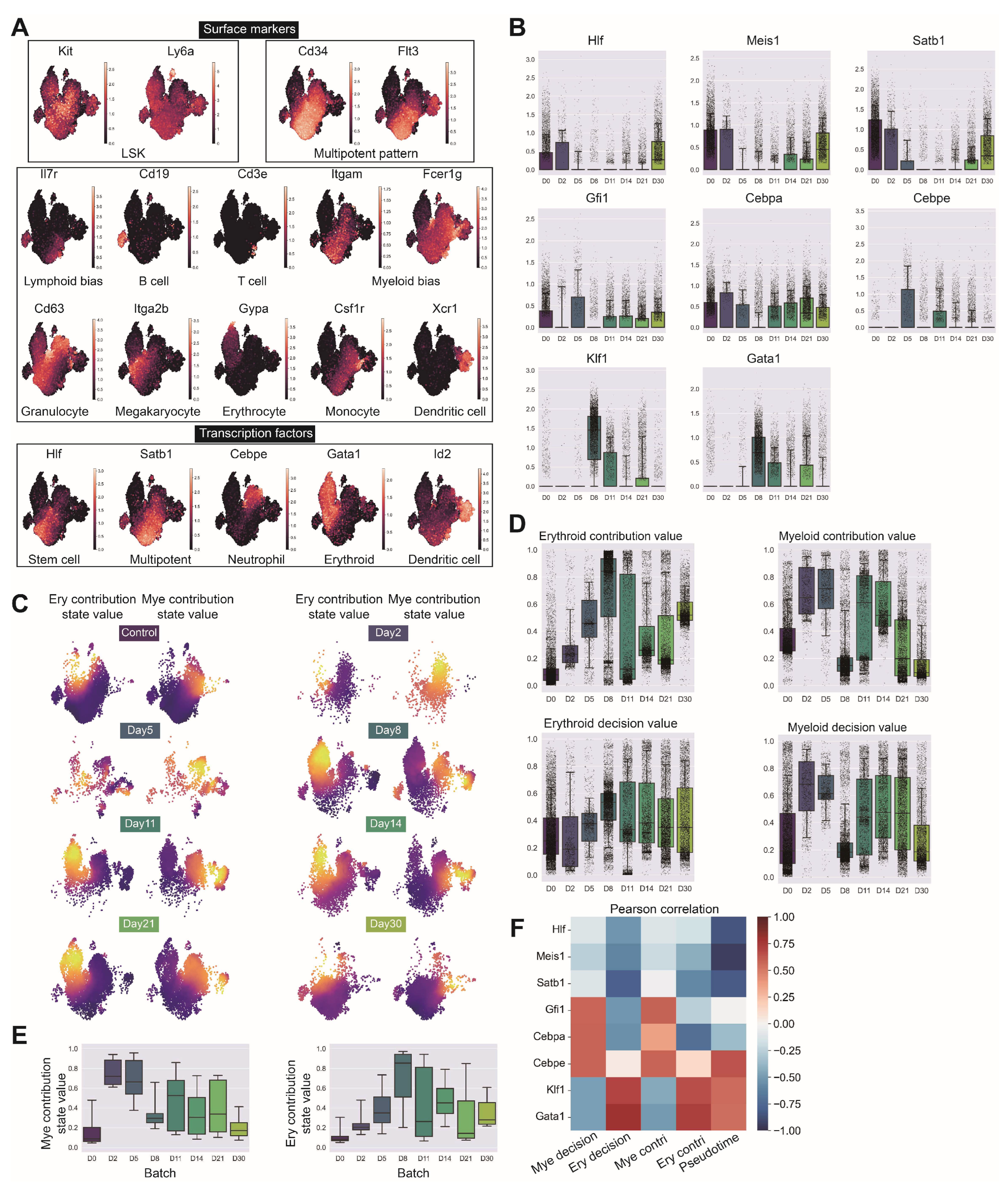
Figure A9.
Comprehensive validation of LSK cell identification and lineage contribution dynamics following irradiation. (GSE278673) (A) Expression patterns of Kit (c-Kit) and Ly6a (Sca-1) genes validating LSK cell identification, Cd34 and Flt3 indicating multipotent progenitor components, key surface markers for hematopoietic lineage identification including Il7r (lymphoid bias), Cd19 (B cells), Cd3e (T cells), Itgam and Fcer1g (myeloid bias), Cd63 (granulocyte bias), Itga2b (megakaryocytic bias), Gypa (Erythrocytes), Csf1r (monocytes) and Xcr1 (dendritic cells), and critical transcription factors Hlf (stem cells), Satb1 (multipotent progenitors), Cebpe (neutrophil lineage), Gata1 (erythroid lineage) and Id2 (dendritic cell lineage). (B) Temporal expression patterns of primitive factors (Hlf, Meis1, Satb1, Hoxa9), myeloid factors (Spi1, Gfi1, Cebpa, Cebpe) and erythroid factors (Klf1, Gata1) across irradiation recovery time course. (C) Erythroid and myeloid contribution values at different time points projected on UMAP embedding with corresponding box plot quantification. (D,E) Comparative analysis of erythroid and myeloid lineage contribution and decision intensities between normal LSK and irradiated samples across all time points. (F) Correlation heatmap of lineage decision values at each time point against expression of primitive genes (Hlf, Meis1, Satb1), myeloid genes (Gfi1, Cebpa, Cebpe) and erythroid genes (Klf1, Gata1).
![Biology 14 00679 g0a9]()
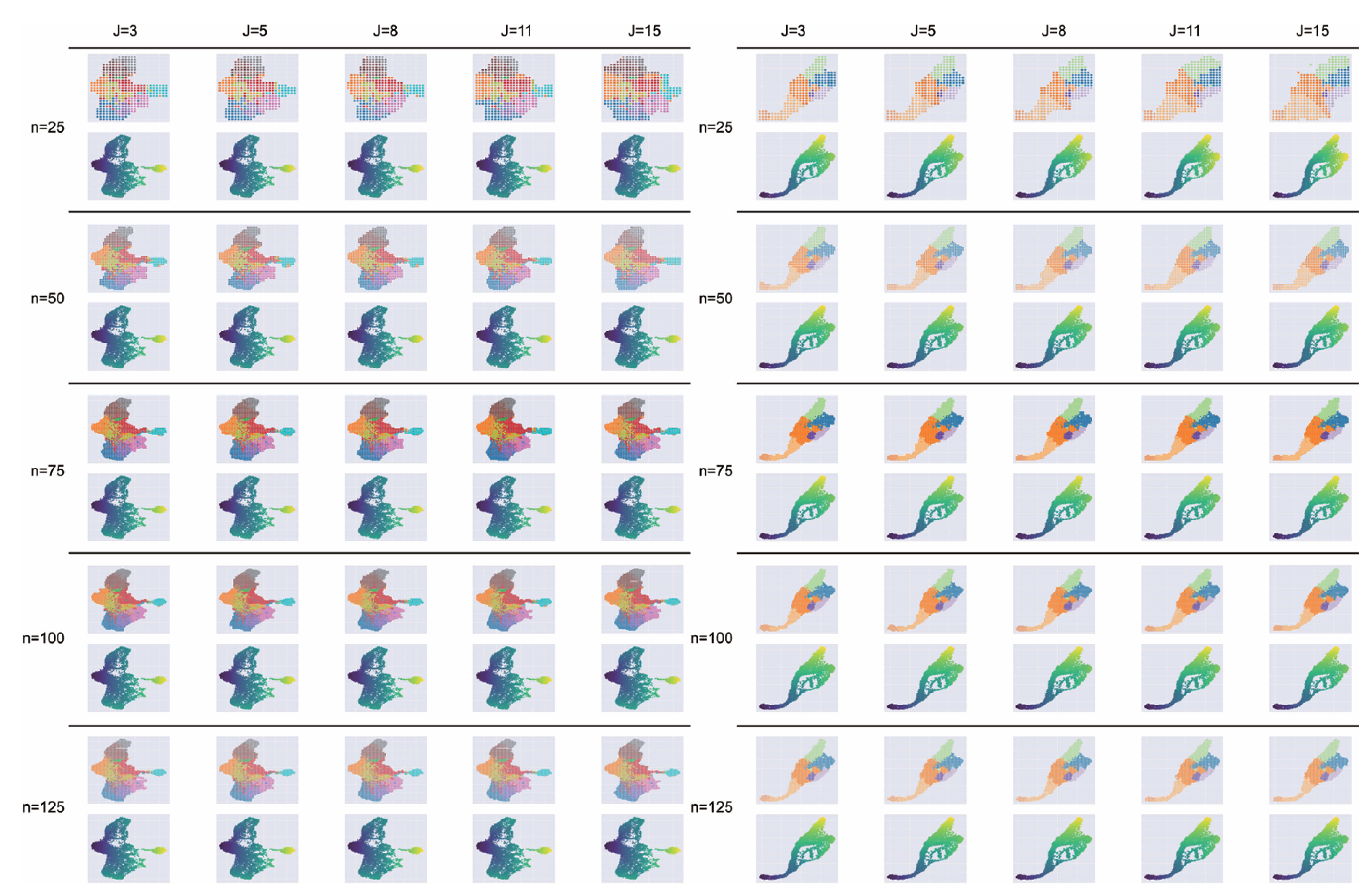
Figure A10.
Impact of hyperparameters n and j on grid embedding. Performance was evaluated on the hematopoiesis (left) and endocrinogenesis (right) datasets using grid size , 50, 75, 100, 125 and neighborhood parameter , 5, 8, 11, 15.
Figure A10.
Impact of hyperparameters n and j on grid embedding. Performance was evaluated on the hematopoiesis (left) and endocrinogenesis (right) datasets using grid size , 50, 75, 100, 125 and neighborhood parameter , 5, 8, 11, 15.
Table A1.
LDA performance improvements over baseline methods on endocrinogenesis dataset across HVG sizes.
Table A1.
LDA performance improvements over baseline methods on endocrinogenesis dataset across HVG sizes.
| Method | NMI | ARI | ASW | DB | CH | Overall |
|---|
| LDA vs. scVI | +0.258 | +0.187 | +0.379 | +1.613 | +1416.596 | +0.806 |
| LDA vs. ICA | +0.251 | +0.157 | +0.349 | +1.869 | +1411.359 | +0.789 |
| LDA vs. LscVI | +0.061 | −0.006 | +0.306 | +1.254 | +1061.209 | +0.455 |
| LDA vs. Diff | +0.012 | +0.022 | +0.165 | +0.832 | +1166.559 | +0.347 |
| LDA vs. PCA | +0.012 | −0.060 | +0.254 | +0.971 | +1022.558 | +0.341 |
| LDA vs. FA | −0.023 | −0.100 | +0.159 | +0.145 | +1085.451 | +0.173 |
| LDA vs. NMF | −0.074 | −0.084 | +0.117 | +0.147 | +744.455 | +0.087 |
Table A2.
LDA performance improvements over baseline methods on endocrinogenesis dataset across latent space sizes.
Table A2.
LDA performance improvements over baseline methods on endocrinogenesis dataset across latent space sizes.
| Method | NMI | ARI | ASW | DB | CH | Overall |
|---|
| LDA vs. scVI | +0.278 | +0.186 | +0.370 | +1.579 | +1506.128 | +0.839 |
| LDA vs. ICA | +0.189 | +0.124 | +0.337 | +1.799 | +1495.191 | +0.765 |
| LDA vs. LscVI | +0.099 | +0.057 | +0.329 | +1.514 | +1109.556 | +0.605 |
| LDA vs. Diff | +0.034 | +0.028 | +0.206 | +0.906 | +1323.790 | +0.420 |
| LDA vs. PCA | +0.027 | -0.082 | +0.266 | +1.486 | +1218.136 | +0.410 |
| LDA vs. FA | +0.023 | -0.060 | +0.200 | +0.503 | +1270.592 | +0.313 |
| LDA vs. NMF | +0.004 | -0.054 | +0.185 | +0.428 | +719.630 | +0.236 |
Table A3.
scRL performance improvements over LDA percentile variants on endocrinogenesis dataset.
Table A3.
scRL performance improvements over LDA percentile variants on endocrinogenesis dataset.
| Method | ARI | NMI | ASW | CH | DB | Overall |
|---|
| scRL vs. | +0.219 | +0.122 | +0.277 | +310.840 | +0.205 | +0.848 |
| scRL vs. | +0.176 | +0.104 | +0.196 | +256.830 | +0.095 | +0.549 |
| scRL vs. | +0.099 | +0.055 | +0.083 | +194.023 | +0.076 | +0.371 |
| scRL vs. | +0.025 | −0.012 | +0.049 | +108.108 | +0.112 | +0.287 |
Table A4.
scRL fate decision performance improvements over baseline methods on endocrinogenesis dataset.
Table A4.
scRL fate decision performance improvements over baseline methods on endocrinogenesis dataset.
| Method | NMI | ARI | ASW | DB | CH | Overall |
|---|
| scRL vs. | +0.337 | +0.236 | +0.364 | +1.436 | +615.913 | +0.811 |
| scRL vs. | +0.310 | +0.234 | +0.389 | +1.218 | +610.215 | +0.793 |
| scRL vs. | +0.240 | +0.213 | +0.359 | +1.222 | +596.458 | +0.722 |
| scRL vs. | +0.102 | +0.120 | +0.224 | +0.831 | +534.217 | +0.461 |
| scRL vs. | +0.187 | +0.115 | +0.213 | +2.754 | +503.551 | +0.605 |
| scRL vs. | +0.152 | +0.092 | +0.190 | +2.089 | +461.722 | +0.502 |
| scRL vs. | +0.100 | +0.033 | +0.177 | +2.471 | +440.212 | +0.439 |
| scRL vs. | +0.037 | −0.041 | +0.134 | +2.100 | +418.401 | +0.300 |
| scRL vs. | +0.345 | +0.201 | +0.255 | +2.819 | +599.145 | +0.812 |
| scRL vs. | +0.331 | +0.186 | +0.244 | +2.557 | +592.465 | +0.770 |
| scRL vs. | +0.303 | +0.165 | +0.229 | +2.227 | +584.174 | +0.709 |
| scRL vs. | +0.248 | +0.129 | +0.210 | +1.804 | +563.078 | +0.612 |
| scRL vs. | +0.171 | +0.090 | +0.219 | +1.772 | +465.352 | +0.506 |
| scRL vs. | +0.134 | +0.070 | +0.210 | +1.450 | +435.556 | +0.443 |
| scRL vs. | +0.085 | +0.032 | +0.192 | +1.251 | +393.053 | +0.351 |
| scRL vs. | +0.016 | −0.037 | +0.164 | +1.037 | +297.412 | +0.207 |
| scRL vs. | +0.335 | +0.202 | +0.178 | +0.066 | +325.897 | +0.499 |
| scRL vs. | +0.287 | +0.171 | +0.167 | +0.134 | +332.902 | +0.452 |
| scRL vs. | +0.193 | +0.120 | +0.151 | +0.123 | +353.477 | +0.362 |
| scRL vs. | +0.113 | +0.049 | +0.134 | +0.116 | +291.898 | +0.238 |
| scRL vs. | +0.200 | +0.111 | +0.164 | +2.066 | +376.044 | +0.495 |
| scRL vs. | +0.160 | +0.107 | +0.142 | +1.450 | +304.960 | +0.395 |
| scRL vs. | +0.117 | +0.074 | +0.110 | +1.214 | +253.100 | +0.298 |
| scRL vs. | +0.032 | −0.007 | +0.095 | +0.961 | +252.420 | +0.173 |
| scRL vs. | +0.330 | +0.203 | +0.221 | +1.741 | +577.491 | +0.713 |
| scRL vs. | +0.312 | +0.191 | +0.217 | +1.546 | +568.437 | +0.678 |
| scRL vs. | +0.283 | +0.173 | +0.213 | +1.392 | +559.935 | +0.634 |
| scRL vs. | +0.237 | +0.140 | +0.206 | +1.267 | +548.500 | +0.571 |
Table A5.
scRL lineage contribution performance improvements over baseline methods across different cluster numbers on endocrinogenesis dataset.
Table A5.
scRL lineage contribution performance improvements over baseline methods across different cluster numbers on endocrinogenesis dataset.
| Method | ASW | DB | CH | Overall |
|---|
| scRL vs. | +0.247 | +0.359 | +5121.830 | +0.353 |
| scRL vs. | +0.124 | +0.235 | +5058.890 | +0.329 |
| scRL vs. | +0.157 | +0.310 | +3963.771 | +0.426 |
| scRL vs. | +0.137 | +0.237 | +3330.795 | +0.379 |
| scRL vs. | +0.194 | +0.465 | +2821.714 | +0.515 |
| scRL vs. | +0.256 | +0.447 | +6269.940 | +0.409 |
| scRL vs. | +0.150 | +0.312 | +6535.205 | +0.425 |
| scRL vs. | +0.189 | +0.353 | +5198.874 | +0.535 |
| scRL vs. | +0.169 | +0.280 | +3284.407 | +0.430 |
| scRL vs. | +0.235 | +0.578 | +3874.281 | +0.694 |
| scRL vs. | +0.119 | +0.100 | +5613.054 | +0.242 |
| scRL vs. | +0.058 | +0.023 | +5792.529 | +0.254 |
| scRL vs. | +0.120 | +0.080 | +4634.559 | +0.375 |
| scRL vs. | +0.069 | +0.112 | +3547.165 | +0.236 |
| scRL vs. | +0.096 | +0.106 | +2951.559 | +0.284 |
| scRL vs. | +0.114 | +0.105 | +816.813 | +0.105 |
| scRL vs. | +0.042 | +0.077 | +2848.851 | +0.131 |
| scRL vs. | +0.103 | +0.196 | +2651.048 | +0.265 |
| scRL vs. | +0.061 | +0.103 | +2414.816 | +0.210 |
| scRL vs. | +0.114 | +0.240 | +2419.564 | +0.334 |
| scRL vs. | +0.041 | +0.012 | −2261.901 | −0.048 |
| scRL vs. | −0.086 | +0.212 | +2454.264 | −0.024 |
| scRL vs. | −0.047 | +0.133 | +3041.397 | +0.091 |
| scRL vs. | −0.069 | +0.161 | +2894.393 | +0.059 |
| scRL vs. | −0.064 | +0.043 | +2708.683 | +0.120 |
| scRL vs. | +0.551 | +1.761 | +8639.039 | +0.899 |
| scRL vs. | +0.368 | +1.301 | +7855.647 | +0.859 |
| scRL vs. | +0.360 | +1.106 | +5999.717 | +0.924 |
| scRL vs. | +0.308 | +1.024 | +4944.921 | +0.856 |
| scRL vs. | +0.300 | +1.019 | +4055.950 | +0.899 |
| scRL vs. | +0.241 | +0.350 | +4669.743 | +0.336 |
| scRL vs. | +0.119 | +0.255 | +5366.970 | +0.337 |
| scRL vs. | +0.177 | +0.320 | +4190.457 | +0.456 |
| scRL vs. | +0.161 | +0.321 | +3663.236 | +0.447 |
| scRL vs. | +0.164 | +0.311 | +2998.675 | +0.461 |


