
COVID-19 in Italy: Is the Mortality Analysis a Way to Estimate How the Epidemic Lasts?


Abstract
:Simple Summary
Abstract
1. Introduction
2. Materials and Methods
2.1. Data
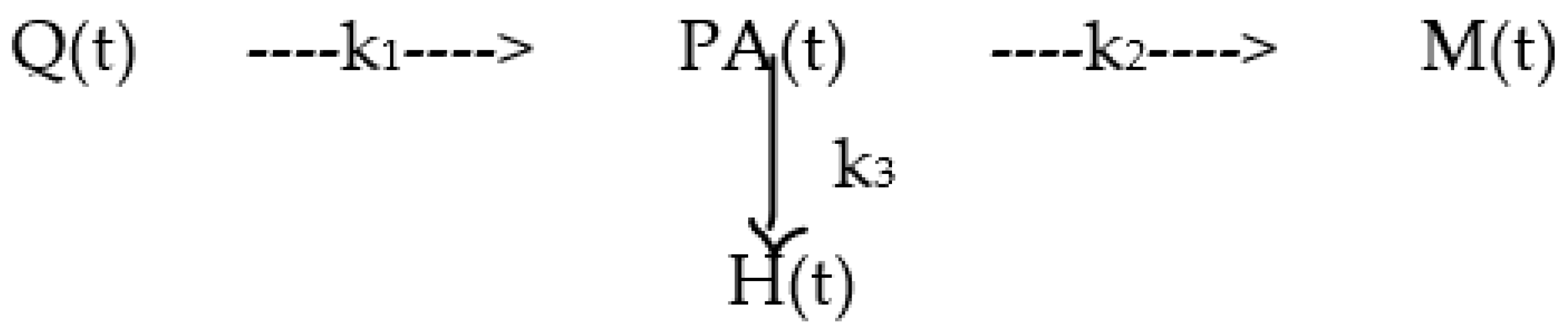
2.2. Model
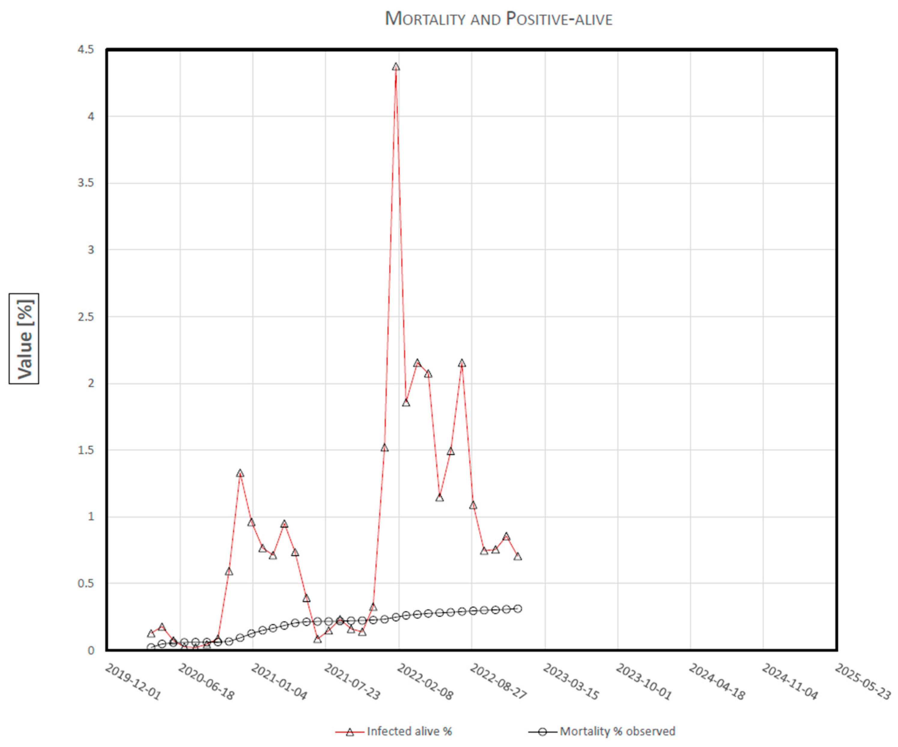
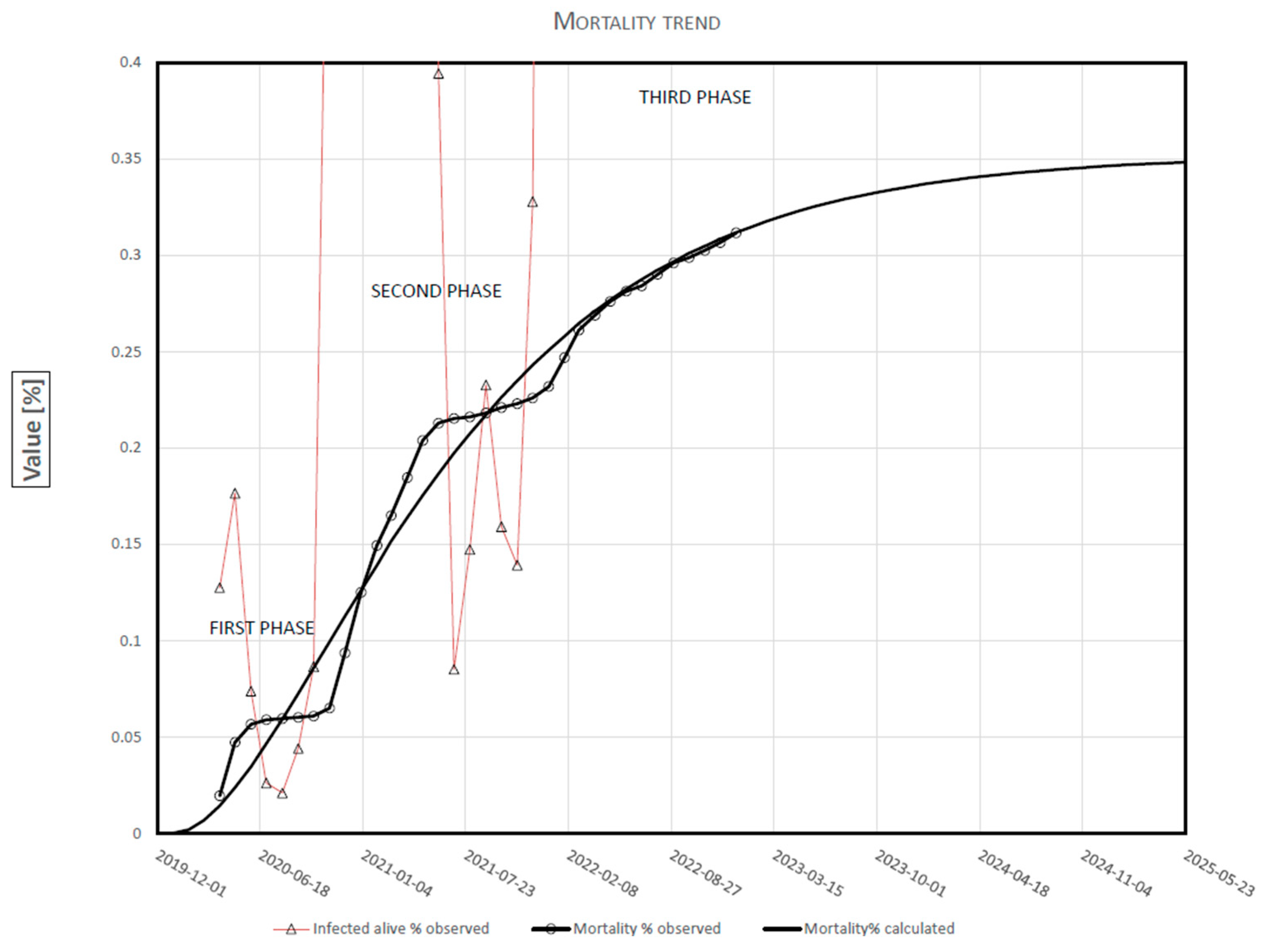
- The trend of mortality (observed data) develops in phases;
- The trend of positive-alive (observed data) shows some peaks from mid-2021;
- Since the overall outcome of an epidemic depends on the number of deaths, mortality analysis could lead to predicting its duration.
3. Results
4. Discussion
5. Conclusions
Author Contributions
Funding
Institutional Review Board Statement
Informed Consent Statement
Data Availability Statement
Conflicts of Interest
References
- WHO. WHO Coronavirus (COVID-19) Dashboard. Available online: https://covid19.who.int/ (accessed on 25 March 2023).
- Nistal, R.; de la Sen, M.; Gabirondo, J.; Alonso-Quesada, S.; Garrido, A.J.; Garrido, I. A Modelization of the propagation of COVID-19 in regions of Spain and Italy with evaluation of the transmission rates related to the intervention measures. Biology 2021, 10, 121. [Google Scholar] [CrossRef] [PubMed]
- Ferrari, L.; Gerardi, G.; Manzi, G.; Micheletti, A.; Nicolussi, F.; Biganzoli, E.; Salini, S. Modeling provincial COVID-19 epidemic data using an Adjusted Time-Dependent SIRD Model. Int. J. Environ. Res. Public Health 2021, 18, 6563. [Google Scholar] [CrossRef] [PubMed]
- Mahikul, W.; Chotsiri, P.; Ploddi, K.; Panngum, W. Evaluating the Impact of intervention strategies on the first wave and predicting the second wave of COVID-19 in Thailand: A mathematical modeling study. Biology 2021, 10, 80. [Google Scholar] [CrossRef] [PubMed]
- Fonseca i Casas, P.; García i Carrasco, V.; Garcia i Subirana, J. SEIRD COVID-19 formal characterization and model comparison validation. Appl. Sci. 2020, 10, 5162. [Google Scholar] [CrossRef]
- Liu, X.-X.; Yang, J.; Fong, S.; Dey, N.; Millham, R.C.; Fiaidhi, J. All-people-test-based methods for COVID-19 infectious disease dynamics simulation model: Towards citywide COVID testing. Int. J. Environ. Res. Public Health 2022, 19, 10959. [Google Scholar] [CrossRef] [PubMed]
- Demongeot, J.; Magal, P. Spectral method in epidemic time series: Application to COVID-19 pandemic. Biology 2022, 11, 1825. [Google Scholar] [CrossRef] [PubMed]
- Perone, G. Using the SARIMA model to forecast the fourth global wave of cumulative deaths from COVID-19: Evidence from 12 hard-hit big countries. Econometrics 2022, 10, 18. [Google Scholar] [CrossRef]
- Wang, Y.; Xu, C.; Yao, S.; Wang, L.; Zhao, Y.; Ren, J.; Li, Y. Estimating the COVID-19 prevalence and mortality using a novel data-driven hybrid model based on ensemble empirical mode decomposition. Sci. Rep. 2021, 11, 1–17. [Google Scholar] [CrossRef] [PubMed]
- Friedman, J.; Liu, P.; Troeger, C.E.; Carter, A.; Reiner, R.C., Jr.; Ryan, M.B.; Collins, J.; Lim, S.S.; Pigott, D.M.; Vos, T.; et al. Predictive performance of international COVID-19 mortality forecasting model. Nat. Commun. 2021, 12, 2609. [Google Scholar] [CrossRef] [PubMed]
- MIT Operations Research Center. MIT DELPHI Epidemiological Case Predictions COVID. Analytics. Available online: https://github.com/COVIDAnalytics/website/tree/master (accessed on 25 March 2023).
- Los Alamos National Laboratory COVID-19 Team. Los Alamos Natinoal Laboratory COVID-19 Confirmed and Forecasted Case Data. Available online: https://covid-19.bsvgateway.org/ (accessed on 25 March 2023).
- Statistical Machine Learning Lab at UCLA. UCLAML Combating COVID-19. Available online: http://covid19.uclaml.org/compare (accessed on 25 March 2023).
- Gu, Y. COVID-19 Projections Using Machine Learning. Available online: https://covid19-projections.com/ (accessed on 25 March 2023).
- MRC Centre for Global Infectious Disease Analysis. Imperial College COVID19 LMIC Reports. Available online: https://mrc-ide.github.io/global-lmic-reports (accessed on 25 March 2023).
- Srivastava, A.; Xu, T.; Prasanna, V.K. Fast and accurate forecasting of COVID-19 deaths using the SIkJα model. arXiv 2020, arXiv:2007.05180. [Google Scholar] [CrossRef]
- COVID-19 Estimation Updates. Institute for Health Metrics and Evaluation. Available online: http://www.healthdata.org/covid/updates (accessed on 25 March 2023).
- Independent Panel for Pandemic Preparedness and Response. COVID-19: Make It the Last Pandemic. Available online: https://theindependentpanel.org/wp-content/uploads/2021/05/COVID-19-Make-it-the-Last-Pandemic_final.pdf (accessed on 25 March 2023).
- Baker, M.G.; Kvalsvig, A.; Verrall, A.J.; Wellington, N. New Zealand’s COVID-19 elimination strategy. Med. J. Aust. 2020, 213, 198–200. [Google Scholar] [CrossRef] [PubMed]
- Sarkar, K.; Khajanchi, S.; Nieto, J.J. Modeling and forecasting the COVID-19 pandemic in India. Chaos Solit. Fractals 2020, 139, 110049. [Google Scholar] [CrossRef] [PubMed]
- Heywood, A.E.; Macintyre, C.R. Elimination of COVID-19: What would it look like and is it possible? Lancet Infect. Dis. 2020, 20, 1005. [Google Scholar] [CrossRef] [PubMed]
- Boselli, P.M.; Basagni, M.; Soriano, J.M. Are there any parameters missing in the mathematical models applied in the process of spreading COVID-19? Biology 2021, 10, 165. [Google Scholar] [CrossRef] [PubMed]
- Italian Ministry of Health. COVID-19, Situation Report Update. Available online: http://www.salute.gov.it/portale/nuovocoronavirus/dettaglioContenutiNuovoCoronavirus.jsp?area=nuovoCoronavirus&id=5351&lingua=italiano&menu=vuoto (accessed on 25 March 2023).
- Pomazanov, M. Modeling of COVID-19 Pandemic Indices and Their Relationships with Socio-Economic Indicators. Knowledge Based Sustainable Development, 11. Available online: https://www.bib.irb.hr/1110680/download/1110680.ERAZ_2020-Selected-DRAFT.pdf#page=19 (accessed on 25 March 2023).
- Böttcher, L.; D’Orsogna, M.R.; Chou, T. Using excess deaths and testing statistics to determine COVID-19 mortalities. Eur. J. Epidemiol. 2021, 36, 545–558. [Google Scholar] [CrossRef] [PubMed]


| Period | Month | Positive-Alive % | Deaths % |
|---|---|---|---|
| N. | PA | M | |
| 2019/12/31–2020/01/31 | 1 | ||
| 2019/12/31–2020/02/29 | 2 | ||
| 2019/12/31–2020/03/31 | 3 | 0.127 | 0.020 |
| 2019/12/31–2020/04/30 | 4 | 0.177 | 0.047 |
| 2019/12/31–2020/05/31 | 5 | 0.074 | 0.057 |
| 2019/12/31–2020/06/30 | 6 | 0.026 | 0.059 |
| 2019/12/31–2020/07/31 | 7 | 0.021 | 0.060 |
| 2019/12/31–2020/08/31 | 8 | 0.044 | 0.060 |
| 2019/12/31–2020/09/30 | 9 | 0.087 | 0.061 |
| 2019/12/31–2020/10/31 | 10 | 0.593 | 0.065 |
| 2019/12/31–2020/11/30 | 11 | 1.331 | 0.094 |
| 2019/12/31–2020/12/31 | 12 | 0.962 | 0.125 |
| 2019/12/31–2021/01/31 | 13 | 0.766 | 0.149 |
| 2019/12/31–2021/02/28 | 14 | 0.713 | 0.165 |
| 2019/12/31–2021/03/31 | 15 | 0.949 | 0.185 |
| 2019/12/31–2021/04/30 | 16 | 0.736 | 0.204 |
| 2019/12/31–2021/05/31 | 17 | 0.394 | 0.213 |
| 2019/12/31–2021/06/30 | 18 | 0.085 | 0.215 |
| 2019/12/31–2021/07/31 | 19 | 0.147 | 0.216 |
| 2019/12/31–2021/08/31 | 20 | 0.233 | 0.218 |
| 2019/12/31–2021/09/30 | 21 | 0.159 | 0.221 |
| 2019/12/31–2021/10/31 | 22 | 0.139 | 0.223 |
| 2019/12/31–2021/11/30 | 23 | 0.328 | 0.226 |
| 2019/12/31–2021/12/31 | 24 | 1.520 | 0.232 |
| 2019/12/31–2022/01/31 | 25 | 4.375 | 0.247 |
| 2019/12/31–2022/02/28 | 26 | 1.856 | 0.261 |
| 2019/12/31–2022/03/31 | 27 | 2.155 | 0.269 |
| 2019/12/31–2022/04/30 | 28 | 2.075 | 0.276 |
| 2019/12/31–2022/05/31 | 29 | 1.147 | 0.281 |
| 2019/12/31–2022/06/30 | 30 | 1.493 | 0.284 |
| 2019/12/31–2022/07/31 | 31 | 2.154 | 0.290 |
| 2019/12/31–2022/08/31 | 32 | 1.090 | 0.296 |
| 2019/12/31–2022/09/30 | 33 | 0.746 | 0.299 |
| 2019/12/31–2022/10/31 | 34 | 0.755 | 0.302 |
| 2019/12/31–2022/11/30 | 35 | 0.856 | 0.307 |
| 2019/12/31–2022/12/31 | 36 | 0.705 | 0.312 |
| k1 (1/month) | 0.1264 |
| k2 (1/month) | 0.0353 |
| K (1/month) | 0.0881 |
| Asymptote = k2/K | 0.3519 |
| Δ Mortality % | Deaths | |||
|---|---|---|---|---|
| First Phase | 1–30 April 2020 | 0.0277 | 16,414 | |
| 1–31 August 2020 | 0.0011 | 652 | −96% | |
| Second Phase | 1–30 November 2020 | 0.0286 | 16,947 | |
| 1–31 July | 0.0009 | 533 | −97% | |
| Third Phase | 1–31 January 2022 | 0.0162 | 9600 | |
| 1–30 June | 0.0006 | 355 | −96% | |
| 1–31 August 2022 | 0.0050 | 2963 | ||
| 1–30 December 2022 | 0.0040 | 2370 | −20% | |
| Achieved Mortality % | N. Months | Date | Deaths/Day |
|---|---|---|---|
| M95% = 0.334 | 46 | October 2023 | 33 |
| M98% = 0.345 | 57 | September 2024 | 19 |
| M99% = 0.348 | 63 | March 2025 | 10 |
Disclaimer/Publisher’s Note: The statements, opinions and data contained in all publications are solely those of the individual author(s) and contributor(s) and not of MDPI and/or the editor(s). MDPI and/or the editor(s) disclaim responsibility for any injury to people or property resulting from any ideas, methods, instructions or products referred to in the content. |
© 2023 by the authors. Licensee MDPI, Basel, Switzerland. This article is an open access article distributed under the terms and conditions of the Creative Commons Attribution (CC BY) license (https://creativecommons.org/licenses/by/4.0/).
Share and Cite
Boselli, P.M.; Soriano, J.M. COVID-19 in Italy: Is the Mortality Analysis a Way to Estimate How the Epidemic Lasts? Biology 2023, 12, 584. https://doi.org/10.3390/biology12040584
Boselli PM, Soriano JM. COVID-19 in Italy: Is the Mortality Analysis a Way to Estimate How the Epidemic Lasts? Biology. 2023; 12(4):584. https://doi.org/10.3390/biology12040584
Chicago/Turabian StyleBoselli, Pietro M., and Jose M. Soriano. 2023. "COVID-19 in Italy: Is the Mortality Analysis a Way to Estimate How the Epidemic Lasts?" Biology 12, no. 4: 584. https://doi.org/10.3390/biology12040584
APA StyleBoselli, P. M., & Soriano, J. M. (2023). COVID-19 in Italy: Is the Mortality Analysis a Way to Estimate How the Epidemic Lasts? Biology, 12(4), 584. https://doi.org/10.3390/biology12040584