


Assemblage Structure of Ichthyoplankton Communities in the Southern Adriatic Sea (Eastern Mediterranean)

 ,
,  ,
,  ,
,  and
and 
Abstract
:Simple Summary
Abstract
1. Introduction
2. Materials and Methods
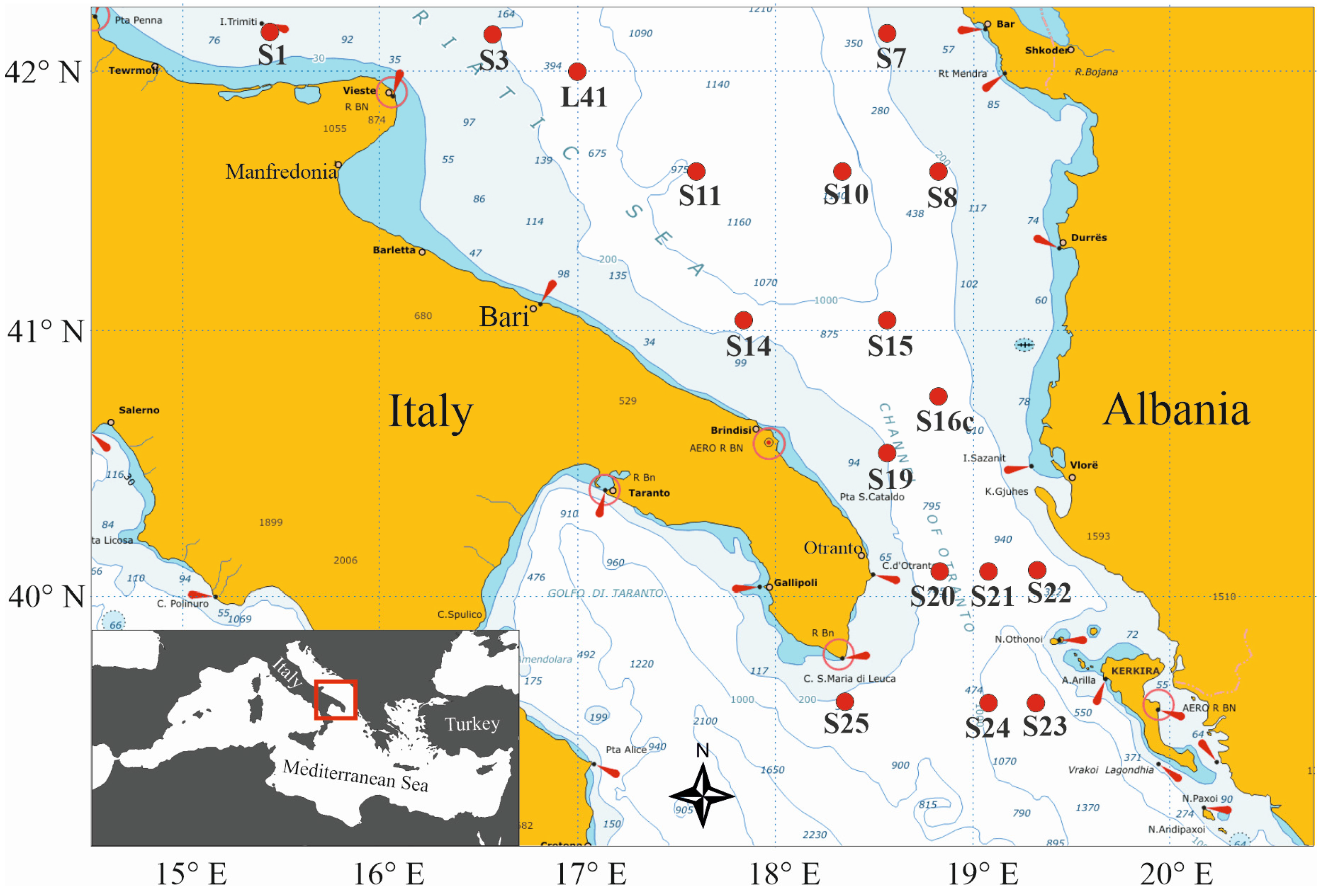
2.1. Study Area
2.2. Sampling Procedure
2.3. Laboratory Zooplankton Analysis
2.4. Identification of Diel Patterns
2.5. Statistical Analysis
3. Results
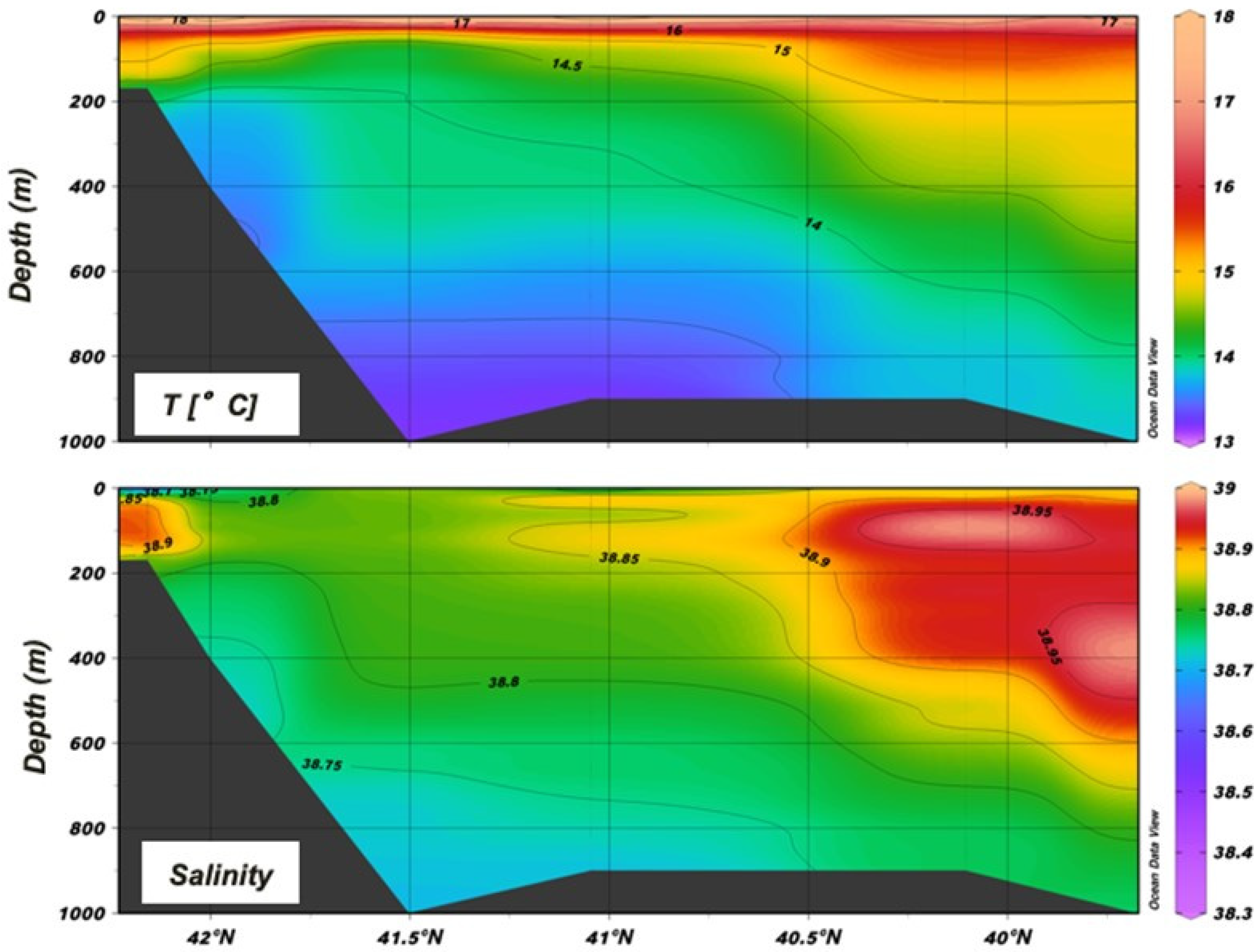
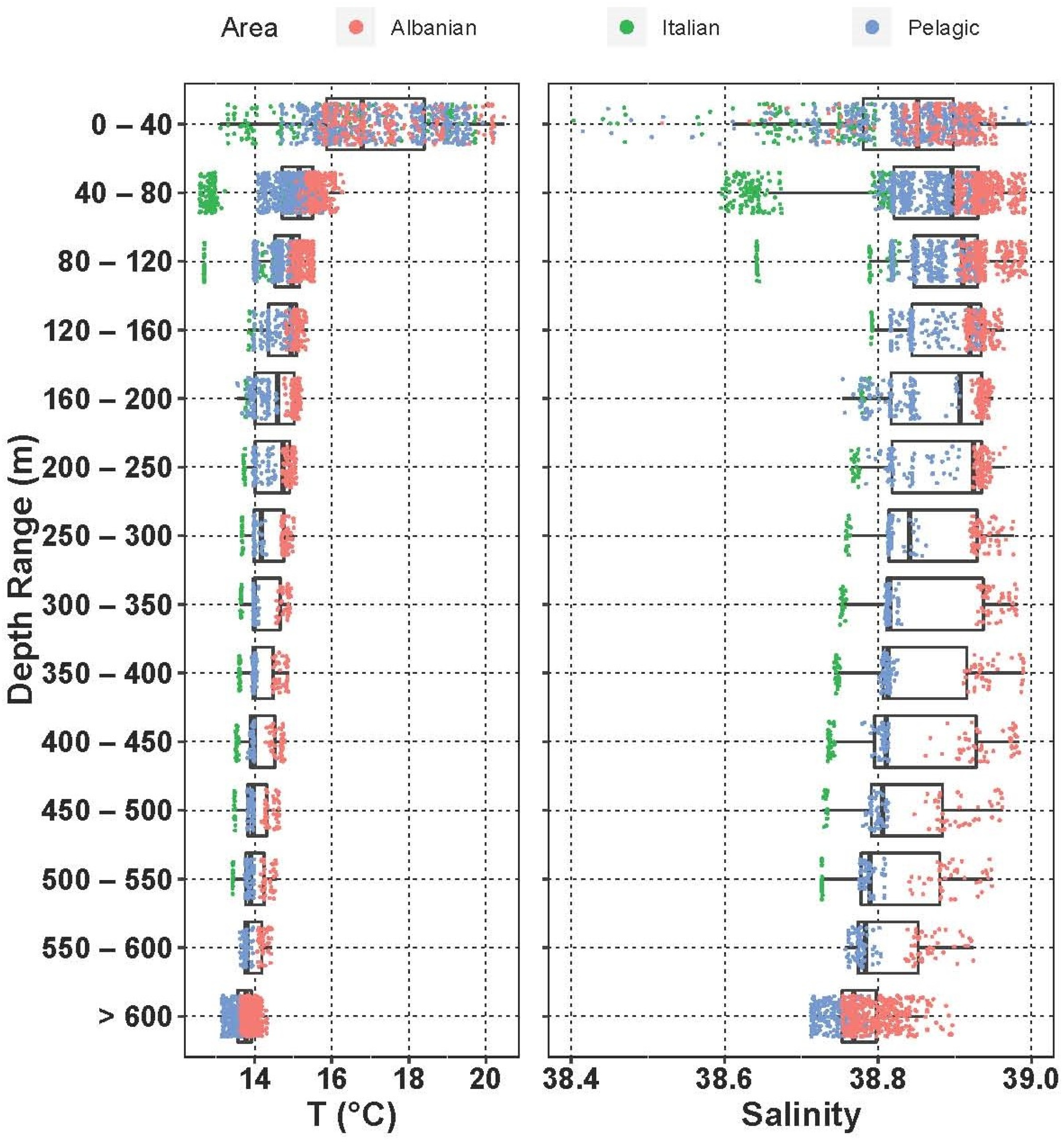
3.1. Oceanographic Conditions
3.2. Zooplankton
3.3. Fish Larvae
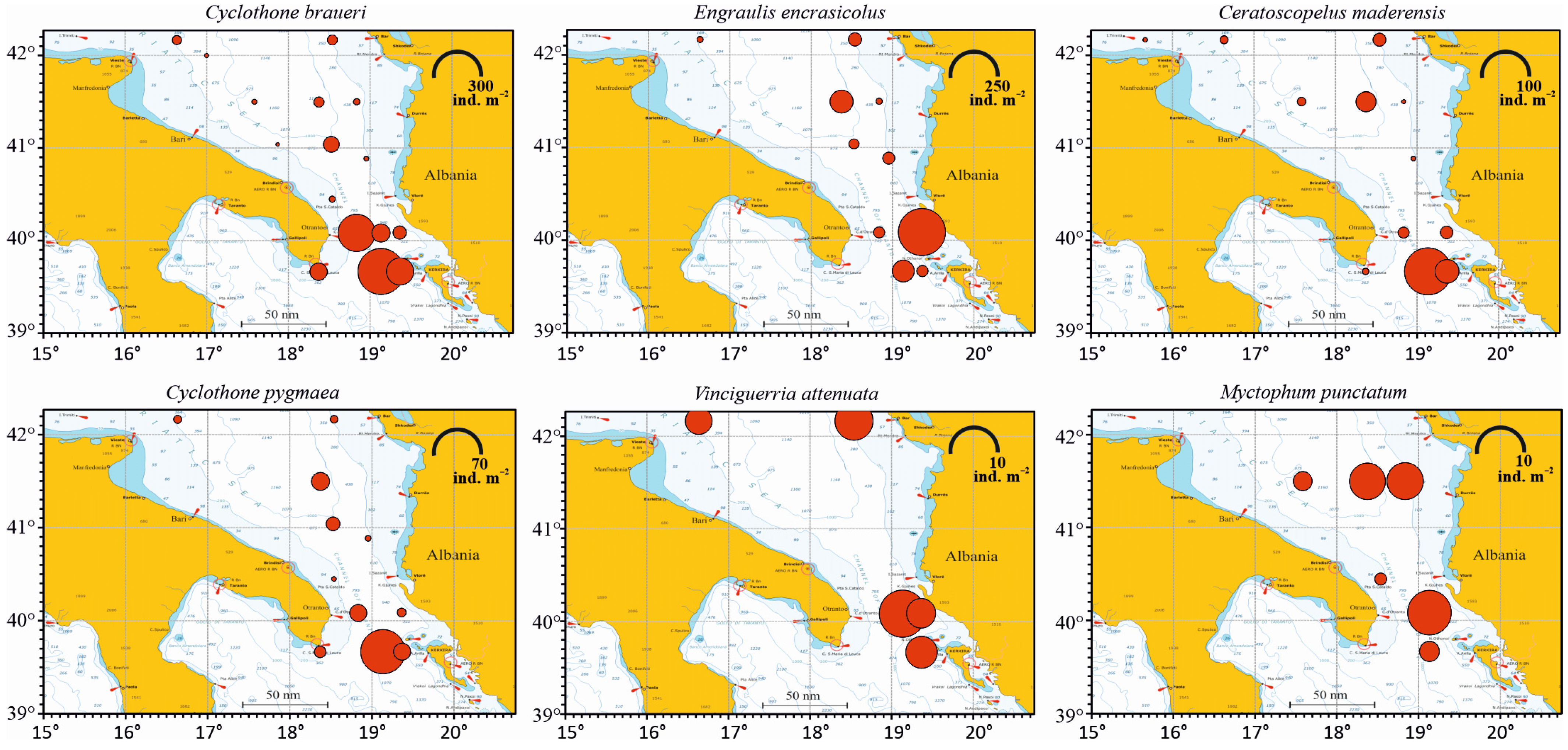
3.3.1. Composition
3.3.2. Horizontal Distribution
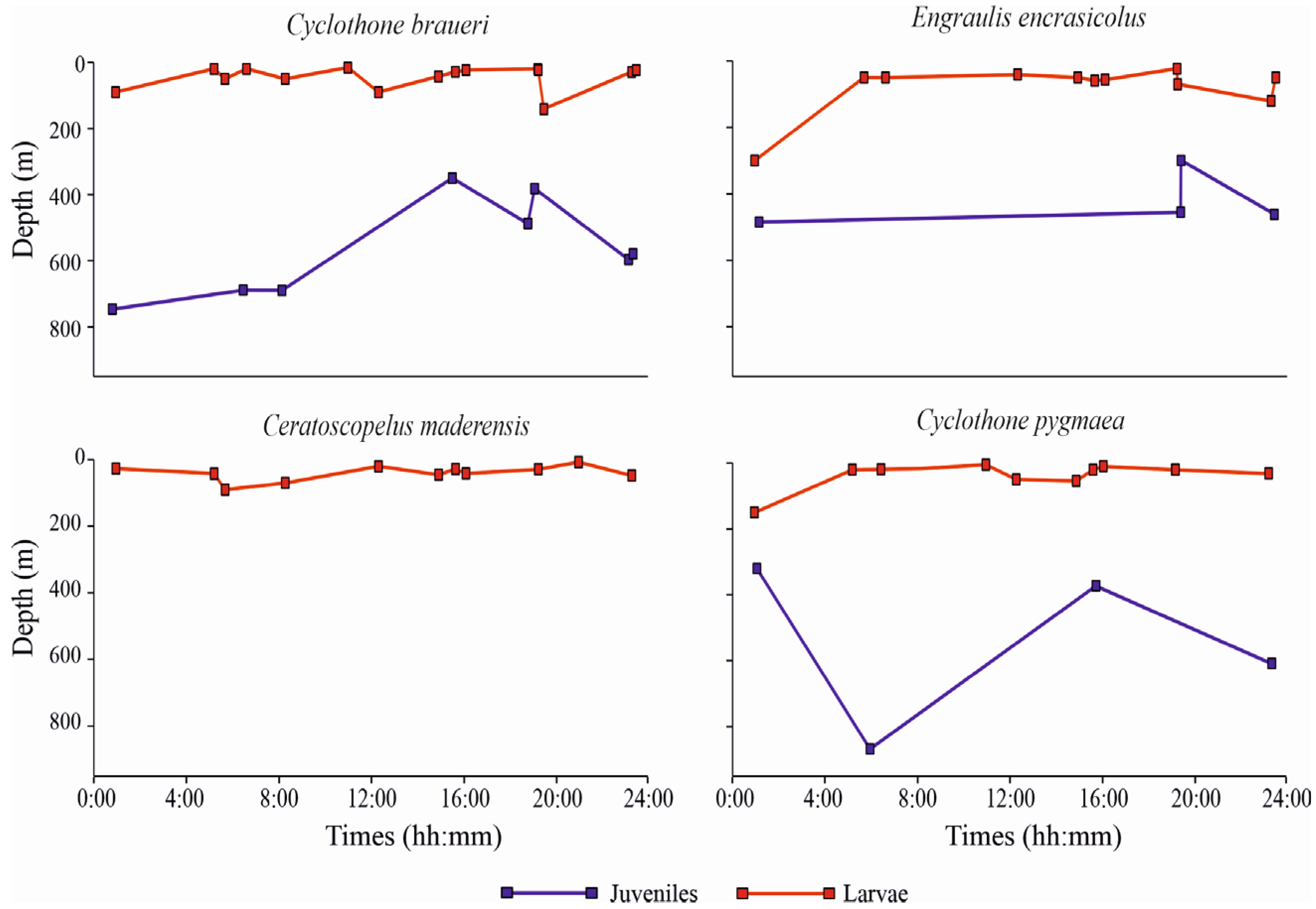
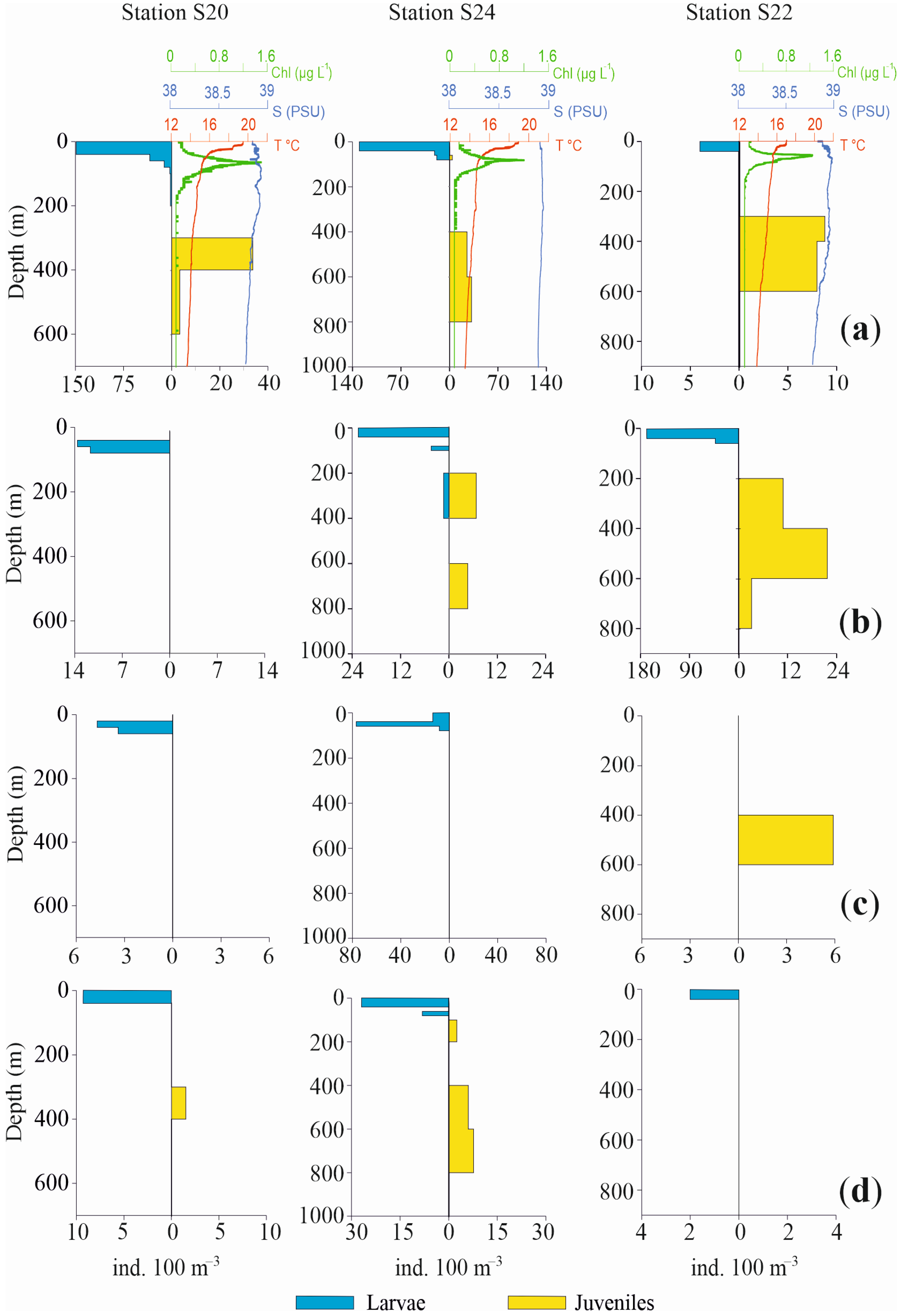
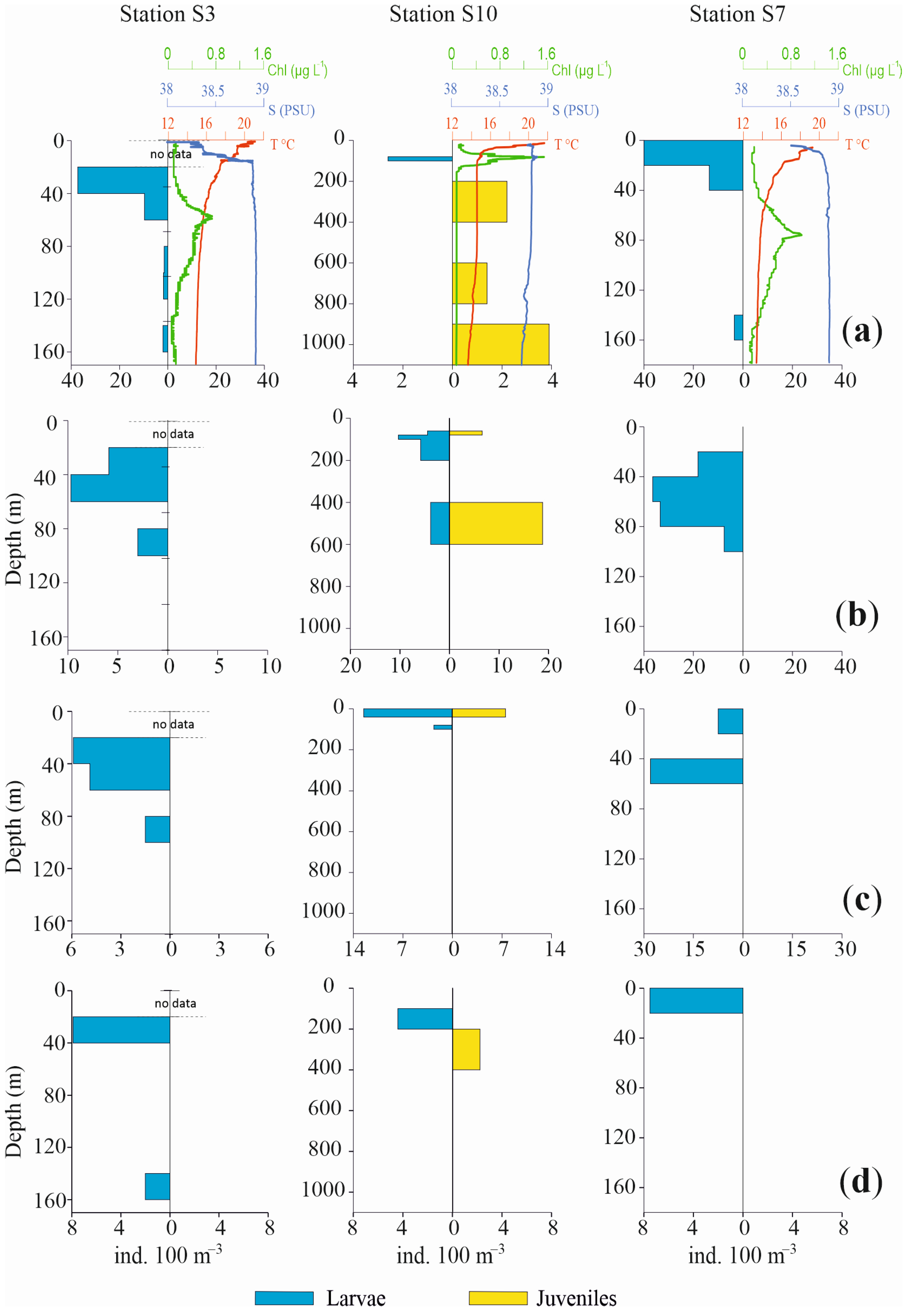
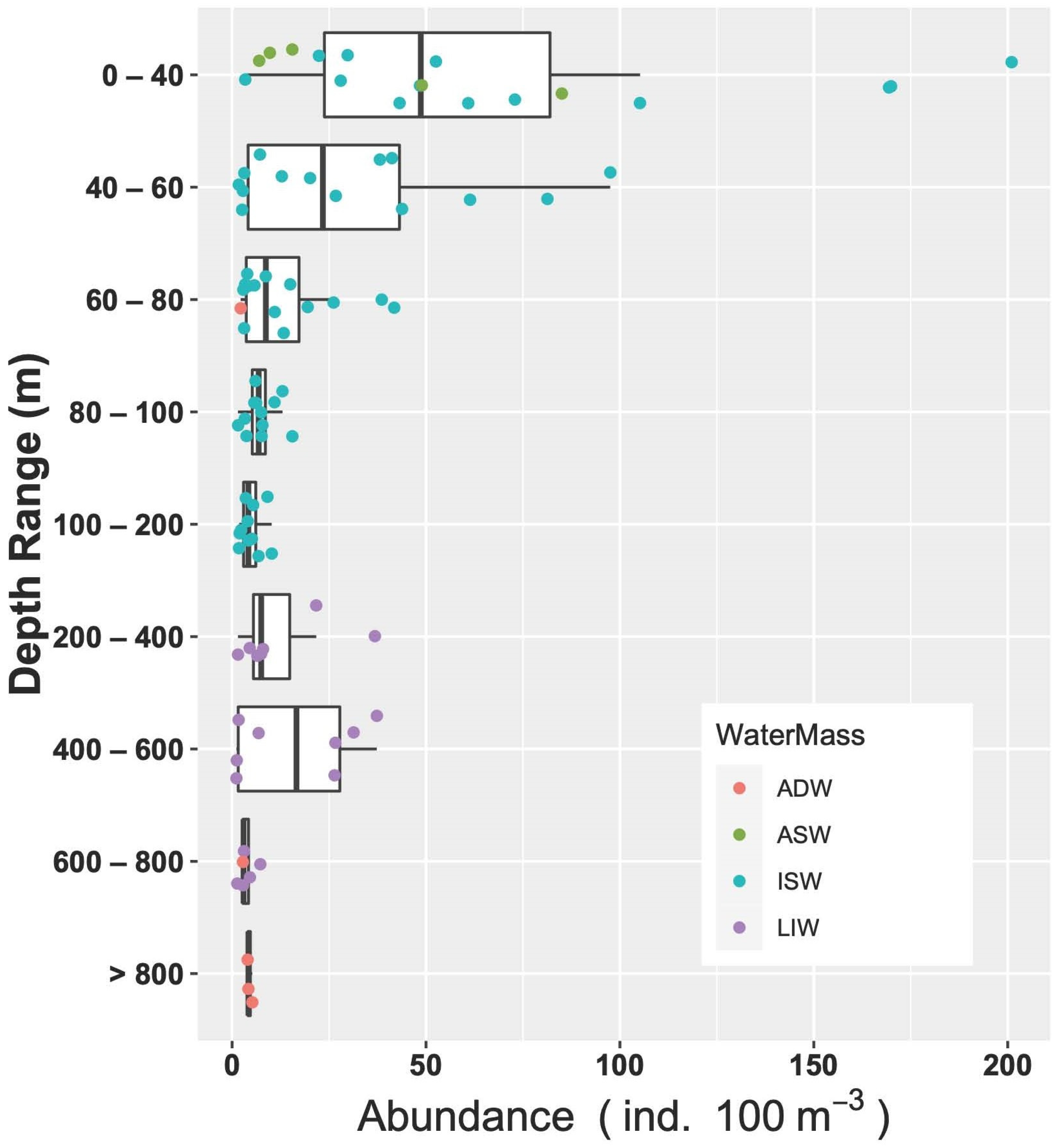
3.3.3. Vertical Distribution
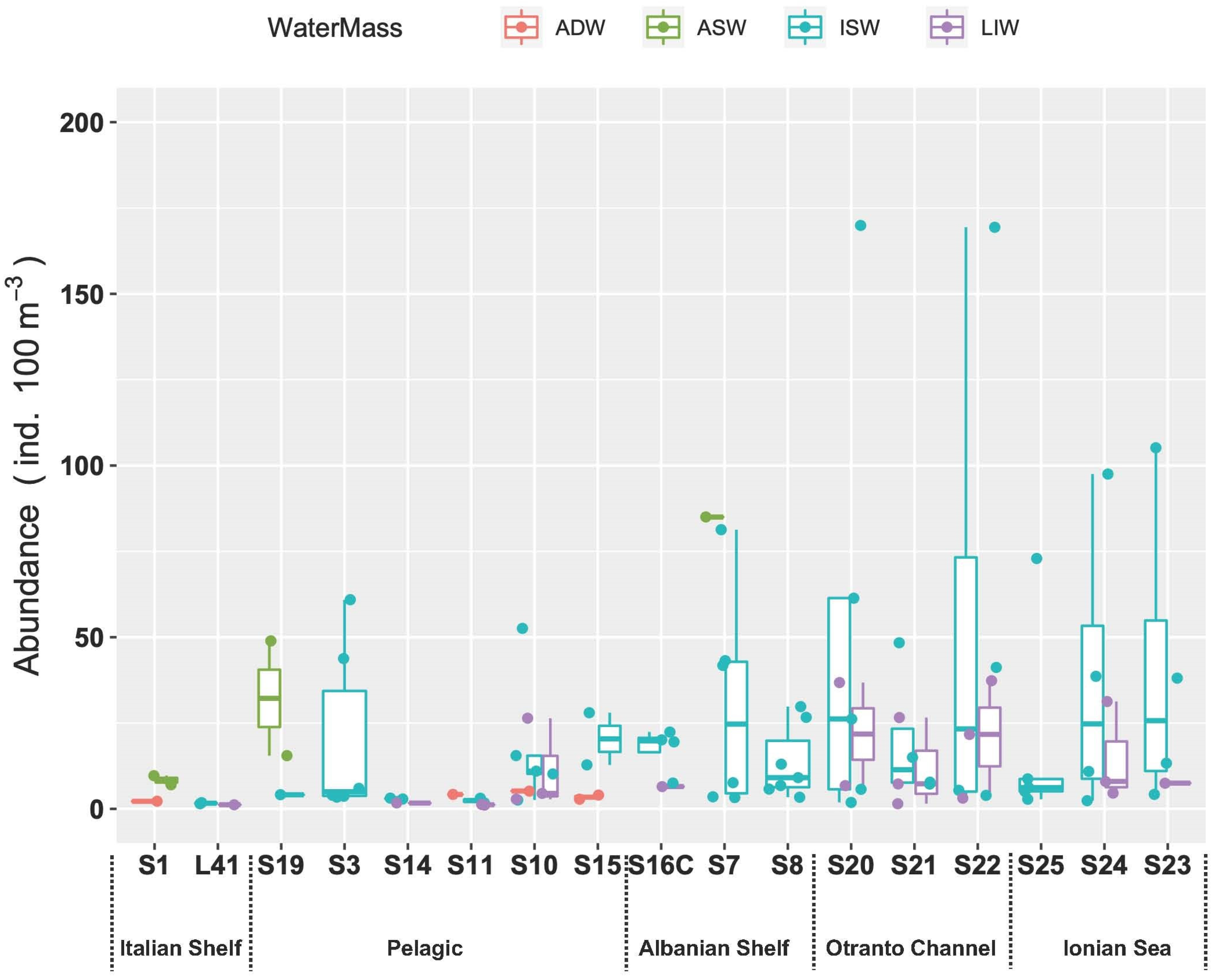
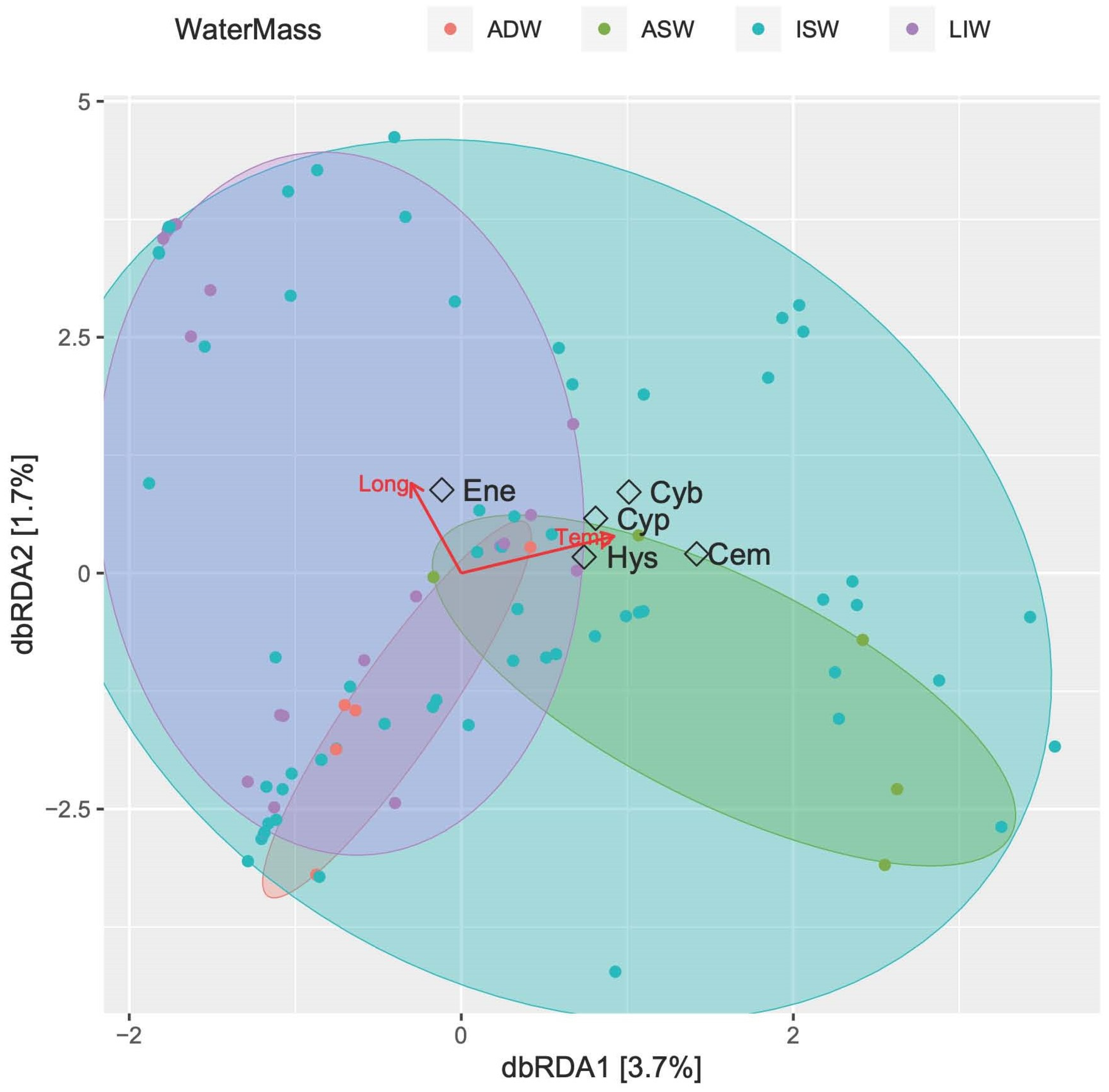
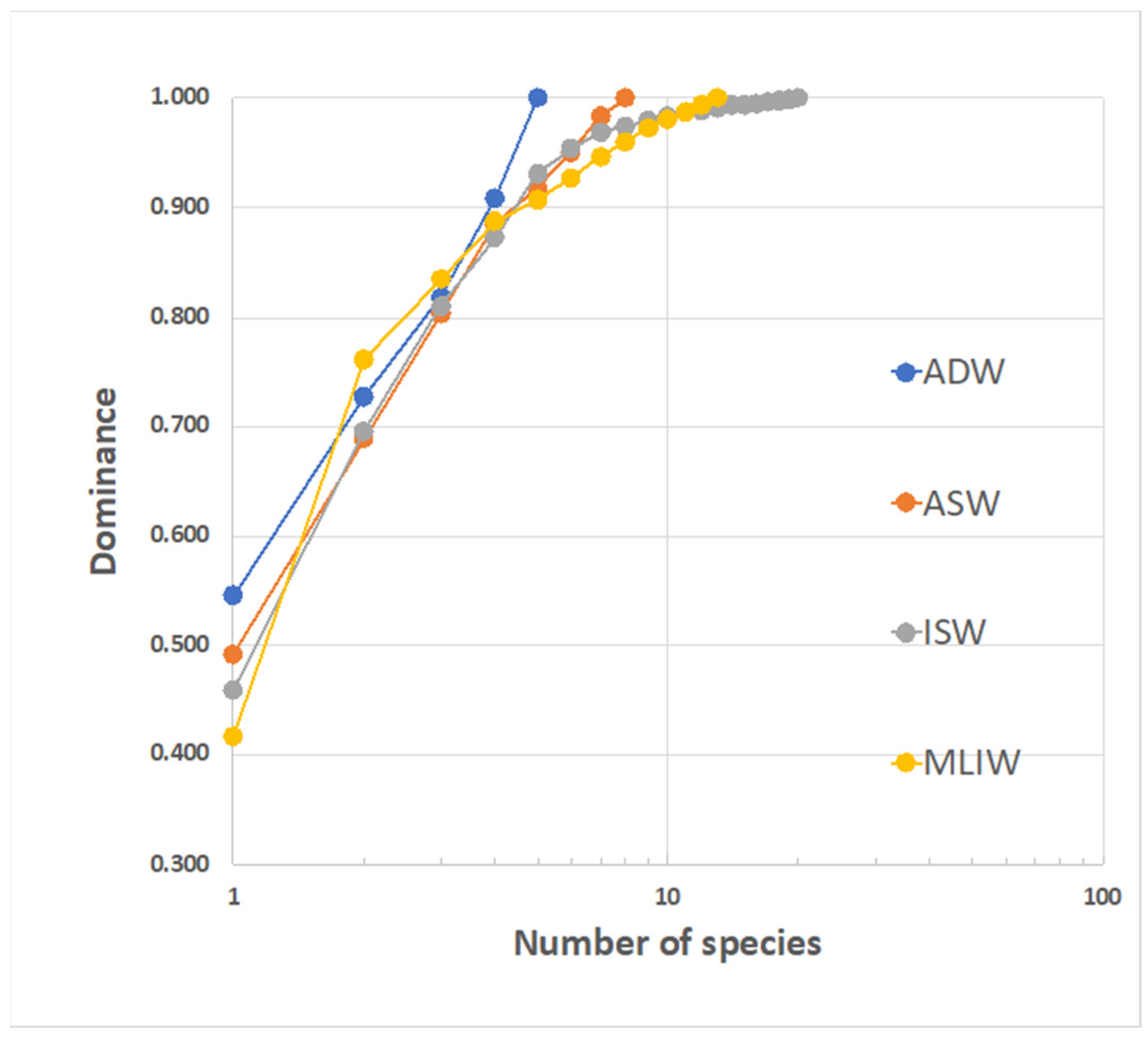
3.3.4. Fish Larvae Abundance and Biodiversity Relationship with Water Masses
4. Discussion
5. Conclusions
Supplementary Materials
Author Contributions
Funding
Data Availability Statement
Acknowledgments
Conflicts of Interest
References
- Sabatés, A.; Olivar, M.P.; Salat, J.; Palomera, I.; Alemany, F. Physical and biological processes controlling the distribution of fish larvae in the NW Mediterranean. Progr. Oceanogr. 2007, 74, 355–376. [Google Scholar] [CrossRef]
- Espinosa-Fuentes, M.L.; Flores-Coto, C. Cross-shelf and vertical structure of ichthyoplankton assemblages in continental shelf waters of the Southern Gulf of Mexico. Estuar. Coast. Shelf Sci. 2004, 59, 333–352. [Google Scholar] [CrossRef]
- Richards, W.J. Early Stages of Atlantic Fishes: An Identification Guide for the Western Central North Atlantic; CRC Press: Boca Raton, FL, USA, 2006. [Google Scholar]
- Gonzalo, D.B.; Jiménez-Rosenberg, S.P.A.; Echeverri-García, L.d.P.; Fernández-Álamo, M.A.; Ordóñez-López, U.; Herzka, S.Z. Distribution and densities of fish larvae species with contrasting life histories as a function of oceanographic variables in the deep-water region of the southern Gulf of Mexico. PLoS ONE 2023, 18, e0280422. [Google Scholar] [CrossRef]
- Martínez-López, B.; Zavala-Hidalgo, J. Seasonal and interannual variability of cross-shelf transports of chlorophyll in the Gulf of Mexico. J. Mar. Syst. 2009, 77, 1–20. [Google Scholar] [CrossRef]
- Otis, D.B.; Le Hénaff, M.; Kourafalou, V.H.; McEachron, L.; Muller-Karger, F.E. Mississippi River and Campeche Bank (Gulf of Mexico) episodes of cross-shelf export of coastal waters observed with satellites. Remote Sens. 2019, 11, 723. [Google Scholar] [CrossRef]
- Compaire, J.C.; Perez-Brunius, P.; Jiménez-Rosenberg, S.P.A.; Rodríguez Outeruelo, J.; Echeverri-García, L.P.; Herzka, S.Z. Connectivity of coastal and neritic fish larvae to the deep waters. Limnol. Oceanogr. 2021, 66, 2423–2441. [Google Scholar] [CrossRef]
- Froese, R.; Pauly, D. FishBase. World Wide Web Electronic Publication. Version December 2021. Available online: http://www.fishbase.org/ (accessed on 12 June 2023).
- Patti, B.; Torri, M.; Cuttitta, A. General surface circulation controls the interannual fluctuations of anchovy stock biomass in the central Mediterranean Sea. Sci. Rep. 2020, 10, 1554. [Google Scholar] [CrossRef]
- Patti, B.; Torri, M.; Cuttitta, A. Interannual summer biodiversity changes in ichthyoplankton assemblages of the Strait of Sicily (Central Mediterranean) over the period 2001–2016. Front. Mar. Sci. 2022, 9, 960929. [Google Scholar] [CrossRef]
- Nonaka, R.H.; Matsuura, Y.; Suzuki, K. Seasonal variation in larval fish assemblages in relation to oceanographic conditions in the abrolhos bank region off eastern Brazil. Fish. Bull. 2000, 98, 767–784. [Google Scholar]
- Koutrakis, E.T.; Kallianiotis, A.A.; Tsikiliras, A.C. Temporal pattern of larval fish distribution and abundance in a coastal area of northern Greece. Sci. Mar. 2004, 68, 585–595. [Google Scholar] [CrossRef]
- Palomera, I.; Olivar, M.P.; Morales-Nin, B. Larval development and growth of the European hake Merluccius merluccius in the northwestern Mediterranean. Sci. Mar. 2005, 69, 251–258. [Google Scholar] [CrossRef]
- Giordano, D.; Profeta, A.; Busalacchi, B.; Minutoli, R.; Guglielmo, L.; Bergamasco, A.; Granata, A. Summer larval fish assemblages in the Southern Tyrrhenian Sea (Western Mediterranean Sea). Mar. Ecol. 2015, 36, 104–117. [Google Scholar] [CrossRef]
- Neilson, J.D.; Perry, R.I. Diel vertical migrations of marine fishes: An obligate or facultative process? Adv. Mar. Biol. 1990, 26, 115–168. [Google Scholar]
- Heath, M.R. Field investigations of the early life-history stages of marine fish. Adv. Mar. Biol. 1992, 28, 2–174. [Google Scholar]
- Somarakis, S.; Drakopoulos, P.G.; Filippou, V. Distribution and abundance of larval fish in the Northern Aegean Sea–Eastern Mediterranean–in relation to early summer oceanographic conditions. J. Plankton Res. 2002, 24, 339–357. [Google Scholar] [CrossRef]
- Gray, C.A. Do thermoclines explain the vertical distributions of larval fishes in the dynamic coastal waters of southeastern Australia? J. Mar. Fresh. Res. 1996, 47, 183–190. [Google Scholar] [CrossRef]
- Conway, D.V.P.; Coombs, S.H.; Smith, C. Feeding of anchovy Engraulis encrasicolus larvae in the northwestern Adriatic Sea in response to changing hydrobiological conditions. Mar. Ecol. Prog. Ser. 1998, 175, 35–49. [Google Scholar] [CrossRef]
- Granata, A.; Bergamasco, A.; Battaglia, P.; Milisenda, G.; Pansera, M.; Bonanzinga, V.; Arena, G.; Greco, S.; Guglielmo, R.; Spanò, N.; et al. Vertical distribution and diel migration of zooplankton and micronekton in Polcevera submarine canyon of the Ligurian mesopelagic zone (NW Mediterranean Sea). Progr. Oceanogr. 2020, 183, 102298. [Google Scholar] [CrossRef]
- Richards, T.M.; Sutton, T.T.; Wells, R.J.D. Trophic structure and sources of variation influencing the stable isotope signatures of meso- and bathypelagic micronekton fishes. Front. Mar. Sci. 2020, 7, 507992. [Google Scholar] [CrossRef]
- Isari, S.; Fragopoulu, N.; Somarakis, S. Interannual variability in horizontal patterns of larval fish assemblages in the northeastern Aegean Sea (eastern Mediterranean) during early summer. Estuar. Coast. Shelf Sci. 2008, 79, 607–619. [Google Scholar] [CrossRef]
- Gačić, M.; Civitarese, G.; Ursella, L. Spatial and seasonal variability of water and biogeochemical fuxes in the Adriatic Sea. In The Eastern Mediterranean as A Laboratory Basin for the Assessment of Contrasting Ecosystems; Kluwer Academic Publisher: Dordrecht, The Netherlands, 1999; pp. 335–357. [Google Scholar]
- Gačić, M.; Kovačević, V.; Manca, B.; Papageorgiou, E.; Poulain, P.M.; Scarazzato, P.; Vetrano, A. Thermohaline properties and circulation in the Strait of Otranto. In Dynamics of Mediterranean Straits and Channels; CIESM Science Series; Bulletin de L’Institut Ocea11ographique, n° Special 17; Musée Océanographique: Monaco City, Monaco, 1996; pp. 117–145. [Google Scholar]
- Manca, B.B.; Scarazzato, P. The two regimes of the intermediate/deep circulation in the Ionian-Adriatic Seas. Arch. Oceanogr. Linol. 2001, 22, 15–26. [Google Scholar]
- Bignami, F.; Salusti, E.; Schiarini, S. Observations on a bottom vein of dense water in the Southern Adriatic and Ionian Seas. J. Geophys. Res. 1990, 95, 7249–7259. [Google Scholar] [CrossRef]
- Sameoto, D.D.; Jaroszyski, L.O.; Fraser, W.B. BIONESS, a new design in multiple net zooplankton samplers. Can. J. Fish Aquat. Sci. 1980, 37, 722–724. [Google Scholar] [CrossRef]
- Barange, M. Vertical migration and habitat partitioning of six euphausiid species in the northern Benguela upwelling system. J. Plankton Res. 1990, 12, 1123–1223. [Google Scholar] [CrossRef]
- Andersen, V.; Sardou, J. The diel migrations and vertical distributions of zooplankton and micronekton in the Northwestern Mediterranean Sea. 1. Euphausiids, mysids, decapods and fishes. J. Plankton Res. 1992, 14, 1129–1154. [Google Scholar] [CrossRef]
- Guglielmo, R.; Bergamasco, A.; Minutoli, R.; Patti, F.P.; Belmonte, G.; Spanò, N.; Zagami, G.; Bonanzinga, V.; Guglielmo, L.; Granata, A. The Otranto Channel (South Adriatic Sea), a hot-spot area of plankton biodiversity: Pelagic polychaetes. Sci. Rep. 2019, 9, 19490. [Google Scholar] [CrossRef] [PubMed]
- Frederiksen, M.; Edwards, M.; Richardson, A.J.; Halliday, N.C.; Wanless, S. From plankton to top predators: Bottom-up control of a marine food web across four trophic levels. J. Anim. Ecol. 2006, 75, 1259–1268. [Google Scholar] [CrossRef]
- Rothschild, B.J. “Fish stocks and recruitment”: The past thirty years. ICES J. Mar. Sci. 2000, 57, 191–201. [Google Scholar] [CrossRef]
- Miller, T.J. Contribution of individual-based coupled physical-biological models to understanding recruitment in marine fish populations. Mar. Ecol. Prog. Ser. 2007, 347, 127–138. [Google Scholar] [CrossRef]
- Cowen, R.K.; Sponaugle, S. Larval Dispersal and Marine Population Connectivity. Ann. Rev. Mar. Sci. 2009, 1, 443–466. [Google Scholar] [CrossRef]
- Bruno, R.; Granata, A.; Cefali, A.; Guglielmo, L.; Brancato, G.; Barbera, P. Relationship between fish larvae biomass and plankton production in the south Tyrrhenian Sea. In Mediterranean Ecosystems Structures and Processes; Faranda, F.M., Guglielmo, L., Spezie, G., Eds.; Springer: Milan, Italy, 2001. [Google Scholar]
- Fuiman, L.A.; Davis, R.W.; Williams, T.M. Behavior of midwater fishes under the Antarctic ice: Observations by a predator. Mar. Biol. 2002, 140, 815–822. [Google Scholar]
- De Mitcheson, Y.S.; Erisman, B.E. Reef Fish Spawning Aggregations: Biology, Research and Management; Springer: Berlin/Heidelberg, Germany, 2012. [Google Scholar] [CrossRef]
- Lindo-Atichati, D.; Bringas, F.; Goni, G.J.; Muhling, B.A.; Muller-Karger, F.E.; Habtes, S. Varying mesoscale structures influence larval fish distribution in the northern Gulf of Mexico. Mar. Ecol. Prog. Ser. 2012, 463, 245–257. [Google Scholar] [CrossRef]
- Rooker, J.R.; Kitchens, L.L.; Dance, M.A.; Wells, R.J.D.; Falterman, B.; Cornic, M. Spatial, Temporal, and Habitat-Related Variation in Abundance of Pelagic Fishes in the Gulf of Mexico: Potential Implications of the Deepwater Horizon Oil Spill. PLoS ONE 2013, 8, e76080. [Google Scholar] [CrossRef] [PubMed]
- Brogan, M.W. Two methods of sampling fish larvae over reefs: A comparison from the Gulf of California. Mar. Biol. 1994, 118, 33–44. [Google Scholar] [CrossRef]
- Sponaugle, S.; Cowen, R.K.; Shanks, A.L.; Morgan, S.G.; Fortier, J.; Pineda, J.; Boehlert, G.; Kingsford, M.J.; Lindeman, K.; Grimes, C.; et al. Predicting self-recruitment in marine populations: Biophysical correlates and mechanisms. Bull. Mar. Sci. 2002, 49, 341–375. [Google Scholar]
- Hedberg, P.; Rybak, F.F.; Gullström, M.; Jiddawi, N.S.; Winder, M. Fish larvae distribution among different habitats in coastal East Africa. J. Fish Biol. 2019, 94, 29–39. [Google Scholar] [CrossRef] [PubMed]
- Irisson, J.O.; Paris, C.B.; Guigand, C.; Planes, S. Vertical distribution and ontogenetic “migration” in coral reef fish larvae. Limnol. Oceanogr. 2010, 55, 909–919. [Google Scholar] [CrossRef]
- Olivar, M.P.; Bernal, A.; Molí, B.; Peña, M.; Balbín, R.; Castellón, A.; Miguel, J.; Massuti, E. Vertical distribution, diversity and assemblages of mesopelagic fishes in the western Mediterranean. Deep. Sea Res. Part I Oceanogr. Res. Pap. 2012, 62, 53–69. [Google Scholar] [CrossRef]
- Andersen, V.; François, F.; Sardou, J.; Picheral, M.; Scotto, M.; Nival, P. Vertical distributions of macroplankton and micronekton in the Ligurian and Tyrrhenian Seas (northwestern Mediterranean). Oceanol. Acta 1998, 21, 655–676. [Google Scholar] [CrossRef]
- Bernal, A.; Olivar, M.P.; Maynou, F.; de Puelles, M.L.F. Diet and feeding strategies of mesopelagic fishes in the western Mediterranean. Progr. Oceanogr. 2015, 135, 1–17. [Google Scholar] [CrossRef]
- Granata, A.; Cubeta, A.; Minutoli, R.; Bergamasco, A.; Guglielmo, L. Distribution and abundance of fish larvae in the northern Ionian Sea (Eastern Mediterranean). Helg. Mar. Res. 2011, 65, 381–398. [Google Scholar] [CrossRef]
- Cuttitta, A.; Torri, M.; Zarrad, R.; Zgozi, S.; Jarboui, O.; Quinci, E.M.; Amza, M.M.; Elfituri, A.; Haddoud, D.; El Turki, A.; et al. Linking surface hydrodynamics to planktonic ecosystem: The case study of the ichthyoplanktonic assemblages in the Central Mediterranean Sea. Hydrobiologia 2018, 821, 191–214. [Google Scholar] [CrossRef]
- Battaglia, P.; Ammendolia, G.; Cavallaro, M.; Consoli, P.; Esposito, V.; Malara, D.; Rao, I.; Romeo, T.; Andaloro, F. Influence of lunar phases, winds and seasonality on the stranding of mesopelagic fish in the Strait of Messina (Central Mediterranean Sea). Mar. Ecol. 2017, 38, e12459. [Google Scholar] [CrossRef]
- Granata, A.; Bergamasco, A.; Zagami, G.; Guglielmo, R.; Bonanzinga, V.; Minutoli, R.; Geraci, A.; Pagano, L.; Swadling, K.; Battaglia, P.; et al. Daily vertical distribution and diet of Cyclothone braueri (Gonostomatidae) in the Polcevera submarine canyon (Ligurian Sea, north-western Mediterranean). Deep Sea Res. 2023, 199, 104113. [Google Scholar] [CrossRef]
- Badcock, J. Gonostomatidae. In Fishes of the North-Eastern Atlantic and the Mediterranean; Whitehead, P.J.P., Bauchot, M.L., Hureau, J.C., Nielsen, J., Tortonese, E., Eds.; Unesco: Paris, France, 1984; Volume 1, pp. 284–301. [Google Scholar]
- Ariza, A.; Landeira, J.M.; Escanez, A.; Wienerroither, R.; Aguilar de Soto, N.; Røstad, A.; Kaartvedt, S.; Hernández-León, S. Vertical distribution, composition and migratory patterns of acoustic scattering layers in the Canary Islands. J. Mar. Syst. 2016, 157, 82–91. [Google Scholar] [CrossRef]
- Maso, M.; Palomera, I. Vertical distribution of midwater fish larvae off Western Mediterranean. Inv. Pesq. 1984, 48, 455–468. [Google Scholar]
- Torri, M.; Pappalardo, A.M.; Ferrito, V.; Giannì, S.; Armeri, G.M.; Patti, C.; Mangiaracina, F.; Biondo, G.; Di Natale, M.; Musco, M.; et al. Signals from the deep-sea: Genetic structure, morphometric analysis, and ecological implications of Cyclothone braueri (Pisces, Gonostomatidae) early life stages in the Central Mediterranean Sea. Mar. Environ. Res. 2021, 169, 105379. [Google Scholar] [CrossRef]
- John, H.C. Horizontal, vertical distribution of lancelet larvae, fish larvae in the Sargasso Sea during spring 1979. Meeresforsch 1984, 31, 133–143. [Google Scholar]
- Sabatés, A.; Masò, M. Effect of a shelf slope front on the spatial distribution of mesopelagic fish larvae in the western Mediterranean. Deep Sea Res. 1990, 37, 1085–1098. [Google Scholar] [CrossRef]
- Olivar, M.P.; Beckley, L.E. Influence of the Agulhas current on the distribution of lanternfish larvae off the southeast coast of Africa. J. Plankton Res. 1994, 16, 1759–1780. [Google Scholar] [CrossRef]
- Olivar, M.P.; Palomera, I. Ontogeny and distribution of Hygophum benoiti (Pisces Myctophidae) of the western Mediterranean. J. Plankton Res. 1994, 16, 977–991. [Google Scholar] [CrossRef]
- Sabatés, A. Distribution pattern of larval fish populations in the Northwestern Mediterranean. Mar. Ecol. Prog. Ser. 1990, 59, 75–82. [Google Scholar] [CrossRef]
- Le Févre, J. Aspects of the biology of frontal systems. Adv. Mar. Biol. 1986, 23, 163–299. [Google Scholar]
- Gorelova, T.A. A quantitative assessment of consumption of zooplankton by epipelagic lanternfishes (Family Myctophidae) in the equatorial Pacific Ocean. J. Ichthyol. 1983, 23, 106–113. [Google Scholar]
- Dalpadado, P.; Gjøsaeter, J. Feeding ecology of the lanternfish Benthosema pterotum from the Indian Ocean. Mar. Biol. 1988, 99, 555–567. [Google Scholar] [CrossRef]
- Battaglia, P.; Pagano, L.; Consoli, P.; Esposito, V.; Granata, A.; Guglielmo, L.; Pedà, C.; Romeo, T.; Zagami, G.; Vicchi, T.E.; et al. Consumption of mesopelagic prey in the Strait of Messina, an upwelling area of the central Mediterranean Sea: Feeding behaviour of the blue jack mackerel Trachurus picturatus (Bowdich, 1825). Deep. Sea Res. Part I Oceanogr. Res. Pap. 2020, 155, 103158. [Google Scholar] [CrossRef]
- Watanabe, H.; Kawaguchi, K.; Hayashi, A. Feeding habits of juvenile surface-migratory myctophid fishes (family Myctophidae) in the Kuroshio region of the western North Pacific. Mar. Ecol. Prog. Ser. 2002, 236, 263–272. [Google Scholar] [CrossRef]
- D’Elia, M.; Warren, J.D.; Rodriguez-Pinto, I.; Sutton, T.T.; Cook, A.; Boswell, K.M. Diel variation in the vertical distribution of deep-water scattering layers in the Gulf of Mexico. Deep. Sea Res. Part I Oceanogr. Res. Pap. 2016, 115, 91–102. [Google Scholar] [CrossRef]

| Station | Local Date | Position | Local Time | Bottom Depth | Max Sampled Depth | No. of Samples | ||
|---|---|---|---|---|---|---|---|---|
| Lat. N | Long. E | Start | End | (m) | (m) | |||
| S1 | 9-May-2013 | 42°09.994′ | 15°39.966′ | 20:23 | 21:37 | 99 | 90 | 9 |
| L41 | 10-May-2013 | 41°59.952′ | 16°59.872′ | 18:38 | 20:21 | 580 | 550 | 9 |
| S3 | 10-May-2013 | 42°09.985′ | 16°38.059′ | 14:05 | 15:47 | 178 | 170 | 8 |
| S10 | 11-May-2013 | 41°29.780′ | 18°22.453′ | 23:48 | 02:07 | 1123 | 1096 | 9 |
| S7 | 11-May-2013 | 42°10.049′ | 18°32.310′ | 15:28 | 16:46 | 190 | 180 | 9 |
| S8 | 12-May-2013 | 41°29.971′ | 18°50.127′ | 04:47 | 06:35 | 324 | 310 | 9 |
| S16c | 13-May-2013 | 40°53.072′ | 18°57.210′ | 11:48 | 13:09 | 317 | 300 | 8 |
| S15 | 13-May-2013 | 41°02.365′ | 18°31.554′ | 05:36 | 07:38 | 939 | 900 | 8 |
| S22 | 14-May-2013 | 40°05.222′ | 19°21.708′ | 18:03 | 20:25 | 965 | 900 | 9 |
| S21 | 14-May-2013 | 40°05.008′ | 19°08.001′ | 22:17 | 00:28 | 972 | 900 | 8 |
| S23 | 15-May-2013 | 39°40.001′ | 19°22.009′ | 18:01 | 20:29 | 1172 | 1100 | 9 |
| S24 | 15-May-2013 | 39°40.004′ | 19°08.008′ | 22:14 | 00:23 | 1089 | 1000 | 9 |
| S20 | 16-May-2013 | 40°05.012′ | 18°50.071′ | 14:50 | 16:41 | 738 | 700 | 9 |
| S25 | 16-May-2013 | 39°39.917′ | 18°22.140′ | 04:26 | 05:59 | 261 | 210 | 8 |
| S19 | 17-May-2013 | 40°26.801′ | 18°32.195′ | 10:19 | 11:42 | 127 | 100 | 7 |
| S14 | 17-May-2013 | 41°02.305′ | 17°52.030′ | 18:02 | 19:51 | 699 | 600 | 9 |
| S11 | 18-May-2013 | 41°29.991′ | 17°34.972′ | 07:10 | 09:25 | 1137 | 1060 | 9 |
| Family/Species | N | Relative Abundance | Frequency | Mean Abundance |
|---|---|---|---|---|
| (%) | (%) | (ind. m−2) | ||
| Carangidae | ||||
| Trachurus trachurus | 1 | 0.09 | 5.88 | 0.04 |
| Cepolidae | ||||
| Cepola rubescens | 6 | 0.53 | 23.53 | 0.41 |
| Engraulidae | ||||
| Engraulis encrasicolus | 268 | 23.59 | 64.71 | 27.58 |
| Gonostomatidae | ||||
| Cyclothone braueri | 518 | 45.60 | 94.12 | 45.40 |
| Cyclothone pygmaea | 71 | 6.25 | 64.71 | 6.28 |
| Cyclothone sp. | 6 | 0.53 | 11.76 | 0.37 |
| Labridae | ||||
| Coris julis | 4 | 0.35 | 11.76 | 0.40 |
| Myctophidae | ||||
| Benthosema glaciale | 2 | 0.18 | 5.88 | 0.21 |
| Diaphus holti | 1 | 0.09 | 5.88 | 0.14 |
| Ceratoscopelus maderensis | 115 | 10.12 | 70.59 | 10.16 |
| Hygophum benoiti | 5 | 0.44 | 17.65 | 0.34 |
| Hygophum sp. | 55 | 4.84 | 70.59 | 3.95 |
| Lampanictus pusillus | 1 | 0.09 | 5.88 | 0.14 |
| Lampanictus crocodilus | 3 | 0.26 | 11.76 | 0.30 |
| Lobianchia sp. | 1 | 0.09 | 5.88 | 0.11 |
| Myctophum punctatum | 18 | 1.58 | 35.29 | 1.47 |
| Paralepitidae | ||||
| Paralepis speciosa | 1 | 0.09 | 5.88 | 0.12 |
| Photychthaidae | ||||
| Vinciguerria attenuata | 33 | 2.90 | 29.41 | 1.98 |
| Vinciguerria sp. | 12 | 1.06 | 17.65 | 1.89 |
| Pomacentridae | ||||
| Chromis chromis | 2 | 0.18 | 11.76 | 0.22 |
| Serranidae | ||||
| Serranus sp. | 2 | 0.18 | 5.88 | 0.03 |
| Sgombridae | ||||
| Auxis rochei | 5 | 0.44 | 17.65 | 0.50 |
| Thunnus thynnus | 1 | 0.09 | 5.88 | 0.11 |
| Sternoptychidae | ||||
| Argyropelecus hemigymnus | 2 | 0.18 | 5.88 | 0.11 |
| Stomiidae | ||||
| Chauliodus sloani | 1 | 0.09 | 5.88 | 0.17 |
| Unidentified specimens | 2 | 0.18 | 11.76 | 0.16 |
| Water Mass | No. of Specimens | Species Richness | Margalef Index | Alpha Diversity | Whittaker’ Species Turnover |
|---|---|---|---|---|---|
| ASW | 61 | 8 | 1.7 | 2.4 | 2.3 |
| ISW | 913 | 20 | 2.78 | 2.06 | 8.7 |
| MLIW | 151 | 13 | 2.39 | 1.75 | 6.4 |
| ADW | 11 | 5 | 1.66 | 1.2 | 3.2 |
| Overall | 1136 | 26 | 3.55 | 1.96 | 12.2 |
Disclaimer/Publisher’s Note: The statements, opinions and data contained in all publications are solely those of the individual author(s) and contributor(s) and not of MDPI and/or the editor(s). MDPI and/or the editor(s) disclaim responsibility for any injury to people or property resulting from any ideas, methods, instructions or products referred to in the content. |
© 2023 by the authors. Licensee MDPI, Basel, Switzerland. This article is an open access article distributed under the terms and conditions of the Creative Commons Attribution (CC BY) license (https://creativecommons.org/licenses/by/4.0/).
Share and Cite
Bergamasco, A.; Minutoli, R.; Belmonte, G.; Giordano, D.; Guglielmo, L.; Perdichizzi, A.; Rinelli, P.; Spinelli, A.; Granata, A. Assemblage Structure of Ichthyoplankton Communities in the Southern Adriatic Sea (Eastern Mediterranean). Biology 2023, 12, 1449. https://doi.org/10.3390/biology12111449
Bergamasco A, Minutoli R, Belmonte G, Giordano D, Guglielmo L, Perdichizzi A, Rinelli P, Spinelli A, Granata A. Assemblage Structure of Ichthyoplankton Communities in the Southern Adriatic Sea (Eastern Mediterranean). Biology. 2023; 12(11):1449. https://doi.org/10.3390/biology12111449
Chicago/Turabian StyleBergamasco, Alessandro, Roberta Minutoli, Genuario Belmonte, Daniela Giordano, Letterio Guglielmo, Anna Perdichizzi, Paola Rinelli, Andrea Spinelli, and Antonia Granata. 2023. "Assemblage Structure of Ichthyoplankton Communities in the Southern Adriatic Sea (Eastern Mediterranean)" Biology 12, no. 11: 1449. https://doi.org/10.3390/biology12111449
APA StyleBergamasco, A., Minutoli, R., Belmonte, G., Giordano, D., Guglielmo, L., Perdichizzi, A., Rinelli, P., Spinelli, A., & Granata, A. (2023). Assemblage Structure of Ichthyoplankton Communities in the Southern Adriatic Sea (Eastern Mediterranean). Biology, 12(11), 1449. https://doi.org/10.3390/biology12111449