
The COVID-19 Infection Diffusion in the US and Japan: A Graph-Theoretical Approach

 ,
,  , , ,
, , ,  ,
, 
Abstract
:Simple Summary
Abstract
1. Introduction
2. Diffusion of Infectious Diseases
3. The Pandemic Network Dynamics Approach
4. Methods and Procedures
5. Results
6. Discussion
7. Limitations of the Study
8. Conclusions
Author Contributions
Funding
Institutional Review Board Statement
Informed Consent Statement
Data Availability Statement
Conflicts of Interest
References
- Davahli, M.R.; Fiok, K.; Karwowski, W.; Aljuaid, A.M.; Taiar, R. Predicting the Dynamics of the COVID-19 Pandemic in the United States Using Graph Theory-Based Neural Networks. Int. J. Environ. Res. Public Health 2021, 18, 3834. [Google Scholar] [CrossRef]
- Davahli, M.R.; Karwowski, W.; Fiok, K. Optimizing COVID-19 Vaccine Distribution across the United States Using Deterministic and Stochastic Recurrent Neural Networks. PLoS ONE 2021, 16, e0253925. [Google Scholar] [CrossRef]
- Krishna, M.V. Mathematical Modelling on Diffusion and Control of COVID–19. Infect. Dis. Model. 2020, 5, 588–597. [Google Scholar] [CrossRef]
- Davahli, M.R.; Karwowski, W.; Sonmez, S.; Apostolopoulos, Y. The Hospitality Industry in the Face of the COVID-19 Pandemic: Current Topics and Research Methods. Int. J. Environ. Res. Public Health 2020, 17, 7366. [Google Scholar] [CrossRef]
- Smith, S.; McClean, C. COVID-19 Overtakes Japan and the United States. Available online: http://cc.pacforum.org/2020/05/covid-19-overtakes-japan-and-the-united-states/ (accessed on 2 August 2021).
- CDC COVID-19 Cases, Deaths, and Trends in the US|CDC COVID Data Tracker. Available online: https://covid.cdc.gov/covid-data-tracker (accessed on 10 August 2021).
- Bergquist, S.; Otten, T.; Sarich, N. COVID-19 Pandemic in the United States. Health Policy Technol. 2020, 9, 623–638. [Google Scholar] [CrossRef]
- Bracke, S.; Puls, A.; Inoue, M. COVID-19 Pandemic: Analyzing of Spreading Behavior, the Impact of Restrictions and Prevention Measures in Germany and Japan. medRxiv 2021. [Google Scholar] [CrossRef]
- Amengual, O.; Atsumi, T. COVID-19 Pandemic in Japan. Rheumatol. Int. 2021, 41, 1–5. [Google Scholar] [CrossRef]
- Looi, M.-K. COVID-19: Japan Declares State of Emergency as Tokyo Cases Soar. BMJ 2020, 369, m1447. [Google Scholar] [CrossRef] [Green Version]
- MHLW Visualizing the Data: Information on COVID-19 Infections. Available online: https://covid19.mhlw.go.jp/public/opendata/newly_confirmed_cases_daily.csv. (accessed on 10 August 2021).
- Tashiro, A.; Shaw, R. COVID-19 Pandemic Response in Japan: What Is behind the Initial Flattening of the Curve? Sustainability 2020, 12, 5250. [Google Scholar] [CrossRef]
- Loewenthal, G.; Abadi, S.; Avram, O.; Halabi, K.; Ecker, N.; Nagar, N.; Mayrose, I.; Pupko, T. COVID-19 Pandemic-Related Lockdown: Response Time Is More Important than Its Strictness. EMBO Mol. Med. 2020, 12, e13171. [Google Scholar] [CrossRef]
- Smallman-Raynor, M.; Cliff, A.D. Epidemic Diffusion Processes in a System of US Military Camps: Transfer Diffusion and the Spread of Typhoid Fever in the Spanish-American War, 1898. Ann. Assoc. Am. Geogr. 2001, 91, 71–91. [Google Scholar] [CrossRef]
- Sabel, C.; Pringle, D.; Schoerstrom, R. Infectious Disease Diffusion. Companion Health Med. Geogr. 2010, 111–132. [Google Scholar] [CrossRef]
- Smallman-Raynor, M.; Johnson, N.; Cliff, A.D. The Spatial Anatomy of an Epidemic: Influenza in London and the County Boroughs of England and Wales, 1918–1919. Trans. Inst. Br. Geogr. 2002, 27, 452–470. [Google Scholar] [CrossRef]
- Buonaccorsi, J.P.; Elkinton, J.S.; Evans, S.R.; Liebhold, A.M. Measuring and Testing for Spatial Synchrony. Ecology 2001, 82, 1668–1679. [Google Scholar] [CrossRef]
- Viboud, C.; Bjørnstad, O.N.; Smith, D.L.; Simonsen, L.; Miller, M.A.; Grenfell, B.T. Synchrony, Waves, and Spatial Hierarchies in the Spread of Influenza. Science 2006, 312, 447–451. [Google Scholar] [CrossRef] [Green Version]
- Cummings, D.A.; Irizarry, R.A.; Huang, N.E.; Endy, T.P.; Nisalak, A.; Ungchusak, K.; Burke, D.S. Travelling Waves in the Occurrence of Dengue Haemorrhagic Fever in Thailand. Nature 2004, 427, 344–347. [Google Scholar] [CrossRef]
- Bonabeau, E.; Toubiana, L.; Flahault, A. The Geographical Spread of Influenza. Proc. R. Soc. Lond. Ser. B Biol. Sci. 1998, 265, 2421–2425. [Google Scholar] [CrossRef]
- Farahani, F.V.; Karwowski, W. Computational Methods for Analyzing Functional and Effective Brain Network Connectivity Using FMRI. In International Conference on Applied Human Factors and Ergonomics; Springer: Berlin/Heidelberg, Germany, 2018; pp. 101–112. [Google Scholar]
- Hutchison, R.M.; Womelsdorf, T.; Allen, E.A.; Bandettini, P.A.; Calhoun, V.D.; Corbetta, M.; Della Penna, S.; Duyn, J.H.; Glover, G.H.; Gonzalez-Castillo, J. Dynamic Functional Connectivity: Promise, Issues, and Interpretations. Neuroimage 2013, 80, 360–378. [Google Scholar] [CrossRef] [PubMed] [Green Version]
- Baumgartner, R.; Ryner, L.; Richter, W.; Summers, R.; Jarmasz, M.; Somorjai, R. Comparison of Two Exploratory Data Analysis Methods for FMRI: Fuzzy Clustering vs. Principal Component Analysis. Magn. Reson. Imaging 2000, 18, 89–94. [Google Scholar] [CrossRef]
- Ismail, L.E.; Karwowski, W. A Graph Theory-Based Modeling of Functional Brain Connectivity Based on EEG: A Systematic Review in the Context of Neuroergonomics. IEEE Access 2020, 8, 155103–155135. [Google Scholar] [CrossRef]
- Mao, G.; Zhang, N. Analysis of Average Shortest-Path Length of Scale-Free Network. J. Appl. Math. 2013, 2013, e865643. [Google Scholar] [CrossRef]
- Masuda, N.; Sakaki, M.; Ezaki, T.; Watanabe, T. Clustering Coefficients for Correlation Networks. Front. Neuroinform. 2018, 12, 7. [Google Scholar] [CrossRef] [PubMed]
- Barrenas, F.; Chavali, S.; Holme, P.; Mobini, R.; Benson, M. Network Properties of Complex Human Disease Genes Identified through Genome-Wide Association Studies. PLoS ONE 2009, 4, e8090. [Google Scholar] [CrossRef] [PubMed]
- Newman, M.E.; Girvan, M. Finding and Evaluating Community Structure in Networks. Phys. Rev. E 2004, 69, 026113. [Google Scholar] [CrossRef] [Green Version]
- Wang, J.; Zuo, X.; He, Y. Graph-Based Network Analysis of Resting-State Functional MRI. Front. Syst. Neurosci. 2010, 4, 16. [Google Scholar] [CrossRef] [Green Version]
- Gottwald, G.A.; Melbourne, I. A New Test for Chaos in Deterministic Systems. Proc. R. Soc. Lond. Ser. A Math. Phys. Eng. Sci. 2004, 460, 603–611. [Google Scholar] [CrossRef] [Green Version]
- Gottwald, G.A.; Melbourne, I. Testing for Chaos in Deterministic Systems with Noise. Phys. D Nonlinear Phenom. 2005, 212, 100–110. [Google Scholar] [CrossRef] [Green Version]
- Gottwald, G.A.; Melbourne, I. On the Validity of the 0–1 Test for Chaos. Nonlinearity 2009, 22, 1367. [Google Scholar] [CrossRef]
- Sapkota, N.; Karwowski, W.; Davahli, M.R.; Al-Juaid, A.; Taiar, R.; Murata, A.; Wróbel, G.; Marek, T. The Chaotic Behavior of the Spread of Infection During the COVID-19 Pandemic in the United States and Globally. IEEE Access 2021, 9, 80692–80702. [Google Scholar] [CrossRef]
- Postavaru, O.; Anton, S.R.; Toma, A. COVID-19 Pandemic and Chaos Theory. Math. Comput. Simul. 2020, 181, 138–149. [Google Scholar] [CrossRef]
- Huang, N.E.; Wu, Z. A Review on Hilbert-Huang Transform: Method and Its Applications to Geophysical Studies. Rev. Geophys. 2008, 46. [Google Scholar] [CrossRef] [Green Version]
- Xulvi-Brunet, R.; Sokolov, I.M. Changing correlations in networks: Assortativity and dissortativity. Acta Phys. Pol. B 2005, 36, 1431–1455. [Google Scholar]
- Perozzi, B.; Al-Rfou, R.; Skiena, S. Deepwalk: Online learning of social representations. In Proceedings of the 20th ACM SIGKDD International Conference on Knowledge Discovery and Data Mining, New York, NY, USA, 24–27 August 2014; pp. 701–710. [Google Scholar]
- Rozemberczki, B.; Sarkar, R. Characteristic functions on graphs: Birds of a feather, from statistical descriptors to parametric models. In Proceedings of the 29th ACM International Conference on Information & Knowledge Management, Ireland, 19–23 October 2020; pp. 1325–1334. [Google Scholar]
- Rojas-Valenzuela, I.; Valenzuela, O.; Delgado-Marquez, E.; Rojas, F. Estimation of COVID-19 Dynamics in the Different States of the United States during the First Months of the Pandemic. Eng. Proc. 2021, 5, 53. [Google Scholar] [CrossRef]
- Ahammer, A.; Halla, M.; Lackner, M. Mass Gatherings Contributed to Early COVID-19 Spread: Evidence from US Sports (No. 2020-03). The Christian Doppler (CD) Laboratory Aging, Health, and the Labor Market, Johannes Kepler University Linz, Austria. Available online: https://econpapers.repec.org/paper/jkucdlwps/wp2003.htm (accessed on 10 August 2021).
- Cereda, D.; Tirani, M.; Rovida, F.; Demicheli, V.; Ajelli, M.; Poletti, P.; Trentini, F.; Guzzetta, G.; Marziano, V.; Barone, A.; et al. The early phase of the COVID-19 outbreak in Lombardy, Italy. arXiv Prepr. 2020, arXiv:2003.09320. [Google Scholar]
- Stübinger, J.; Schneider, L. Epidemiology of coronavirus COVID-19: Forecasting the future incidence in different countries. In Healthcare; Multidisciplinary Digital Publishing Institute: Basel, Switzerland, 2020; Volume 8, p. 99. [Google Scholar]
- Tantardini, M.; Ieva, F.; Tajoli, L.; Piccardi, C. Comparing methods for comparing networks. Sci. Rep. 2019, 9, 17557. [Google Scholar] [CrossRef] [PubMed]


| Metrics | Description |
|---|---|
| Path length (PL) | Average of the shortest path lengths over all nodes |
| Clustering coefficient (CC) | Existing edges/all possible connected edges |
| Global efficiency (Eglobal) | The efficiency of information transformation among all pairs of nodes, which is inverse of the average characteristic path lengths between all nodes in the network |
| Local efficiency (Elocal) | Efficiency of all pairs of nodes |
| Network density | Density of a network |
| Assortativity (r) | Tendency of a node to connect to other nodes with similar numbers of edges |
| Modularity (Q) | Combination of nodes that are more connected to one another than the rest of the network |
| Degree centrality (K) | Number of edges connected to one node |
| Metrics | US | Japan |
|---|---|---|
| Path Length | 1.46 | 1.37 |
| Clustering coefficient | 0.72 | 0.74 |
| Global efficiency | 0.68 | 0.73 |
| Local efficiency | 0.83 | 0.84 |
| Network density | 0.249 | 0.253 |
| Assortativity | 0.0055 | 0.019 |
| Modularity | 0.32 | 0.0077 |
| 0–1 test for chaos | 0.183 | 0.269 |
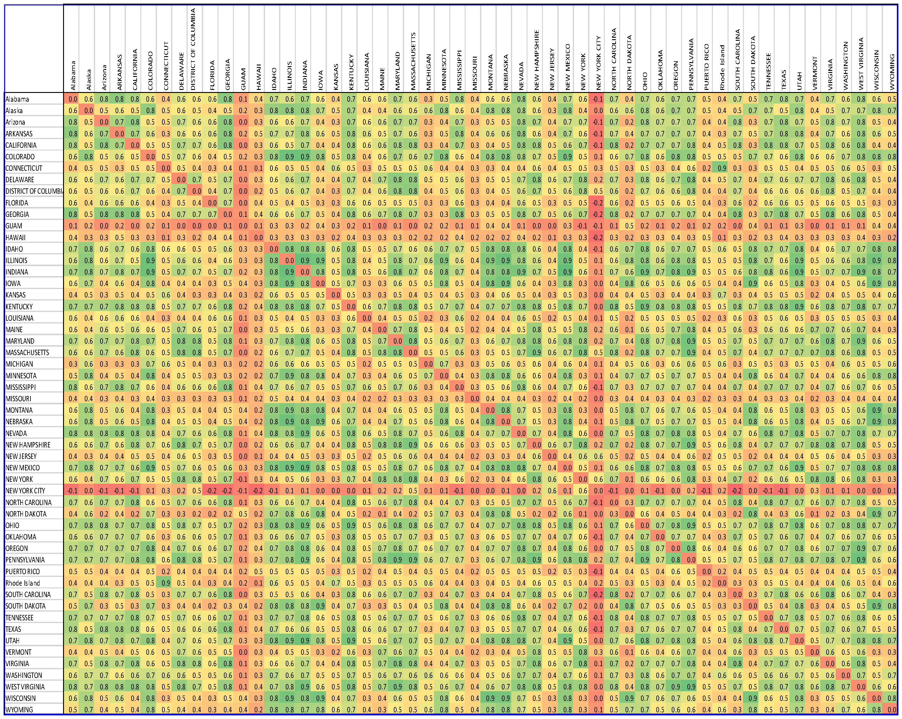
| Node ID | State | Degree Centrality |
|---|---|---|
| 1 | Alabama | 18 |
| 2 | Alaska | 18 |
| 3 | Arizona | 17 |
| 4 | Arkansas | 14 |
| 5 | California | 22 |
| 6 | Colorado | 20 |
| 7 | Connecticut | 1 |
| 8 | Delaware | 14 |
| 9 | District Of Columbia | 8 |
| 10 | Florida | 0 |
| 11 | Georgia | 18 |
| 12 | Guam | 0 |
| 13 | Hawaii | 0 |
| 14 | Idaho | 21 |
| 15 | Illinois | 22 |
| 16 | Indiana | 29 |
| 17 | Iowa | 14 |
| 18 | Kansas | 0 |
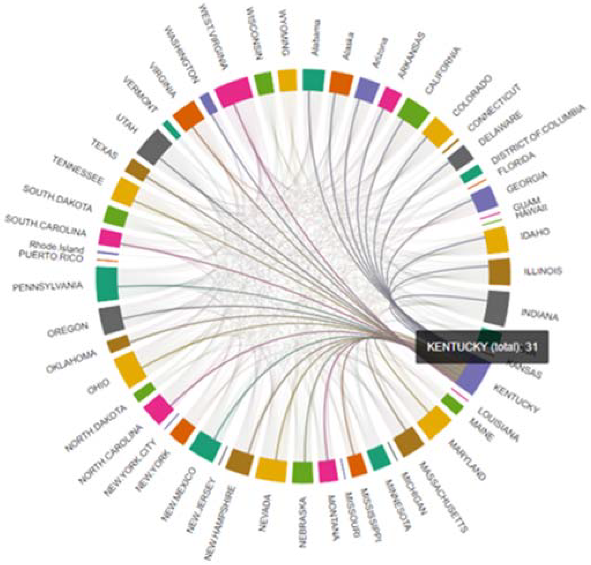
| 19 | Kentucky | 31 |
| 20 | Louisiana | 0 |
| 21 | Maine | 9 |
| 22 | Maryland | 24 |
| 23 | Massachusetts | 20 |
| 24 | Michigan | 0 |
| 25 | Minnesota | 15 |
| 26 | Mississippi | 13 |
| 27 | Missouri | 0 |
| 28 | Montana | 15 |
| 29 | Nebraska | 17 |
| 30 | Nevada | 25 |
| 31 | New Hampshire | 20 |
| 32 | New Jersey | 0 |
| 33 | New Mexico | 22 |
| 34 | New York | 14 |
| 35 | New York City | 0 |
| 36 | North Carolina | 19 |
| 37 | North Dakota | 8 |
| 38 | Ohio | 27 |
| 39 | Oklahoma | 10 |
| 40 | Oregon | 22 |
| 41 | Pennsylvania | 29 |
| 42 | Puerto Rico | 0 |
| 43 | Rhode Island | 1 |
| 44 | South Carolina | 13 |
| 45 | South Dakota | 14 |
| 46 | Tennessee | 20 |
| 47 | Texas | 12 |
| 48 | Utah | 26 |
| 49 | Vermont | 5 |
| 50 | Virginia | 21 |
| 51 | Washington | 8 |
| 52 | West Virginia | 29 |
| 53 | Wisconsin | 14 |
| 54 | Wyoming | 15 |
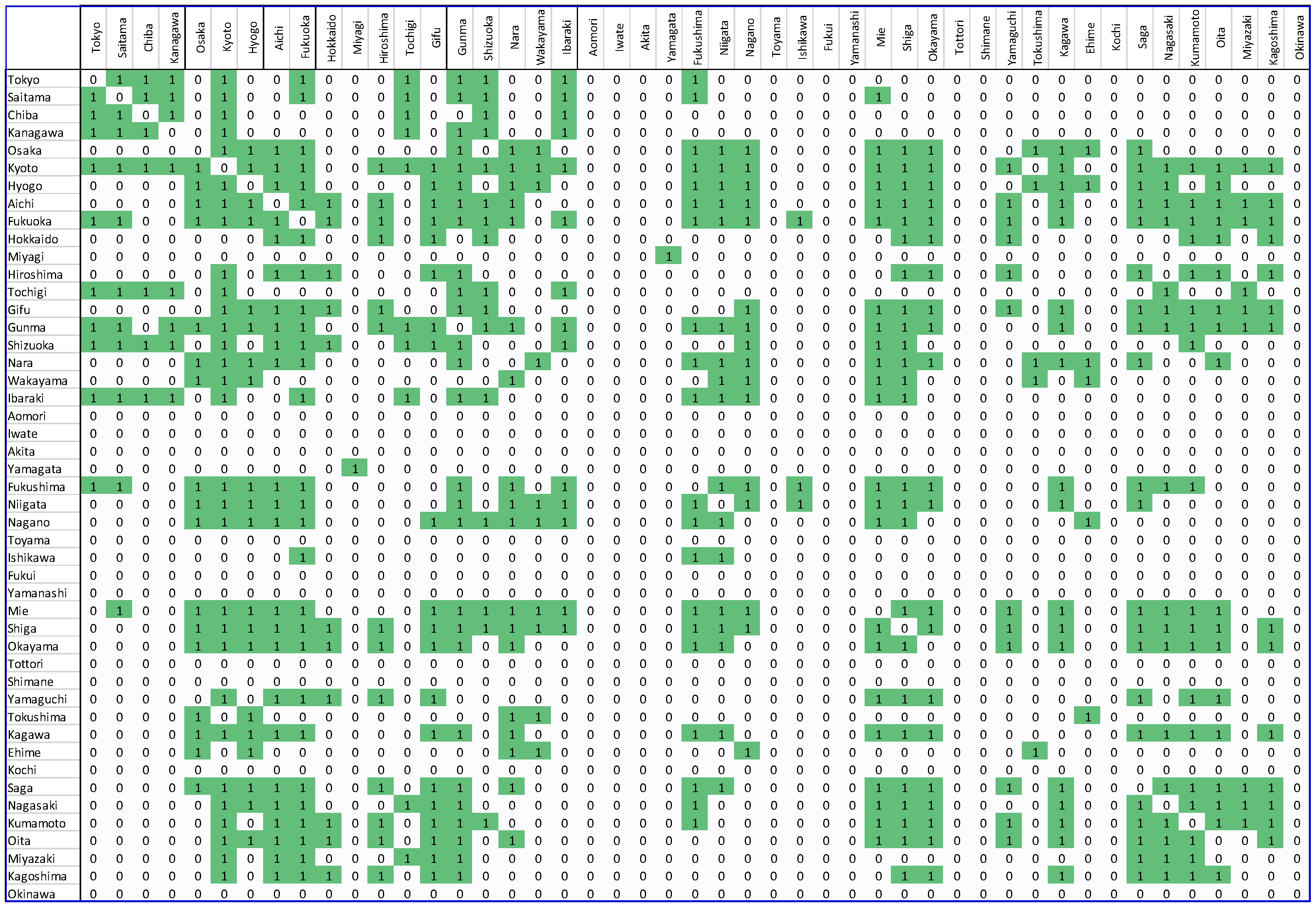
| Node ID | Prefectures | Degree Centrality |
|---|---|---|
| 1 | Tokyo | 10 |
| 2 | Saitama | 11 |
| 3 | Chiba | 7 |
| 4 | Kanagawa | 8 |
| 5 | Osaka | 17 |
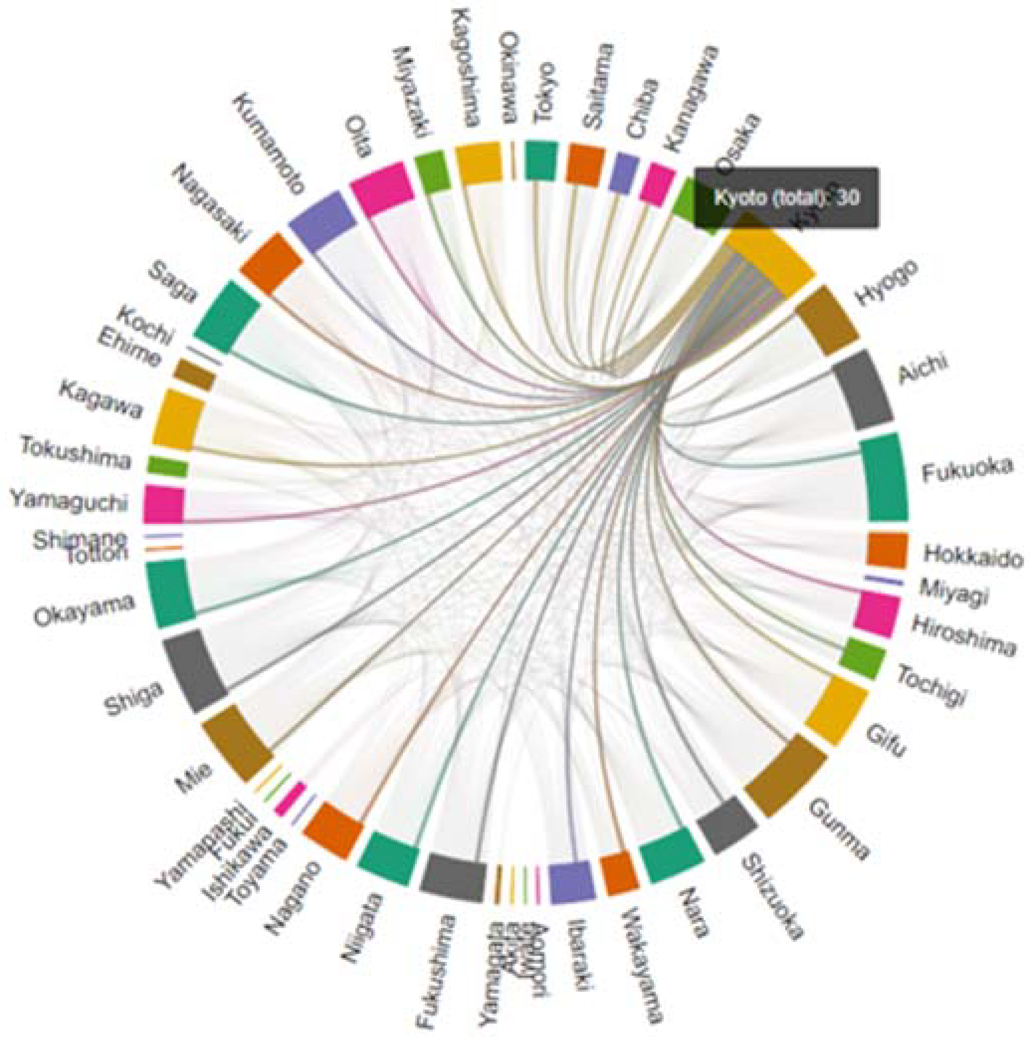
| 6 | Kyoto | 30 |
| 7 | Hyogo | 20 |
| 8 | Aichi | 24 |
| 9 | Fukuoka | 28 |
| 10 | Hokkaido | 11 |
| 11 | Miyagi | 1 |
| 12 | Hiroshima | 13 |
| 13 | Tochigi | 10 |
| 14 | Gifu | 20 |
| 15 | Gunma | 27 |
| 16 | Shizuoka | 16 |
| 17 | Nara | 18 |
| 18 | Wakayama | 10 |
| 19 | Ibaraki | 14 |
| 20 | Aomori | 0 |
| 21 | Iwate | 0 |
| 22 | Akita | 0 |
| 23 | Yamagata | 1 |
| 24 | Fukushima | 20 |
| 25 | Niigata | 17 |
| 26 | Nagano | 16 |
| 27 | Toyama | 0 |
| 28 | Ishikawa | 3 |
| 29 | Fukui | 0 |
| 30 | Yamanashi | 0 |
| 31 | Mie | 23 |
| 32 | Shiga | 25 |
| 33 | Okayama | 21 |
| 34 | Tottori | 0 |
| 35 | Shimane | 0 |
| 36 | Yamaguchi | 12 |
| 37 | Tokushima | 5 |
| 38 | Kagawa | 18 |
| 39 | Ehime | 6 |
| 40 | Kochi | 0 |
| 41 | Saga | 21 |
| 42 | Nagasaki | 17 |
| 43 | Kumamoto | 19 |
| 44 | Oita | 18 |
| 45 | Miyazaki | 9 |
| 46 | Kagoshima | 14 |
| 47 | Okinawa | 0 |
Publisher’s Note: MDPI stays neutral with regard to jurisdictional claims in published maps and institutional affiliations. |
© 2022 by the authors. Licensee MDPI, Basel, Switzerland. This article is an open access article distributed under the terms and conditions of the Creative Commons Attribution (CC BY) license (https://creativecommons.org/licenses/by/4.0/).
Share and Cite
Davahli, M.R.; Karwowski, W.; Fiok, K.; Murata, A.; Sapkota, N.; Farahani, F.V.; Al-Juaid, A.; Marek, T.; Taiar, R. The COVID-19 Infection Diffusion in the US and Japan: A Graph-Theoretical Approach. Biology 2022, 11, 125. https://doi.org/10.3390/biology11010125
Davahli MR, Karwowski W, Fiok K, Murata A, Sapkota N, Farahani FV, Al-Juaid A, Marek T, Taiar R. The COVID-19 Infection Diffusion in the US and Japan: A Graph-Theoretical Approach. Biology. 2022; 11(1):125. https://doi.org/10.3390/biology11010125
Chicago/Turabian StyleDavahli, Mohammad Reza, Waldemar Karwowski, Krzysztof Fiok, Atsuo Murata, Nabin Sapkota, Farzad V. Farahani, Awad Al-Juaid, Tadeusz Marek, and Redha Taiar. 2022. "The COVID-19 Infection Diffusion in the US and Japan: A Graph-Theoretical Approach" Biology 11, no. 1: 125. https://doi.org/10.3390/biology11010125
APA StyleDavahli, M. R., Karwowski, W., Fiok, K., Murata, A., Sapkota, N., Farahani, F. V., Al-Juaid, A., Marek, T., & Taiar, R. (2022). The COVID-19 Infection Diffusion in the US and Japan: A Graph-Theoretical Approach. Biology, 11(1), 125. https://doi.org/10.3390/biology11010125