Article

Modeling the Influence of Knots on Douglas-Fir Veneer Fiber Orientation

Arts et Metiers Institute of Technology, LaBoMaP, HESAM Université, 71250 Cluny, France
*
Author to whom correspondence should be addressed.
Fibers 2020, 8(9), 54; https://doi.org/10.3390/fib8090054
Submission received: 21 July 2020 / Revised: 6 August 2020 / Accepted: 18 August 2020 / Published: 21 August 2020

Abstract

:
This study presents a method for predicting the local fiber orientation of veneers made from peeled Douglas-fir logs based on the knowledge of the tree branch characteristics (location, radius, insertion angle, azimuth angle, and living branch ratio). This model is based on the Rankine oval theory approach and focuses on the local deviation of the fiber orientation in the vicinity of knots. The local fiber orientation was measured online during the peeling process with an in-house-developed scanner based on the tracheid effect. Two logs from the same tree were peeled, and their ribbons were scanned. The knot locations and fiber orientation were deduced from the scanner data. The first objective was to compare the fiber orientation model with measurements to enhance and validate the model for French Douglas-fir. The second objective was to link data measurable on logs to veneer quality.

1. Introduction

The majority of French Douglas-fir forests were planted in the period between the 1950s and the 1970s [1]. According to Thivolle-Cazat et al. [2], in the near future, a fraction of these forests will contain logs with diameters larger than 50 cm, which are rejected by industrial sawmills with the standard chipper canter. To transform these mature but often knotty trees, the peeling industry seems to be a sustainable option since large logs are not difficult to peel and the yield increases with the log diameter. However, the growing conditions of these trees can favor large knots; thus, veneers might present high fiber orientation deviation over a large area. These veneers are not suitable for classic plywood industries, which require a high proportion of high-quality veneers to build panels. Laminated veneer lumber (LVL) panels, in which veneers are glued mostly in the longitudinal direction, seem to be an adequate way to use these veneers, since, in this material, homogenization of the overall product is standard (facilitating better properties than solid wood [3,4,5,6]). Moreover, it is possible to improve the mechanical properties and natural durability of the product by sorting the veneers before LVL panel construction [7,8,9,10,11]. A method proposed by Bleron et al. [12] based on the local density can predict the mechanical properties of Douglas-fir products. This approach, despite promising results, requires an X-ray scan of each veneer.
This paper proposes a method for describing the knottiness based on data measurable from logs and the comparison and enhancement of a fiber deviation model in the vicinity of knots with online measurement of the fiber orientation. Firstly, the knot pattern is obtained using the peeling thickness, branch shape, and distribution along the log by virtually following the knife path during rotary cutting in accordance with Mothe et al. [13]. Then, the description of the fiber directions in the vicinity of the knots is computed from a mathematical formulation based on the Rankine oval [14]. This so-called flow-grain analogy was first described by Goodman and Bodig [15] and afterward by References [14,16,17]. Each knot is considered an elliptical obstacle to a constant flow.
A new apparatus (LOOBAR: local online orientation fiber analyzer) was designed to measure the local fiber orientation online to validate this approach. The fiber orientation measurement is based on the “tracheid effect” [18,19,20,21,22,23,24,25]. This device is described below. This technology is cheaper and simpler to install on a peeling line than X-ray peeling.
Viguier et al. [10] describes an innovative method based on the fiber local orientation to sort veneer and predict mechanical properties of beech laminated veneer lumber. The fiber orientation model, which is detailed in this paper, can be coupled with Viguier’s mechanical model to predict the mechanical potential of a forest or to sort veneers without another system of mechanical grading, in an industrial process.

2. Materials and Methods

2.1. Experimental Campaign

2.1.1. Log Sampling and Description

For this study, two logs were sawn from the same 29-year-old tree and selected for their proportion of living branches. The two logs were slightly conical (near 0.4°), and their average radial growth ring width was 5.7 mm. The first log measured 790 mm in length, and the two extremum circles had diameters of 340 mm for the base and 330 mm for the top. The second log measured 790 mm in length. The mean diameter of the base and that of the top were 350 mm and 340 mm, respectively.

2.1.2. Peeling Process

The peeling line used for this study was composed of an instrumented peeling machine (see Figure 1), a clipper, and a specifically designed laser scanner (LOOBAR). The logs were peeled at a set thickness of 3 mm close to the veneer standards for LVL production. The peeling speed was constant and set to 1.5 m·s−1. The veneers were clipped at a width of 750 mm perpendicular to the grain direction and almost equal to the log length.

2.1.3. Veneer Fiber Orientation Measurement

The LOOBAR is an experimental device based on the tracheid effect. The tracheid effect occurs when a laser pointer lights up a wood surface. The laser dot is distorted along the fiber direction (a circle becomes an ellipse under this effect). The scanner is composed of 50 5-mW laser pointers that are equally distributed over an 800-mm range along the principal fiber direction (see Figure 2) and four cameras (Basler acA2440-75 µm) with a resolution of 2048 × 120 pixels. The camera acquisition speed is as high as 1000 frames per second for this resolution, corresponding to a resolution of 3 mm perpendicular to the fiber direction for a cutting speed of 1.5 m·s−1. The resolution in the fiber direction is equal to the distance between two laser dots, which is nearly constant and close to 16 mm. All the laser pointers were independently calibrated to restitute a radiant flux of 1 mW using a photodiode sensor (Thorlab PM16-151).
The images taken by cameras are stitched and then binarized to detect the ellipses created by the laser pointers. The ellipse center location and major and minor axes are estimated with the library OpenCv [26] and the “FitEllipse” function. A similar method was used by References [10,27,28], yielding satisfying results.
After peeling, all the veneer color pictures are acquired by a cellphone camera (LG Nexus 5X -12.3 megapixels) and are used for the extraction of the exact position and radius of each knot along the ribbon. All the pictures are transformed with the library OpenCv [26] and the “findHomography” and “warpPerspective” functions. The knots are manually identified on color pictures. As the average branch insertion angle nears 80° (see Table 1 and Table 2), knots are considered circles. The shapes of the branches are close to circular, and the peeling logs are centered on the pith. Fitting the knots with a circle for the cutting mode (0–90°) [29] is an acceptable approximation.
Figure 3 presents the fiber orientation map superimposed on the color pictures of the first log ribbon. The fiber deviation area is clearly visible in the vicinity of the knots.

2.2. Modeling

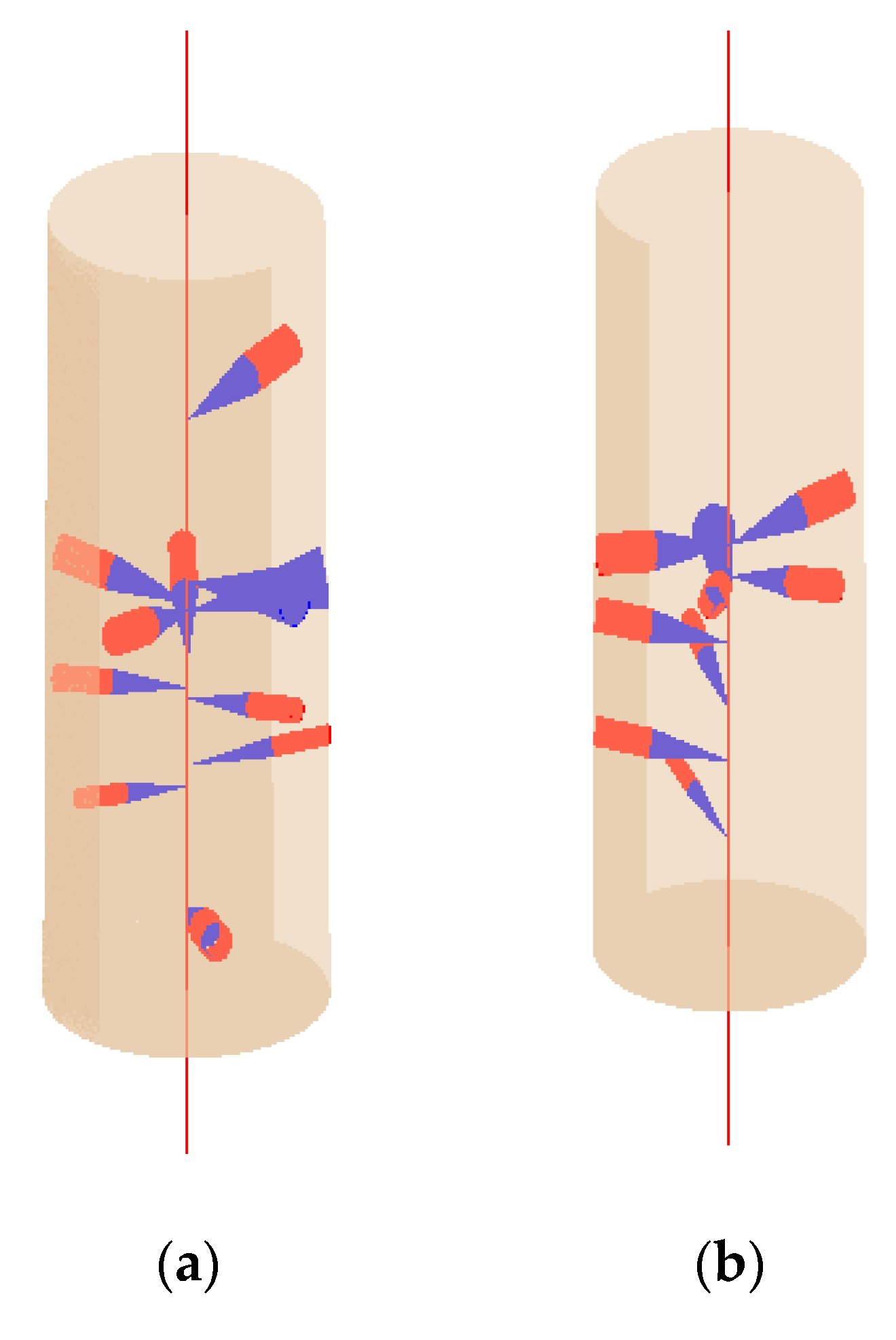
2.2.1. Log Description, Knot Location, and Radius

According to Mothe et al. [13], the branches into a log can be defined by five criteria (Figure 4). These criteria for each branch are the azimuth angle, the insertion angle, the location along the log, the living branch ratio, and the external diameter (close to the bark). According to the author, these parameters can be used to model the inner shape of the branches in a softwood log.
The azimuth and insertion angles were measured with a protractor. A plumb line was used to obtain the reference axis of the azimuth angle. The location along the log and the outer-log diameter were measured with a meter and a caliper. Hein et al. [30] modeled Douglas-fir branch characteristics; in accordance with the author’s model, if the branches were cut too close to the bark, the insertion angle was considered unmeasurable and was set to 80°. A living branch is defined as a cone (in blue) from the pith to the periphery of the log. A dead branch is defined by two parts: a cone (in blue) up to the death of the branch and a cylinder (in red) beyond (Figure 4), as the branch no longer has secondary growth. The living branch ratio (Equation (1)) is set to 1 for the living branches and 0.6 for the dead branches concordant with the Hein et al. [30] model.
Living   branch   ratio = ( Living   part   length Living + Dead   part   length ) .
The first log had 11 visible branches on its bark at the locations described in Table 1. This log contained a whorl between 450 mm and 400 mm from the base. The second log had nine visible branches on its bark at the locations described in Table 2. This log contained a crown of branches between 450 mm and 350 mm from the base.
Each log (see Figure 5) was defined by two extremity circles (top and bottom). A three-dimensional (3D) model was built using Python language with the library OpenGl [31]. Figure 5a,b shows visual representations of Log 1 and Log 2, respectively, according to the hypothesis made and the data presented in Table 1 and Table 2.
Both log models were virtually peeled to determine the knot locations on the ribbon by considering that the cutting knife follows an Archimedean spiral with a 3-mm peeling thickness path. The knot location was determined by the intersection between the knife cutting edge and the knots. Finally, the ribbon was clipped in 750-mm-wide veneers (see Figure 6).

2.2.2. Log Description, Knot Location, and Radius

The model proposed by Foley [14] was used to predict the local fiber orientation around the knots. The model is based on the Rankine oval method. A source and a sink with an equal flow rate are located in a constant flow to create a stagnation streamline. The freestream speed is fixed (see Figure 7) to determine the flow of the source and the sink. The stagnation point and stagnation streamline are computed to find the source and the sink flows and their distances from the oval center. The model parameters that are fixed to determine the oval are b r 2 , the half-height of the knot, L r 2 , the half-width, and U , the freestream speed. The height of the knot is equal to its width in our case since the knots are considered circles. A numerical minimization of the function f a , m (Equation (2)) must be computed according to Foley [14] to determine the parameters m and a, which are the source and sink strength and the half-distance between the source and the sink, respectively. This method was detailed in References [14,17,32,33].
f a , m = ( cot ( b r / 2 a 2 × m U × a ) b r / 2 a ) 2 + ( 1 + 2 × m U × a L r / 2 a ) 2 .
The velocity vector around the knots is computed, and its direction gives the fiber orientation. The veneer fiber orientation (combination of multiple knots) is obtained by linearly adding the main flow, sink flow, and source flow obtained for each knot (Figure 8).

3. Results and Discussion

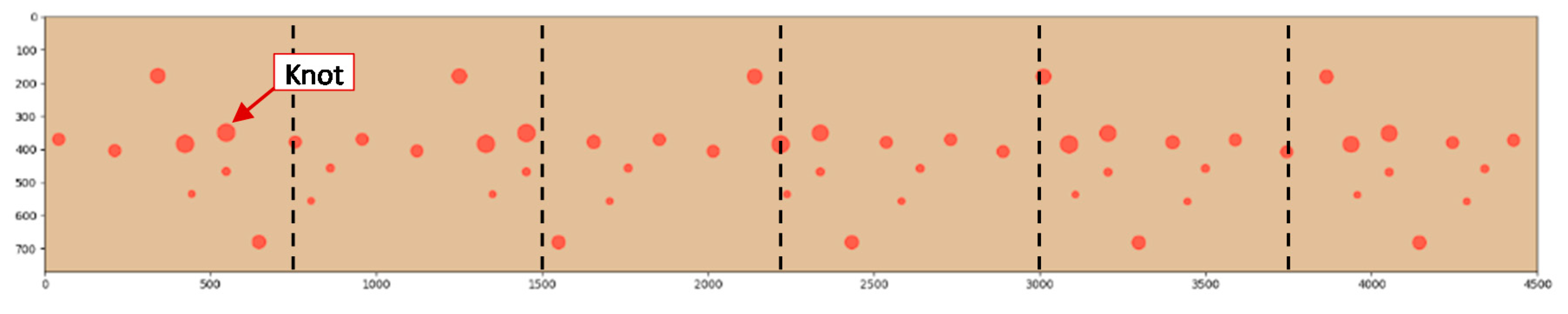
3.1. Knot Location and Radius

The modeled knot center and radius were compared to those obtained from the pictures taken by cellphone. Figure 9a,b presents the real knots in red and the predicted knots in green, superimposed on the color pictures, for the three first veneers and the three last veneers of both log ribbons. The knot location error that appeared for the core veneers (Figure 9a,b) could be due to miscentering during the peeling process or inaccuracy in the branch measurement. The model of the knot (cone-cylinder) can also affect the radius estimation. Only the knots visible before peeling can be located. Consequently, branches hidden before peeling cannot be modeled. For the veneers peeled from the two logs, 369 knots were predicted from a total of 537 knots, which represents 69% of the knots. However, the nonmodeled knots were principally the smallest knots; 90% had radii smaller than 11 mm. The mean radius of the nonmodeled knots was 7.88 mm compared with 17.12 mm for the detected knots (Figure 9c).
The distances between the ellipse centers of the measured and predicted knots were compared (see Figure 9d). The median distance was 19.91 mm. The median of the relative error between the measured and modeled knot radii was near 0% (see Figure 9e). The hypothesis presented in Section 2.2.1 (0.6 live parts of branch) seems to be reliable. The relative error of the radius was between −25% and +25%, which shows that there was no large bias. Finally, a minor shift in the measured knot location did not have an important impact on the fiber orientation, in contrast to the number of predicted knots and their radius on the total length of the ribbon. Furthermore, the relative error of the radius was centered on zero, and an overestimated radius may be compensated for by an underestimated radius (symmetry of the distribution). Therefore, the model can be an interesting approximation for predicting knot characteristics to determine the mechanical properties of veneers.

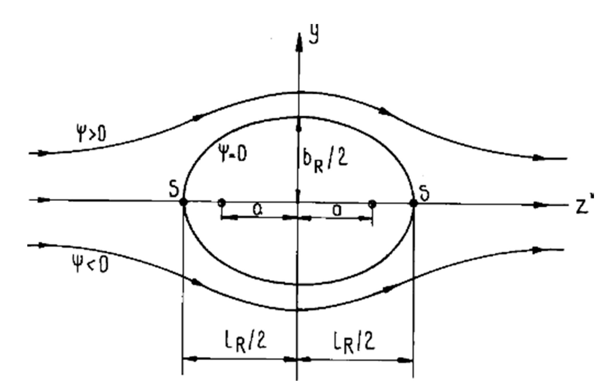
3.2. Fiber Orientation in the Vicinity of Knots

The fiber direction with the Rankine oval model was compared to the local fiber orientation, which was measured with LOOBAR. The Rankine oval model was applied using the diameter and center location of the measured knots to focus only on the performance of this approach.
A threshold was defined using the ratio between the major axis and the minor axis to ensure that the ellipses were correctly fitted over the observed laser patterns. For ratios lower than 1.45, the ellipses were not taken into account. Actually, when an ellipse is close to a circle (ratio close to 1), some error of fitting can occur because a circle has no observable major axis, in contrast to an ellipse. Additionally, only angles between −45° and 45° were taken into account to discard these kinds of outliers.
A qualitative validation was performed to ensure that the regions of interest around the knots were adequate with the hypothesis on the restricted angles and ratio. This was achieved by superimposing the knots detected manually (red circles) and the measured fiber orientation (arrows) on the color picture (see Figure 10a,b). Moreover, only the ellipse angles with a maximal distance from the knot center were taken into account in order to focus on the local impact of the knots. The standard deviation of all the ellipse angles contained in an annulus area with a size 0.1 radius was shifted from one to five radii to determine this maximal distance (Figure 10b,c). The distance to the knot center was normalized by the knot radius.
The knot radius range was selected to obtain a sufficient number of knots in each bin (Table 3). The precision of the standard deviation for the first bin (radii from 3 mm to 8 mm) was affected by the small number of measured ellipses with regard to the other bins.
The maximal distance of the perturbation area was fixed at a radius of 3.4 to the knot center, as the evolution seemed to reach an asymptote. This methodology ensures a focus on the fiber orientation deviation in a region close to the knot and excluding the knot itself.
An innovative way to present the results is proposed in Figure 11, expressing the robustness of this approach. The general purpose is to show the fiber orientation deviation for all the knots in one graph. Figure 11a presents the measured angles of all the knots, for a total of 289 knots and 40,137 measured angles, for all the veneers peeled from log 1. The fiber orientation around the knots seems to vary linearly on a knot radius basis. The perturbation area was proportional to the size of the knots (see Figure 10c). Therefore, small knots should have a mechanical impact on a relatively small zone.
The Foley (2003) model was used to predict the angles according to the approach detailed in Section 2.2.2. Figure 11b (the so-called base model) presents the raw modeled and normalized angles with the same knot radius as that for Figure 11a for the measured angles. The influence of the other knots in the vicinity can be observed on the left of Figure 11b.
The angles were linearly interpolated on a regular grid to determine the angles at every point, and streamlines were plotted to compare the measured and modeled angles (Figure 11d,e). The variation in the angle values expressed by the color scale shows that the values of the modeled angles were higher in the close vicinity of knots than those of the measured angles for the both raw and interpolated angle maps. To improve the efficiency of the model, it is possible to optimize its parameters as described below.
According to Foley (2003), a pattern in the vicinity of a knot may be defined with two different shapes. The first shape is derived from the Rankin oval pattern for representing the orientation of the fibers of the wood tissue connected to the branch. The second shape represents the orientation the fiber of the wood that passes around the knots. In our case, the pattern around the knots was not truly known. Therefore, the pattern of the fiber orientation can be modified using the six factors described by Foley (2003), which are listed in Table 4. An optimization of these adjustment factors was computed for log 1 to improve the model of the fiber orientation. The root-mean-square errors (RMSEs) were computed to find the best fit using an evolutionary algorithm (Bäck et al. 2018) to determine the best adjustment of the factors (Table 4). Figure 11c,f presents the enhanced model raw data and interpolated data to verify whether the measured streamline matched the enhanced modeled streamline. In fact, the perturbation area seemed larger for the measured raw data; however, after the interpolation, the enhanced model seemed to match the measurement results. Many points can be superimposed on the raw data figure, and they can mask each other. Therefore, interpolated data with streamlines are a better representation for comparing the model and measurements.
The best computed root-mean-square error (RMSE) was 8.70° on all the measured angles at a 3.4 knot–radius maximum distance. A control of these optimized factors was assessed for log 2. The optimized factors were applied to compute the angle RMSE for log 2. The result is satisfying since 9.57° is close to the RMSE obtained for the calibration step.
The fiber orientation enhanced model is based on the accurate measurement of the fiber orientation with the tracheid effect.
The addition of the characteristic of the fiber angle in the vicinity of knots is an interesting way to improve the prediction of the mechanical properties of veneers. Finally, as the way the fibers deviate around a knot is proportional to the size of the knot, the size and location of knots can be sufficient to estimate the fiber orientation map of veneers. Nevertheless, this case work is only for the peeling process when the log is centered and the branch insertion angles are nearly normal from the pith of log, which yields circular knots.

4. Conclusions

It is possible to predict the fiber direction of peeled veneers from a log with branch characteristics. The knot size and location can be predicted on a veneer with no large biases. The fiber direction measured using a new experimental apparatus (LOOBAR) was compared to the direction predicted using the Rankine oval model. The Rankine oval model was adjusted to approximate the measured fiber direction. Finally, the information given by the size of knots can be sufficient because the pattern around the knots seems to be proportional to their size. This observation can be very useful for developing a simple model of local orientation fiber deviation based on a function proportional to the knot radius. A supplementary interest is the simplification of the fiber orientation measurement system by knot detection with scatter, which is easily transferable industrially.
Of course, this approach needs a larger amount of data to be fully validated. Different types of logs have to be tested regarding their proportion of living branches and silvicultural–scenario effects.
Nevertheless, the general method can be used to predict the mechanical properties of engineering wood material such as plywood or laminated veneer lumber. However, other information, such as the ring width, needs to be taken into account to evaluate the mechanical properties of a given resource. Therefore, it is possible to grade veneers before or during the peeling process to optimize the final products with only knowledge of the branch characteristics.

Author Contributions

Conceptualization, R.F., S.G., L.D., and R.C.; methodology, R.F. and S.G.; software, R.F.; validation, R.F., S.G., L.D., and R.C.; formal analysis, R.F.; investigation, R.F.; resources, R.F. and R.C.; data curation, R.F.; writing—original draft preparation, R.F.; writing—review and editing, R.F., S.G., L.D., and R.C.; visualization, R.F.; supervision, R.C., S.G., and L.D.; project administration, R.F., S.G., L.D., and R.C.; funding acquisition, R.C. All authors have read and agreed to the published version of the manuscript.

Funding

This work was conducted thanks to the support of the Région Bourgogne Franche-Comté, the Ministère de l’Alimentation et de l’Agriculture Francais, and the Xylomat Technical Platform from the Xylomat Scientific Network funded by ANR-10-EQPX-16 XYLOFOREST.

Acknowledgments

The authors would also like to thank Benjamin Roux, who developed the new scanner (LOOBAR), the Office National des Forêts (ONF), and the Institut National de la Recherche Agronomique (INRA).

Conflicts of Interest

The authors declare no conflict of interest.

References

  1. Claire, R. Le Douglas un Arbre Exceptionnel; Imprimerie Scheuer: Drulingen, UK, 2010; ISBN 2-913162-94-0. [Google Scholar]
  2. Thivolle-Cazat, A.; Weiller, G.; Bailly, A. Ressource et Disponibilité en Douglas en France. In Proceedings of the Assises nationales du douglas, Bordeaux, France, 19–21 September 2018. [Google Scholar]
  3. Collet, R.; Bleron, L. Perspectives de valorisation et de transformation du douglas en Bourgogne; Forêt Entreprise n°188: Paris, France, 2009; pp. 27–31. [Google Scholar]
  4. Ebihara, T. The performance of composite beams with laminated-veneer lumber (LVL) flanges. J. Jpn. Wood Res. Soc. 1982, 28, 216. [Google Scholar]
  5. Eckelman, C. Potential uses of laminated veneer lumber in furniture. For. Prod. J. 1993, 43, 19. [Google Scholar]
  6. Youngquist, J.; Laufenberg, T.; Bryant, B.S. End jointing of laminated veneer lumber for structural use. For. Prod. J. 1984, 34, 25–32. [Google Scholar]
  7. Del Menezzi, C.; Mendes, L.; de Souza, M.; Bortoletto, G. Effect of Nondestructive Evaluation of Veneers on the Properties of Laminated Veneer Lumber (LVL) from a Tropical Species. Forests 2013, 4, 270–278. [Google Scholar] [CrossRef] [Green Version]
  8. Pu, J.; Tang, R.C. Nondestructive evaluation of modulus of elasticity of southern pine lvl: Effect of veneer grade and relative humidity. Wood Sci. Technol. 1997, 29, 249–263. [Google Scholar]
  9. De Souza, F.; Del Menezzi, C.; Júnior, G.B. Material properties and nondestructive evaluation of laminated veneer lumber (LVL) made from Pinus oocarpa and P. kesiya. Eur. J. Wood Wood Prod. 2011, 69, 183–192. [Google Scholar] [CrossRef]
  10. Viguier, J.; Bourgeay, C.; Rohumaa, A.; Pot, G.; Denaud, L. An innovative method based on grain angle measurement to sort veneer and predict mechanical properties of beech laminated veneer lumber. Constr. Build. Mater. 2018, 181, 146–155. [Google Scholar] [CrossRef]
  11. Wang, X.; Ross, R.J.; Brashaw, B.K.; Verhey, S.A.; Forsman, J.W.; Erickson, J.R. Flexural Properties of Laminated Veneer Lumber Manufactured from Ultrasonically Rated Red Maple Veneer: A Pilot Study; U.S. Department of Agriculture, Forest Service, Forest Products Laboratory: Madison, WI, USA, 2003. [Google Scholar]
  12. Bleron, L.; Collet, R.; Marchal, R.; Mothe, F.; Nepveu, G. Methods of Simulation Allowing the Characterization of Veneer Products Resulting from the Transformation of Douglas-fir. In Proceedings of the Second International Symposium Veneer Processing and Products (ISVPP2), Vancouver, BC, Canada, 9–10 May 2006; pp. 321–328. [Google Scholar]
  13. Mothe, F.; Thibaut, B.; Marchal, R.; Negri, M. Rotary Cutting Simulation of Heterogeneous Wood: Application to Douglas for Peeling. Available online: http://agritrop.cirad.fr/391663/ (accessed on 27 November 2017).
  14. Foley, C. Modeling the Effects of Knots in Structural Timber; División of the Structural Engineering, Lund University: Lund, Sweden, 2003. [Google Scholar]
  15. Goodman, J.R.; Bodig, J. Mathematical model of the tension behavior of wood with knots and cross grain. In Proceedings of the First International Conference on Wood Fracture, Banff, AB, Canada, 14–16 August 1978. [Google Scholar]
  16. Kandler, G.; Lukacevic, M.; Füssl, J. An algorithm for the geometric reconstruction of knots within timber boards based on fibre angle measurements. Constr. Build. Mater. 2016, 124, 945–960. [Google Scholar] [CrossRef]
  17. Lukacevic, M.; Kandler, G.; Hu, M.; Olsson, A.; Füssl, J. A 3D model for knots and related fiber deviations in sawn timber for prediction of mechanical properties of boards. Mater. Des. 2019, 166, 107617. [Google Scholar] [CrossRef]
  18. Belkacemi, M.; Massich, J.; Lemaitre, G.; Stolz, C.; Daval, V.; Pot, G.; Aubreton, O.; Collet, R.; Meriaudeau, F. Wood Fiber Orientation Assessment Based on Punctual Laser Beam Excitation: A Preliminary Study; QIRT Council: Gdansk, Poland, 2016. [Google Scholar]
  19. Briggert, A.; Hu, M.; Olsson, A.; Oscarsson, J. Tracheid effect scanning and evaluation of in-plane and out-of-plane fiber direction in norway spruce timber. Wood Fiber Sci. 2018, 50, 411–429. [Google Scholar] [CrossRef] [Green Version]
  20. Daval, V.; Pot, G.; Belkacemi, M.; Meriaudeau, F.; Collet, R. Automatic measurement of wood fiber orientation and knot detection using an optical system based on heating conduction. Opt. Express 2015, 23, 33529–33539. [Google Scholar] [CrossRef] [PubMed] [Green Version]
  21. Faydi, Y.; Viguier, J.; Pot, G.; Daval, V.; Collet, R.; Bléron, L.; Brancheriau, L. Modélisation des propriétés mécaniques du bois à partir de la mesure de la pente de fil. In Proceedings of the 22ème Congrès Français de Mécanique, Lyon, France, 24–28 August 2015. [Google Scholar]
  22. Hu, C.; Tanaka, C.; Ohtani, T. On-line determination of the grain angle using ellipse analysis of the laser light scattering pattern image. J. Wood Sci 2004, 50, 321–326. [Google Scholar] [CrossRef]
  23. Nyström, J. Automatic measurement of fiber orientation in softwoods by using the tracheid effect. Comput. Electron. Agric. 2003, 41, 91–99. [Google Scholar] [CrossRef]
  24. Simonaho, S.-P.; Palviainen, J.; Tolonen, Y.; Silvennoinen, R. Determination of wood grain direction from laser light scattering pattern. Opt. Lasers Eng. 2004, 41, 95–103. [Google Scholar] [CrossRef]
  25. Zhou, J.; Shen, J. Ellipse detection and phase demodulation for wood grain orientation measurement based on the tracheid effect. Opt. Lasers Eng. 2003, 39, 73–89. [Google Scholar] [CrossRef]
  26. OpenCV Team. OpenCV; OpenCV Team: San Francisco, CA, USA, 2019. [Google Scholar]
  27. Olsson, A.; Pot, G.; Viguier, J.; Faydi, Y.; Oscarsson, J. Performance of strength grading methods based on fibre orientation and axial resonance frequency applied to Norway spruce (Picea abies L.), Douglas fir (Pseudotsuga menziesii (Mirb.) Franco) and European oak (Quercus petraea (Matt.) Liebl/Quercus robur L.). Ann. For. Sci. 2018, 75. [Google Scholar] [CrossRef] [Green Version]
  28. Purba, C.Y.C.; Viguier, J.; Denaud, L.; Marcon, B. Contactless moisture content measurement on green veneer based on laser light scattering patterns. Wood Sci. Technol. 2020. [Google Scholar] [CrossRef]
  29. McKenzie, W.M. Fundamental Analysis of The Wood-Cutting Process; University of Michigan: Ann Arb, MI, USA, 1961. [Google Scholar]
  30. Hein, S.; Weiskittel, A.R.; Kohnle, U. Models on Branch Characteristics of Wide-Spaced Douglas-fir. For. Growth Timber Qual. Crown Models Simul. Methods Sustain. For. Manag. 2009, 12, 23. [Google Scholar]
  31. Kronos Group. OpenGL; Kronos Group: Beaverton, OR, USA, 2019. [Google Scholar]
  32. Foley, C. A three-dimensional paradigm of fiber orientation in timber. Wood Sci. Technol. 2001, 35, 453–465. [Google Scholar] [CrossRef]
  33. Phillips, G.; Bodig, J.; Goodman, J. Flow-grain analogy [Physical properties of coniferous wood]. Text. Chem. Colorist 1981, 14, 55. [Google Scholar]
Figure 1. Experimental peeling line from LaBoMaP.
Fibers 08 00054 g001
Figure 2. Picture of the local online orientation fiber analyzer (LOOBAR) laser scanner.
Fibers 08 00054 g002
Figure 3. Fiber orientation (°) measured by the scanner and superimposed on the color picture for the first log ribbon.
Fibers 08 00054 g003
Figure 4. Schematic of selected branch criteria.
Fibers 08 00054 g004
Figure 5. (a) Visual representation of log 1; (b) visual representation of log 2.
Fibers 08 00054 g005
Figure 6. Example of veneer knot map.
Fibers 08 00054 g006
Figure 7. Rankine oval stream function around an elliptical object [14].
Fibers 08 00054 g007
Figure 8. Fiber deviation map (°).
Fibers 08 00054 g008
Figure 9. (a) Predicted knots in green and real knots in red for the first and last parts of the log 1 ribbon; (b) predicted knots in green and real knots in red for first and last parts of the log 2 ribbon; (c) knot radius histograms; (d) distance from predicted knot center to real knot center; (e) relative error of radius.
Fibers 08 00054 g009
Figure 10. (a) Fiber angle measured with the threshold around the knots; (b) magnification of a knot with an example of the annulus measurement area; (c) standard deviations of angles in annulus areas for different knot sizes (mm).
Fibers 08 00054 g010
Figure 11. Comparison of the measured angles, the base model angles, and the enhanced model angles (°). Raw data (a) measured, (b) computed with base model, (c) computed with enhanced model; Data interpolated on regular grid (d) measured, (e) computed with base model, (f) computed with enhanced model.
Fibers 08 00054 g011
Table 1. Measured information of the first log branches.
Location
(mm)
Diameter
(mm)
Insertion Angle
(°)
Azimuth
(°)
Living Branch Ratio
617.042.078.01010.6
444.760.680.51821.0
424.135.980.03440.6
410.261.682.01331.0
417.137.880.02640.6
393.634.971.0500.6
338.225.680.03060.6
328.325.580.01820.6
259.920.180.01410.6
238.820.580.02830.6
115.539.080.02210.6
Table 2. Measured information of the first log branches.
Location
(mm)
Diameter
(mm)
Insertion Angle
(°)
Azimuth
(°)
Living Branch Ratio
450.738.680.01900.6
429.541.087.0210.6
428.233.780.03150.6
418.433.280.02540.6
372.555.081.01201.0
347.535.080.0380.6
277.225.680.01100.6
225.030.080.0380.6
140.020.080.01010.6
Table 3. Measured information of the first log branches.
Knot Radius Range
(mm)
Number of Knots Number of Ellipses from 1 to 5 Radii
3 ≤ knot size < 8371311
8 ≤ knot size < 139617,026
13 ≤ knot size < 183311,934
18 ≤ knot size < 238447,859
23 ≤ knot size < 283737,119
Table 4. Adjustment factors for the Rankine oval for Douglas-fir.
Value
A f l o w , b e l o w 0.528
A f l o w , a b o v e 0.572
B f l o w , b e l o w 0.099
B f l o w , a b o v e 0.099
Y o r e l Y o j · l 31.53
Y o l i m 8.52

