Article

Kinetics of Thermally Activated Physical Processes in Disordered Media

by
Bertrand Poumellec
and
Matthieu Lancry
*
Institut de Chimie Moléculaire et des Matériaux d'Orsay, Université Paris Sud, UMR CNRS-UPSud 8182, Orsay Center, 91405 Orsay, France
*
Author to whom correspondence should be addressed.
Fibers 2015, 3(3), 206-252; https://doi.org/10.3390/fib3030206
Submission received: 7 January 2015 / Accepted: 1 April 2015 / Published: 15 July 2015

Abstract

:
We describe a framework for modeling the writing and erasure of thermally-distributed activated processes that we can specifically apply to UV-induced refractive index change, particularly in fibers. From experimental measurements (isochrons and/or isotherms), this framework allows to find the distribution function of the activation energy by providing only a constant, which can be determined by a simple variable change when a few assumptions are fulfilled. From this modeling, it is possible to know the complete evolution in time of the system. It is also possible to determine the annealing conditions for extending a lifetime. This approach can also be used for other physical quantities, such as photodarkening, stress relaxation, and luminescence decay, provided that it can be described by a distribution function.

1. Problem: Dynamic Evolution of Physical Quantities in Disordered Media

UV-written intracore Fiber Bragg gratings are now routinely used for applications in optical telecommunications or as sensors in civil engineering. Most applications require a long grating lifetime. For example, in dense wavelength-division multiplexing (DWDM) optical communication systems, the grating-based devices should continue working at an agreed specification for 25 years in the temperature range −40 °C < θ < 80 °C. Accordingly, several theoretical and/or experimental studies, dealing with accelerated lifetime tests, have been carried out with a view to forecast possible degradation of the UV-induced refractive index changes [1,2].
For modeling the relaxation processes in disordered media, several approaches can be used and an extended report can be found in the reference book of Richert and Blumen [3]. The main problem is to account for the effect of disorder on thermally activated processes. The disorder can have an impact on the various steps of the physico-chemical reaction, leading to a change in the observed quantity (e.g., index changes, radiation-induced losses, etc.). For instance, if hopping is concerned in the reaction, the disorder will appear in the hopping distance or in the waiting time, if an energy barrier is involved, the activation energy will be distributed because the transition and/or the stable state configurations are varied.
These two examples differ fundamentally on one point: the temperature will not affect, in the same way, the range limit or the temperature-activated hopping. In particular, the dependence on the stability of refractive index with the writing or the ageing temperature [4] can be only explained by processes with distributed activation energies. Other arguments connected to changes in the structure reinforce this conclusion. However, a process like decoration of defect networks with H will not necessarily be relevant to a thermally activated process. In this paper, we consider only processes involving the distribution of activation energies as it is seen that this approach yield good results [1,5,6] with regards to the problem of index stability.

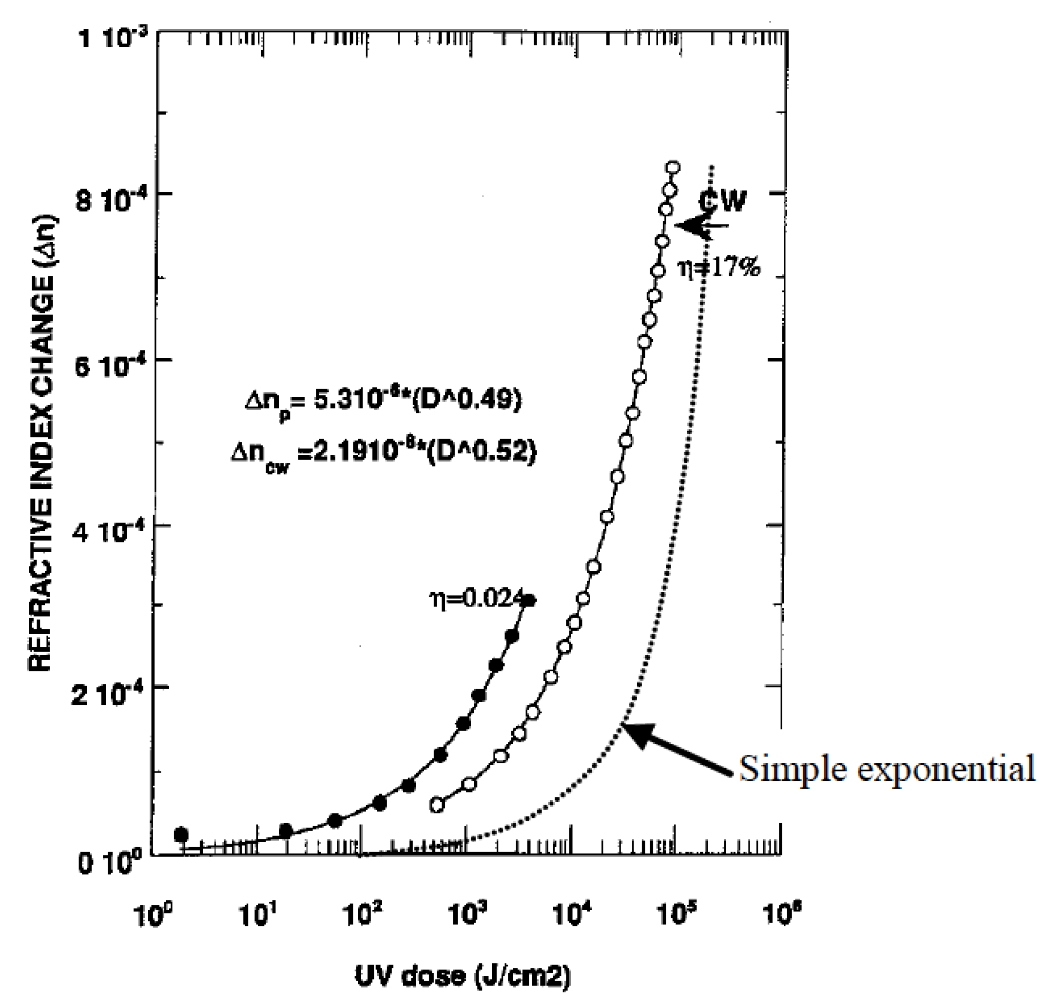
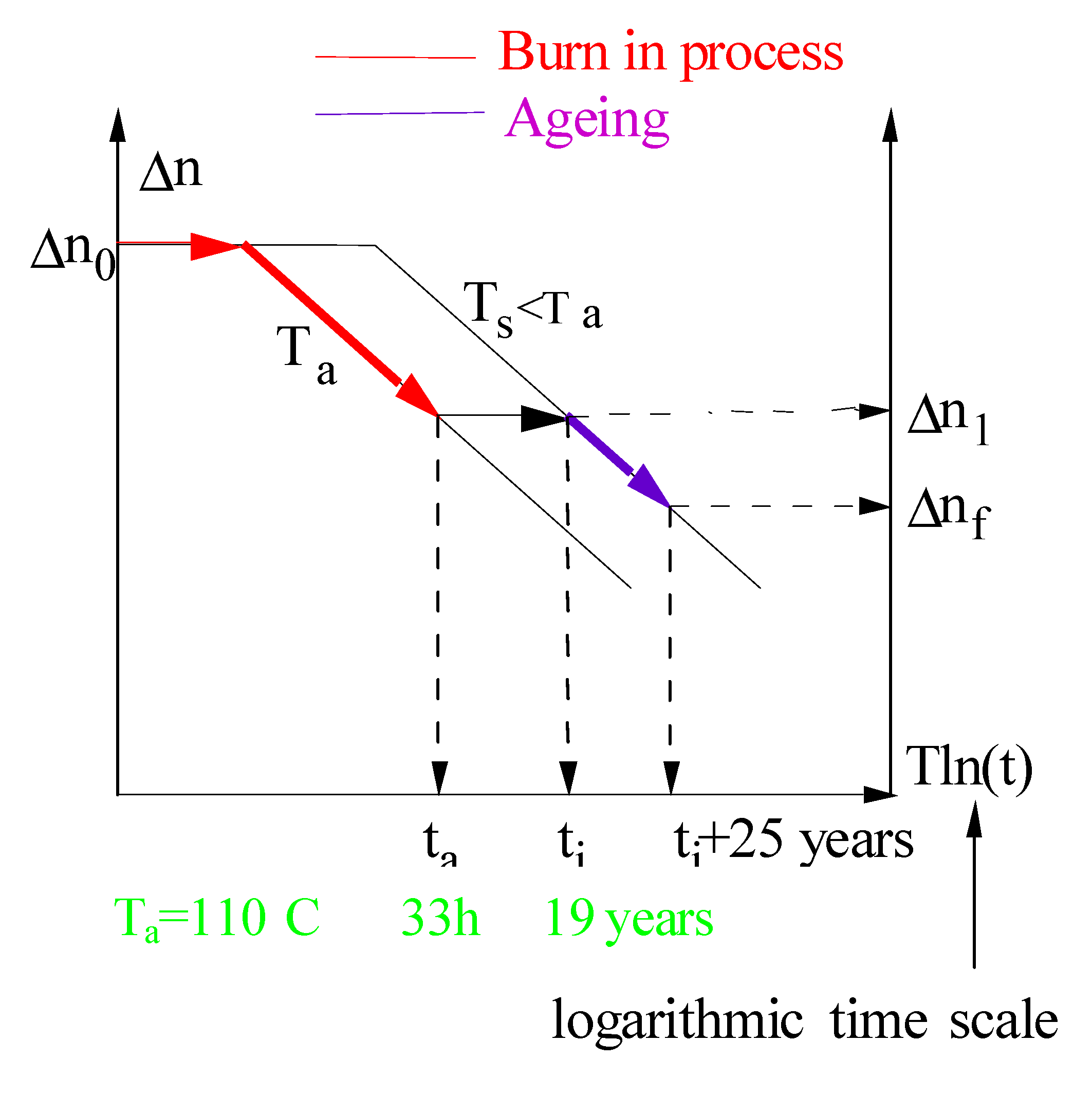
1.1. Under an External Action

Maybe the most important example of distributed processes for people working in the fabrication of telecommunication devices is the non-exponential growth of refractive index change under UV irradiation. In Figure 1 we can see that for a pulsed 248 nm laser, the index change grows according to a power law with an exponent of 0.5 [7]. In a number of fibers, this law is followed with an exponent between 0.25 and 0.8. We know from [8] that an index change in Ge-doped glasses is achieved by UV induced compaction. It is known that it is possible to achieve compaction in pure silica by the same means [9], but it is also possible to obtain compaction by ion or electron irradiation. Primak [10] is probably the author who studied these processes the most.
We can see in Figure 2 that compaction follows a power law again, with an exponent of 0.66. More recently, Allan et al. [11] showed that 193 nm irradiation in pure silica leads to densification by two-photon absorption (Figure 3).
We note in this case that the dose is no longer the relevant parameter but I2N, where I is the power density and N is the pulse number. The behavior is a power law with an exponent of 0.7.
Another example is the IR darkening of the Ge/Al/Er-codoped core optical fibers, observed under an H2 atmosphere of 0.012 atm, as shown in Figure 4 and Figure 5. Lemaire et al. [12] showed that OH vibration absorption at 1.38 μm also follows a power law in the same kind of experiment, the exponent of which increases linearly with temperature. Moreover, they have observed that the logarithm of the pre-exponential factor also evolves linearly with temperature. The power law is not the only behavior recorded in H2-induced IR darkening of fibers. Similar sensitivity of erbium-doped fibers to hydrogen has been reported in [13]. Rush et al. [14] showed that, in the case of phosphorus doped core optical fibers, a logt law leads to a better fit in a larger range of time (Figure 6). The same type of law has been invoked in transient creep experiments in metals. In this case, a constant distribution of sites is inferred [15].
Figure 1. Index change under UV irradiation, reprinted with permission from [7]. Copyright 1996 Elsevier.
Fibers 03 00206 g001
Figure 2. Electron irradiation induced compaction, reprinted with permission from [10]. Copyright 1968 AIP.
Fibers 03 00206 g002
Figure 3. Densification in fused silica under 193 nm irradiation, reprinted with permission from [11]. Copyright 1996 OSA. The optical path difference follows: O P D = a ( I 2 N ) 0.7 .
Fibers 03 00206 g003
Figure 4. IR darkening of the Ge-doped core optical fiber, reprinted with permission from [12]. Copyright 1991 SPIE. The OH growth data are well described by an equation of the form: Δ α OH = a ( t ) m , a = a 0 exp ( T / T 0 ) .
Fibers 03 00206 g004
Figure 5. a and m coefficients deduced from non-linear data fitting procedure.
Fibers 03 00206 g005
Last example for completing the panel of non-exponential behavior of systems submitted to an external action is the bleaching of the 400 nm luminescence by 266 nm light in Ge-doped core optical fibers (Figure 7). In that case, a stretched exponential law is used (exp(−αtβ)) and the exponent β is found depending linearly on power density [16]. Of course, this list is not exhaustive and is just made to show the spreading of the non-exponential behavior. It is valuable to see that non-exponential processes occur also spontaneously, without any external action.
Figure 6. IR Hydrogen induced darkening, reprinted with permission from [14]. Copyright 1983 IEEE.
Fibers 03 00206 g006
Figure 7. (a) Bleaching of 400 nm luminescence by 266 nm light in Ge-doped SiO2 fibers, reprinted with permission from [16]. Copyright 1993 OSA; (b) Exponent β of the stretched exponential law according to the power density.
Fibers 03 00206 g007

1.2. Thermal Relaxation

Of course, the most well known example in our field is the UV-induced refractive index change relaxation (Figure 8). The most popular law in this field is the inverse power law or sigmoidal law, studied by Erdogan et al. [1,17]: 1/(1 + atα). It is based on an energy distribution of trapping sites, according to a bell-shaped curve with a suitable analytical form. In that case, the authors showed that exponent α is linearly dependent on temperature (as in the case of H2-induced IR darkening).
Close to UV-induced refractive change, the encoded SHG by irradiation, with a fundamental 1.064 μm and second harmonic of 532 nm, is found to decrease following a stretched exponential law [18].
Figure 8. Erdogan model, reprinted with permission from [1,17]. Copyright 1994 OSA. (a) Uniform population regardless of the trapping energy depth; (b) Progressive trap depopulation according to the trapping energy.
Fibers 03 00206 g008
Irradiation with more an energetic photon (gamma) induces optical losses following a power law in classical SMF28 Corning fiber [19]. This photodarkening relaxes following an n order kinetics according to the authors, which has no physical basis but plays the role of non-exponential kinetics (Figure 9).
Figure 9. Recovery of gamma induced losses in fibers, reprinted with permission from [19]. Copyright 1996 OSA.
Fibers 03 00206 g009
A part of the optical losses induced by gamma irradiation is the production of non-bonding oxygen hole centers, i.e., a pending bond on non-bridging oxygen. Deparis et al. [20] showed that a good fit is obtained of the recovery, using a peculiar stretched exponential function (Figure 10): Loss = Loss 0 exp ( t τ 0 ( t τ ) 3 2 ) .
The same kind of recovery is the luminescence collected after, for instance, Cr3+ excitation in alkaline disilicate glasses. The number of photons collected is the result of the relaxation of excited sites having various lifetimes due to various environments of the Cr ion. Therefore, short lifetimes are seen at the beginning and long ones at the end (Figure 11 [21]).
Figure 10. NbOHC band recovery after gamma irradiation, reprinted with permission from [20]. Copyright 1996 Elsevier.
Fibers 03 00206 g010
Figure 11. 4T24A2 emission from Cr3+ (735 nm), reprinted with permission from [21]. Copyright 1997 Elsevier.
Fibers 03 00206 g011
This excitation is of the same nature as electron excitation followed by trapping (Figure 12). Don Monroe [22] showed that the non-exponential behavior of the electric current, due to relaxation of trapped electron after 1.6 eV excitation in As2Se3, is due to a distribution of trapping sites according to a Poisson distribution and corresponding to a band tail trapping.
Figure 12. Band tail photocurrent in As2Se3 glass. i = atα, the exponent varies on T as (T − T0)/T0. A Poisson distribution of trapping sites is deduced.
Fibers 03 00206 g012
Non-exponential relaxation occurs not only after irradiation. Figure 13 from Kroide et al. [23] is just an example that viscosity below glass transition temperature (i.e., relaxation of glass after a stress perturbation) is also of the same nature. Stretched exponential behavior is found with an exponent smaller than one, as usual. The exponent seems to depend on the fictive temperature of the glass. This is relevant of a change of atomic configurations in glasses, from site to site, toward a more stable arrangement. Similar processes occur in polybutadiene due to cis-trans isomerization [24].
Figure 13. Viscosity below glass transition temperature, reprinted with permission from [23]. Copyright 1997 Society of Glass Technology. η apparent = 1 ψ 3 d ψ / d t  with  1 ψ = exp ( ( t / τ ) b ) .
Fibers 03 00206 g013
Finally, the last example shows that viscosity relaxation leads to stress relaxation especially in optical fiber after drawing. Mohanna et al. [25] found that stress decrease obeys to a stretched exponential with an exponent increasing linearly on temperature (Figure 14) as it was for H2 induced IR darkening (Figure 4).
Figure 14. Stress relaxation in Ge-doped fibers, reprinted with permission from [25]. Copyright 1990 IEEE. The equation is σ = σ 0 exp ( ( a t ) b ) .
Fibers 03 00206 g014
In the following section, we describe the approach in the frame of a distributed activation energy case, which can be used to model the various experimental behaviors shown above. This theory is applied if the distribution function does not change along the reaction, i.e., if the medium or the long-range order of the glass structure is not modified during the reaction (in other words, if the reaction is local). If not, extension of the theory can be developed, as shown later.

2. Modeling

The method, now widely used, and introduced in our field by Lemaire et al. in 1984 [26], for hydrogen induced darkening, and Erdogan et al. in 1994 [1,17], for Fiber Bragg grating stability, is based on numerous previous works.
The history begins with Kohlrausch in 1847 [27], studying the electric discharge of a Leyde bottle. He found a stretched exponential behavior with an exponent of 0.43. Later in 1876, Hopkinson proposed another relaxation function for dielectric: Btn. In 1893, Wiechert suggested that relaxation energy in solids is distributed according to a Gaussian law. In 1907, Von Schweidler introduced the concept of relaxation time. In 1913, Wagner suggested that relaxation time was governed by a probability function that was actually Gaussian. At that date, everything was available for allowing Vand [28] to propose two experimental methods for studying the activation energy barrier distribution: the isothermal and tempering annealing. He defined, from first order kinetics, a cutting energy, showed that the distribution function is the derivative of the physical quantity according to this energy, and studied the error introduced by this approximation. This really was an important step for the study of disordered media. Then, in 1955, Primak [29] applied the Vand approach to kinetic orders larger than one, but he noted that one-order kinetics are most likely in solids. In 1960, Primak [30] goes on in studying the isochronous method. He performed a great deal of experiments in silica, especially regarding radiation-induced compaction or dilatation. He slightly improved the Vand method. After then, several publications dealing with distributed kinetics appeared, but without mentioning the origin. Tiedje and Orenstein (1980) [31] invoked a demarcation energy, which is the Vand cutting energy. In 1986, Monroe et al. [22] use previous work for the interpretation of the photocurrent decay in selenium arsenide. In 1991, Miller [32] developed a predictive formalism to describe generalized activated physical processes. Lemaire, in 1992 [33], and Erdogan, in 1994 [1,17], applied the method to optical fibers. In 1996, Van den Brink [34] defined a master curve in viscoelastic relaxation using several Maxwell elements (simple exponentials). In 1997, Kannan et al. [35] used this master curve concept for predictive ends in optical fibers.
We are now describing the theory of distributed kinetics, allowing to analyze experimental results, however, before that, let us understand the difference between a non-distributed kinetic (simple reaction pathways—SIREPA) and a distributed one (variable reaction pathways—VAREPA).

2.1. Exponential versus Non Exponential Kinetics (Introduction to the Theory)

Exponential kinetics are the time behavior of a first order reaction. We can write: A k B,  E 0 , k = k 0 exp ( E 0 K B T ) , where E0 is the unique activation energy of the reaction, i.e., the energy barrier to transform A in B in Figure 15. The rate equation for this reaction is d A d t = k A , A + B = A 0 . The computation of the A or B contents leads to the following expressions: A = A 0 exp ( k t ) ; B = A 0 [ 1 exp ( k t ) ] . We can notice that, if we plot the quantity B versus time (Figure 16a), the curve will exhibit a linear behavior at the origin before saturation. If we plot log(A0/(A0 − B)) against time (Figure 16b), we will get a linear behavior until infinity.
Figure 15. Chemical pathway between A and B.
Fibers 03 00206 g015
Figure 16. SIREPA. (a): B vs. time; (b): log(A0/(A0 − B)) vs. time.
Fibers 03 00206 g016
A non-exponential behavior, such as atα/(1 + atα), is quite different. If we plot B versus time (Figure 17a), the curve exhibits an infinite slope at the origin, then the slope decreases strongly, and finally the evolution is slower than for an exponential behavior. Translated in term of an exponential equation, we can see that the rate constant k decreases on time, this means that there is a strengthening of the kinetics. If we plot log(A0/(A0 − B)) versus time, Figure 17b, the plot is not at all linear, but exhibits an infinite slope at the origin and then the slope decreases strongly.
Figure 17. (a) B vs. time; (b) log(A0/(A0 − B)) vs. time.
Fibers 03 00206 g017
Another plot usually performed in this case is a log-log plot (Figure 18). In this frame, the exponential equation will exhibit a slope of unity at the origin whereas the power law will have a slope α usually smaller than 1.
Figure 18. VAREPA kinetics compared SIREPA. log(B) vs. log(time).
Fibers 03 00206 g018
The thermal behavior of these two kinds of kinetics is subtler. The reverse reaction (if any) will work through energy barriers complementary to the formation energy difference between A and B species (see Section 4.1). The two kinetics can sometimes be differentiated by their thermal relaxation. In an isochronous plot (B/B0 versus T for a given Δt), Figure 19, the exponential behavior will give rise to the same sigmoidal plot whatever the temperature or the duration of the writing (reaction A→B). For a non-exponential behavior, the stability increases with writing temperature (until a limit) and stability increases as well with the writing time.
Figure 19. Isochrons curves. (a) SIREPA; (b) VAREPA.
Fibers 03 00206 g019

2.2. Kinetics of Writing

We will now move on to model the kinetics of writing. This is based on several assumptions.

2.2.1. First Group of Assumptions

(1)
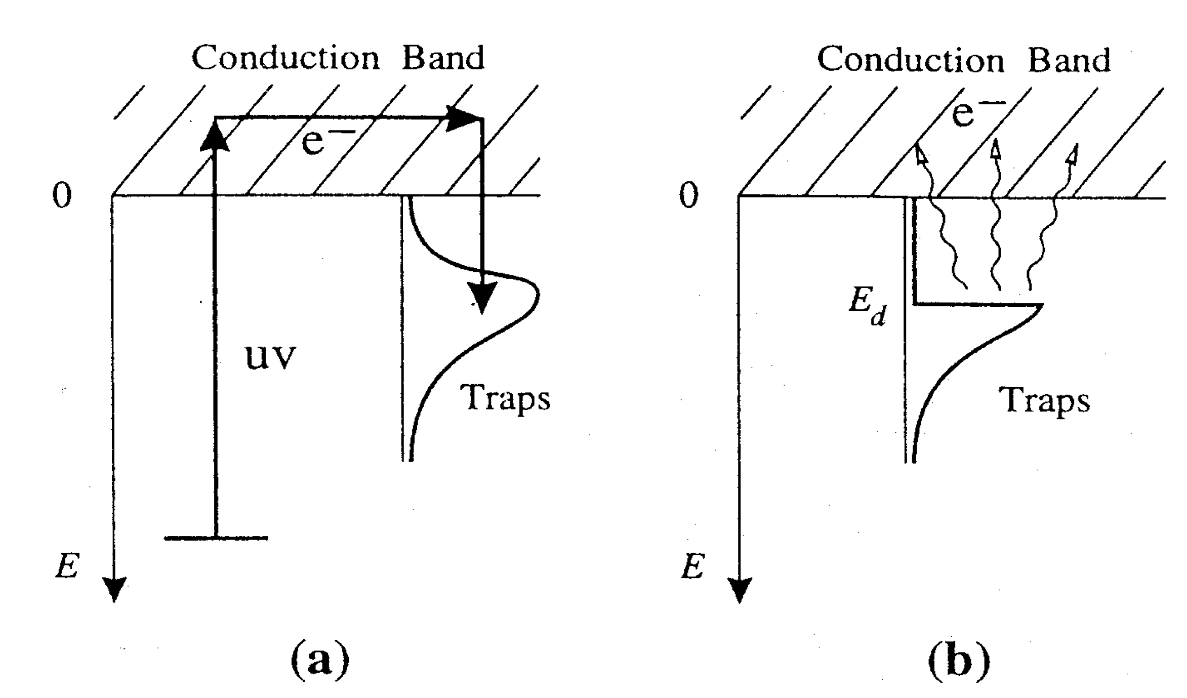
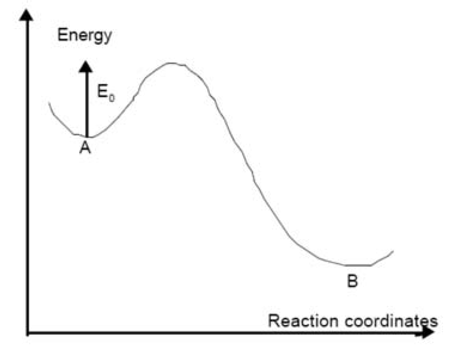
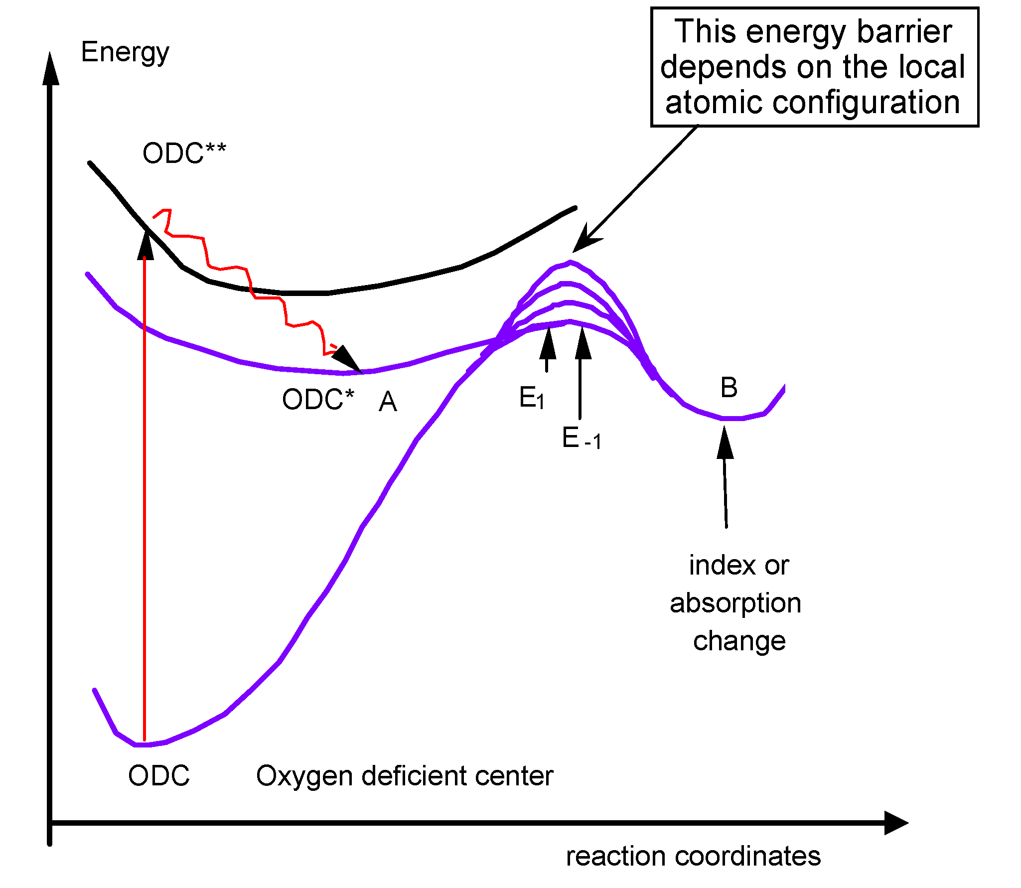
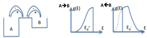
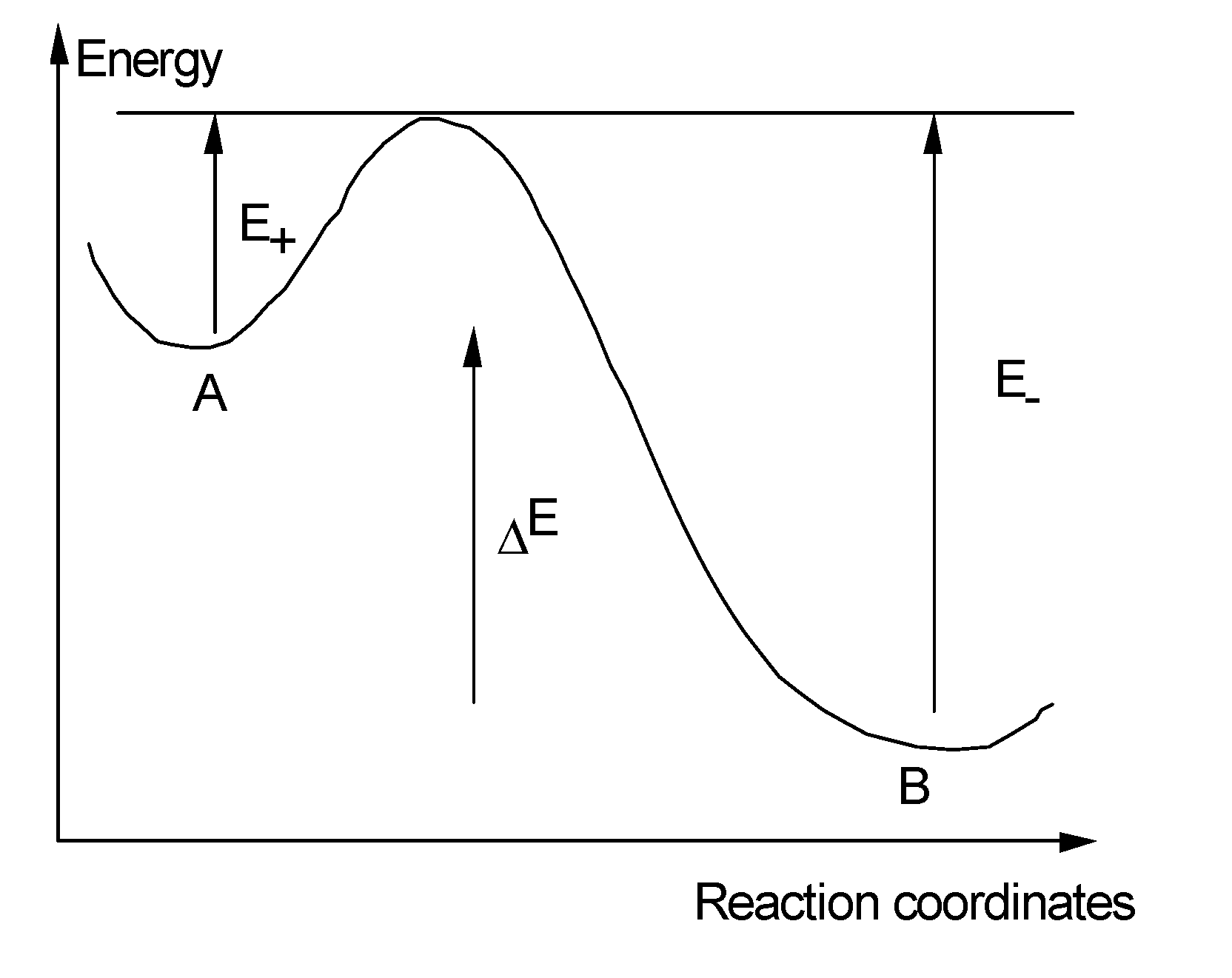
We can easily imagine that the reaction leading to refractive index change contains an absorption step on a species (for instance Oxygen Deficient Center), followed sometimes by a relaxation to another excited level (Figure 20). Then, several pathways are possible (one to luminescence, another one to bond breaking, migration, and structural rearrangement). All of them finally contribute to refractive index change. The first assumption we make here is that only one elementary reaction is involved: the limiting reaction of the process. We can write the reaction A→B.
Figure 20. Example of the absorption step of a physical chemical reaction, followed by a thermally activated reaction.
Fibers 03 00206 g020
(2)
The second assumption is that it is thermally activated (with an activation energy E). The Arrhenius law can be used, the d[B]/dt rate is proportional to a reaction constant k0 like k(E, T) = k0exp(−E/kBT), where kB is the Boltzman constant and [B] is the concentration of the B species.
(3)
The third assumption is that activation energy is distributed. As a matter of fact, in glasses, E is not unique. The creation energy of B can vary with its atomic environment. The transition state energy (the bottleneck on the reaction pathway) is also sensitive to the disordered environment in such a way that the activation energy, which is the energy difference between B and the transition state, is distributed. This means that chemical pathways are variable depending on the configuration distribution of the transition state and/or the initial stable states throughout the glass. This is at the origin of ergodicity lost because space-time points are no more equivalent. The reaction is faster in some places than in others. This is also heterogeneity, but not at a macroscopic level, just at a microscopic one.
We can call the relevant distribution g(E) and we chose to normalize it. If g is relevant to a thermal disorder, a Gaussian distribution seems likely. If g is relevant to a diffusional process, a Poisson distribution is better, but other approximations have also been used: differentiation of a sigmoid [1,17], and top hat function [5]. We will also see that g(E) can be obtained from the experiment and then approximated if necessary. At this step of the description, calling x the advancement of the reaction, depending on the activation energy E and the time, we have:
x ( E , t , T ) t ) E , T = k ( E , T ) ( 1 x ( E , t , T ) ) [ B ] ( t , T ) = A 0 0 x ( E , t , T ) g ( E ) d E
These assumptions constitute the first group of assumptions that are mainly connected to disorder.

2.2.2. The Assumption on the Reaction (Connection with Time and Temperature)

This assumption will allow computing the time dependence properly.
Most of the elementary reactions are first order, some are second order, when two species associate, but these are less likely. Thus, it is reasonable to assume that A→B is a first order reaction with a rate constant k(E, T) = k0exp(−E/kBT) (second order reaction is investigated in Section 5.1). This allows to compute the advancement degree x ( E , t , T ) = 1 exp ( k ( E , T ) t ) . Usually, the B integral is not analytically computable and, thus, extraction of g(E) is very difficult. A simplification of the integral is required to handle complex cases. Here, we can observe that x(E, t, T) is a very steep function of E, in such a way that, below a demarcation energy, Ed, x is equal to 1 and above Ed is equal to 0 (Figure 21). This clever remark, made by Vand [28], leads to a useful simplification of the equation:
[ B ] ( t , T ) = A 0 0 E d ( t , T ) g ( E ) d E = [ B ] ( E d )
We note that B content appears to depend now only on Ed.
To define Ed properly, we can chose the value where x(E)t,T varies the most (the steepest variation defined by 2 x E 2 ) t , T ( E = E d ) = 0 , in this case, we get Ed = kBTln(k0t).
Figure 21. Comparison of widths between x(E, t, T) and the distribution g(E).
Fibers 03 00206 g021
Remarks and consequences of the theory:
(1)
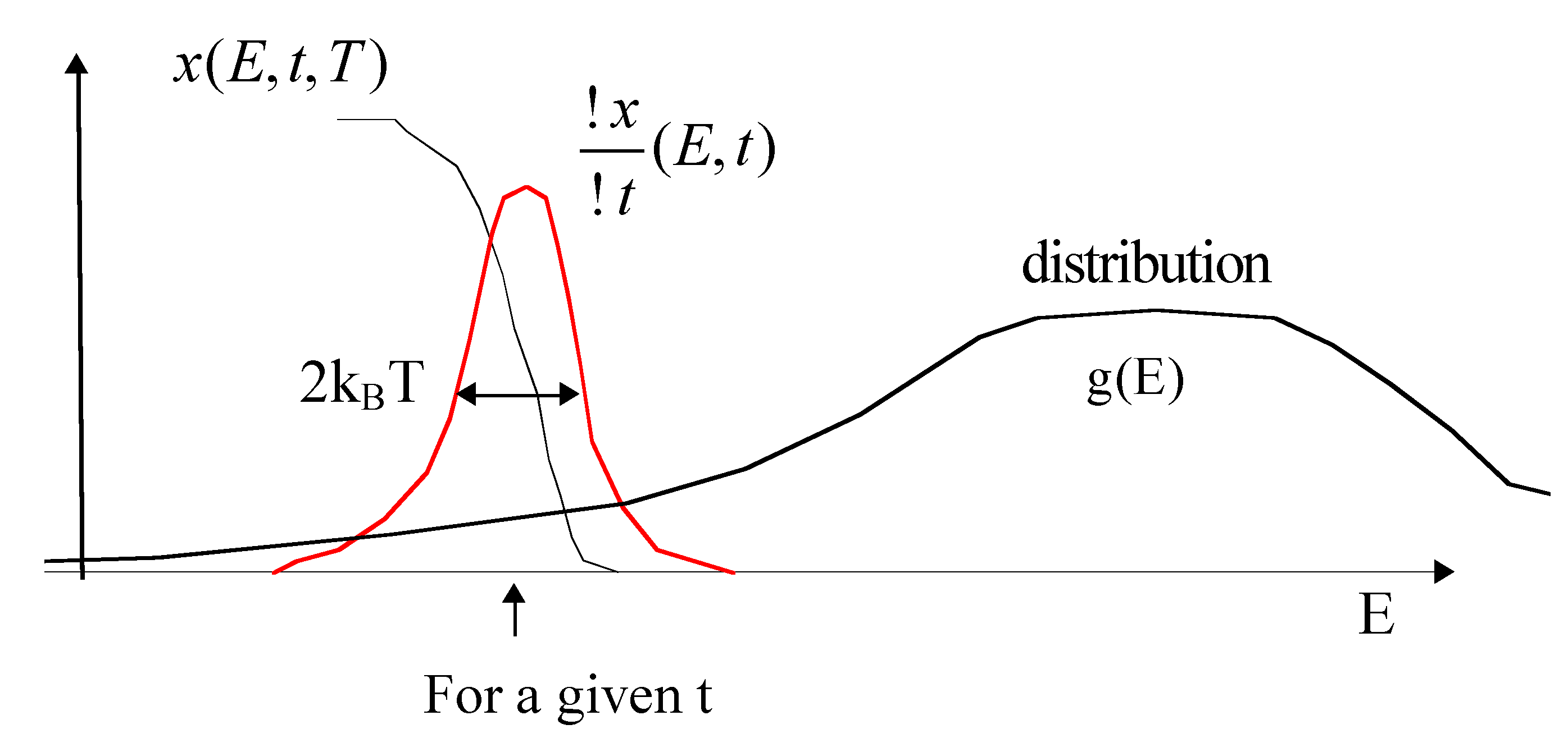
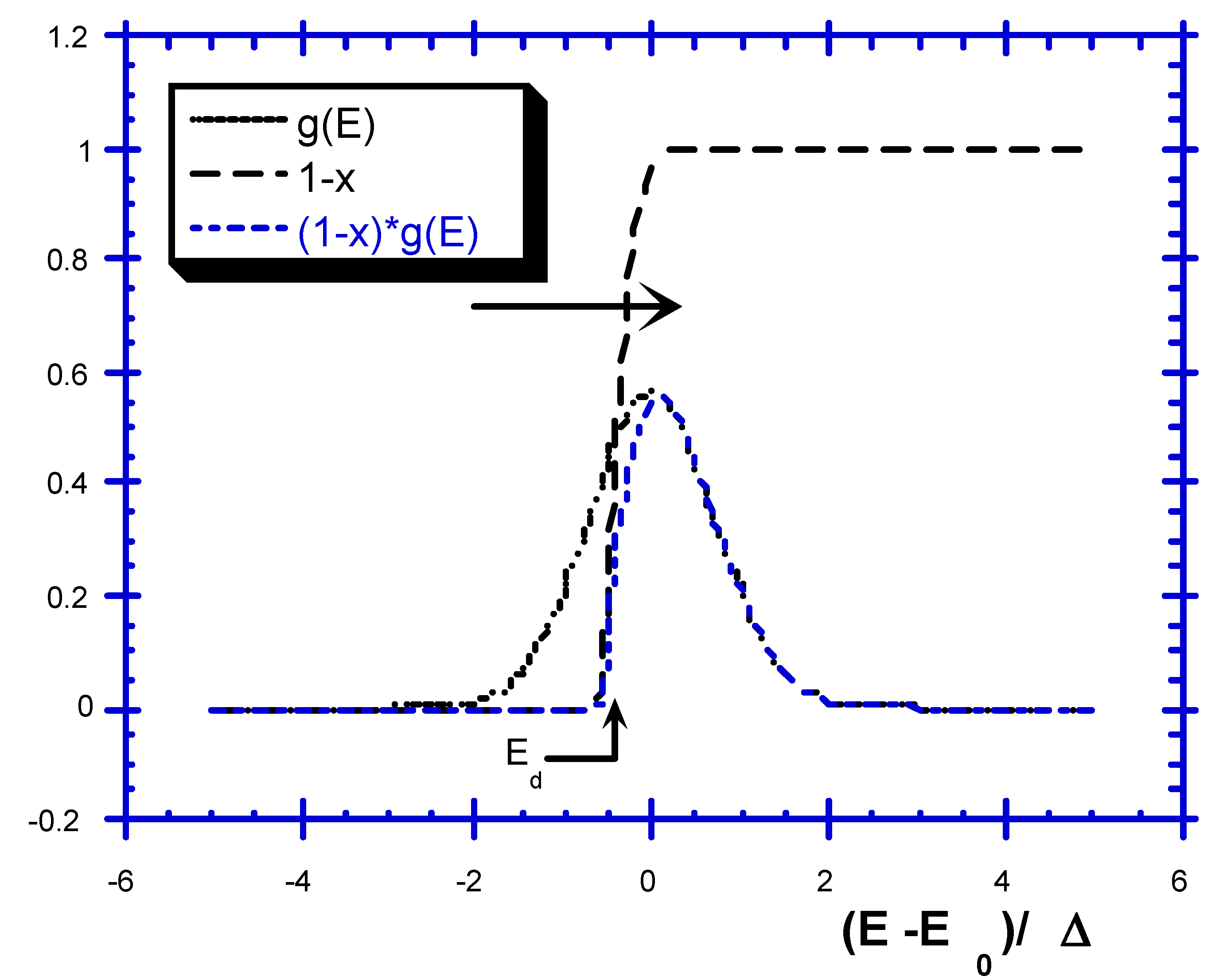
It is worth noting that the reaction properties appear now only in Ed(t, T), on one hand (the bound of the integral), and, on the other hand, the structural disorder appears in the integrand.
(2)
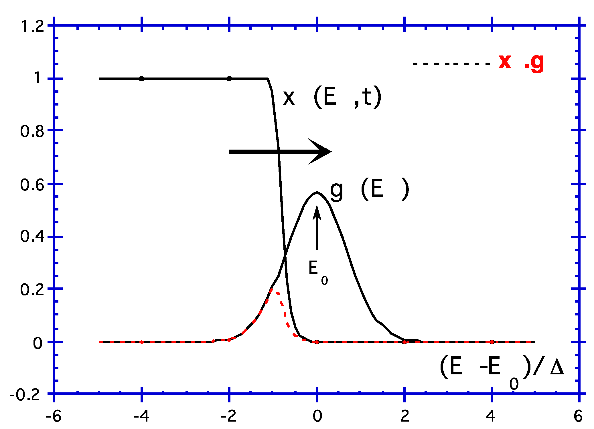
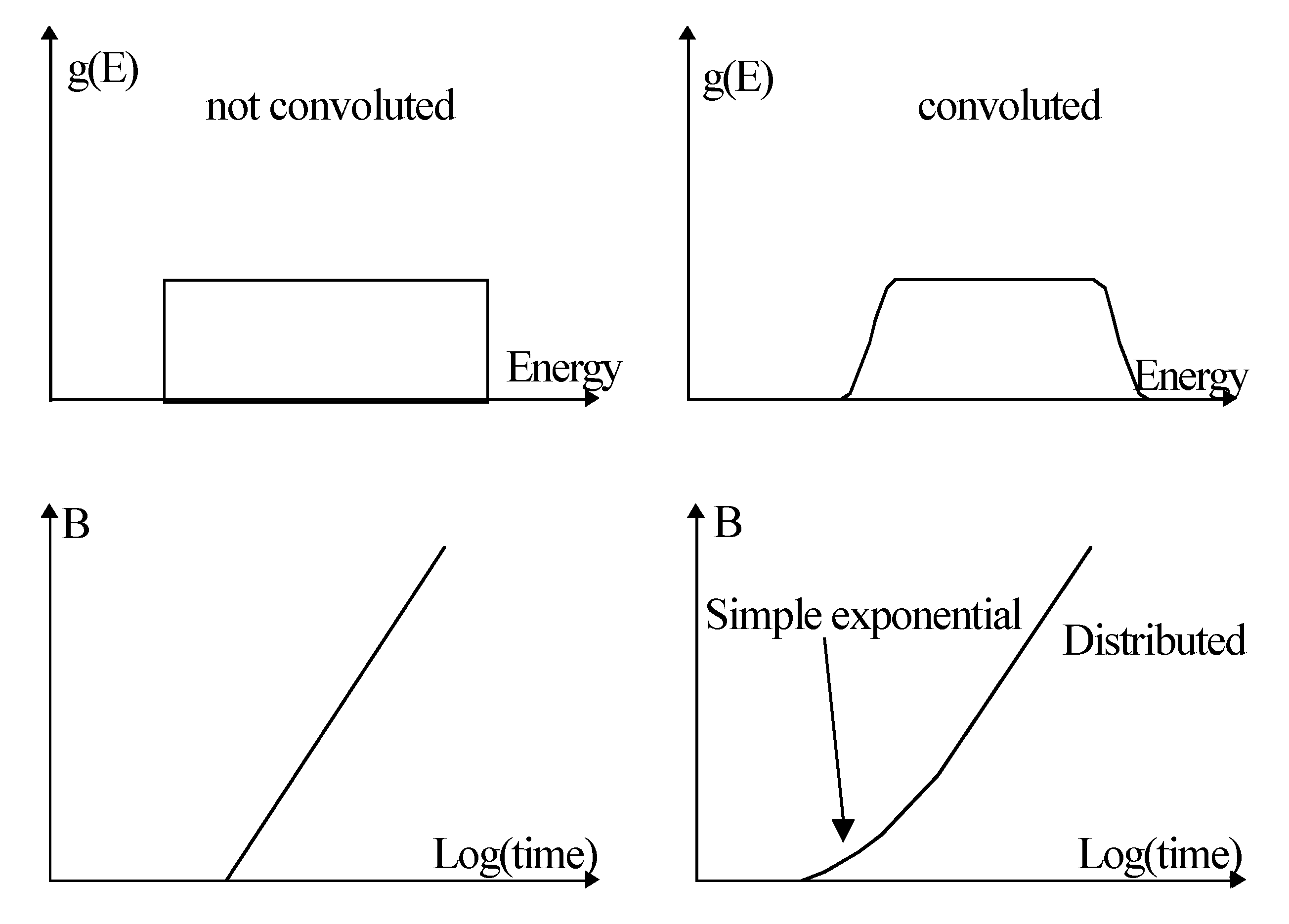
Note that the demarcation energy approximation is valid only if g(E) varies slower than x(E, t, T). The width of x ( E , t , T ) E ) t , T is 2kBT. Otherwise, a correction has to be added to the integral [32]:
k B T k = 0 k = c k + 1 d k g ( E ) d ( E / k B T ) k | e = e d
where ck+1 are constant close to unity (c1 = Euler constant 0.577, c2 = 0.989, c3 = 0.907, c4 = 0.981, c5 also and then equal to 0.999).
(3)
Most interesting, the differentiation of B against Ed( d B d E d = A 0 g E d ) yields the shape of the distribution function.
(4)
As B is expressed with only one variable B(Ed). It exhibits the same shape as B(T) for given t or B(ln(t)) for given T. Thus, we deduce that if g(E) does not depend on T, isochrons and isotherms are equivalents:
For isotherms Δn should be measured at the same temperature.
For isochronous annealing, there is a criterion in the temperature step and duration of the step (see Section 4.2).
For a given time, [ B ] ( t , T ) is the area under the dotted curve as in Figure 22. As t increases, x moves to the right hand side and more difficult pathways are used.
Figure 22. Progress of advancement degree along the distribution function.
Fibers 03 00206 g022

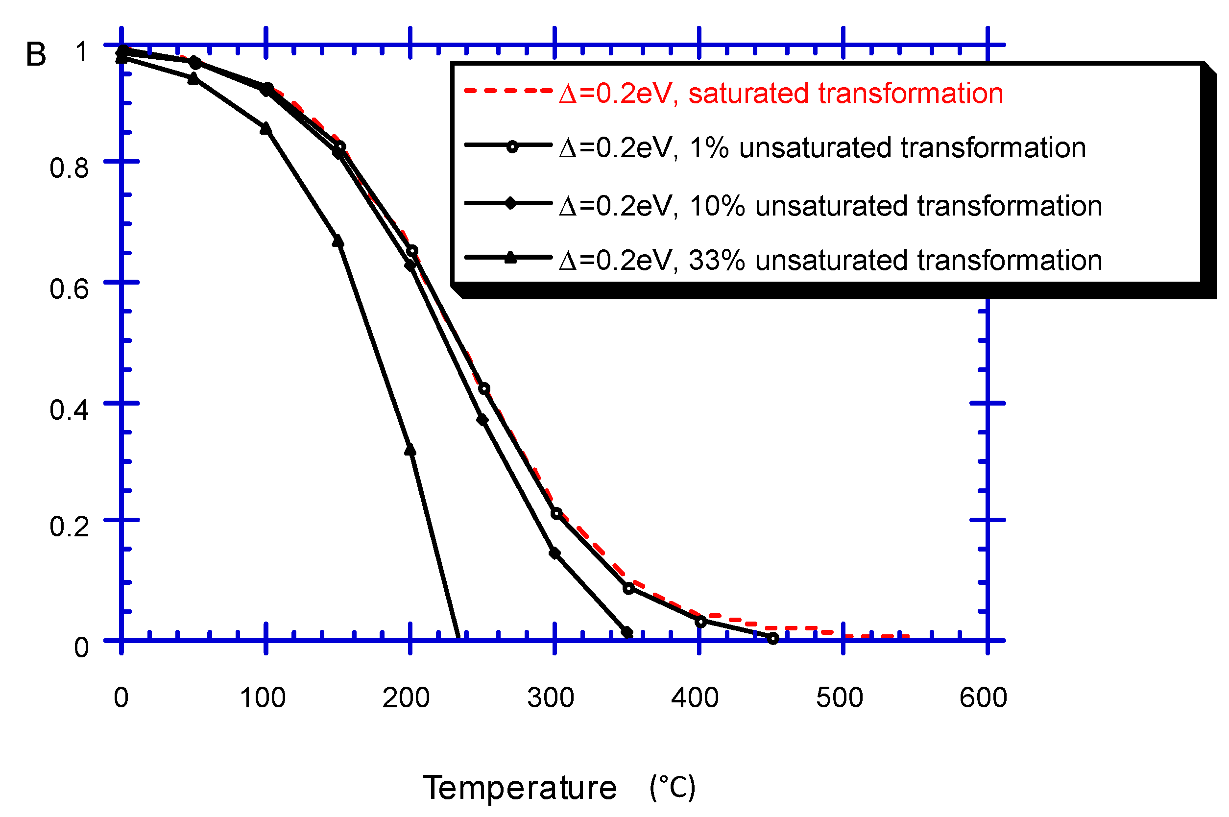
2.2.3. Examples for Time Dependence Computation

(Step 1)
Integration using a Gaussian distribution as the following:
g ( E ) = 1 Δ π exp ( ( E E 0 Δ ) 2 )  with  E 0 2 Δ  centered on  E 0 ; width  Δ
yields:
[ B ] ( t , T ) = A 0 1 Δ π 0 E d ( t , T ) exp ( ( E E 0 Δ ) 2 ) d E [ B ] ( t , T ) = A 0 2 [ 1 f e r r ( E d E 0 Δ ) ] ,  where  f e r r  is the error function
(Step 2)
The integration of a sigmoid differentiation distribution:
g ( E ) = 1 k B T 0 exp ( E E 0 k B T 0 ) ( 1 + exp ( E E 0 k B T 0 ) ) 2
yields:
[ B ] ( t , T ) = A 0 0 E d ( t , T ) g ( E ) d E = A 0 exp ( E d ( t , T ) E 0 k B T 0 ) 1 + exp ( E d ( t , T ) E 0 k B T 0 ) = A 0 ( k 0 t ) T T 0 exp ( E 0 k B T 0 ) 1 + ( k 0 t ) T T 0 exp ( E 0 k B T 0 )
(Step 3)
with a Poisson distribution:
g ( E ) = 1 k B T 0 exp ( E k B T 0 )
We obtain:
[ B ] ( t , T ) = A 0 0 E d ( t , T ) g ( E ) d E = A 0 [ 1 exp ( E d ( t , T ) k B T 0 ) ] = A 0 [ 1 ( k 0 t ) T T 0 ] and T < T 0

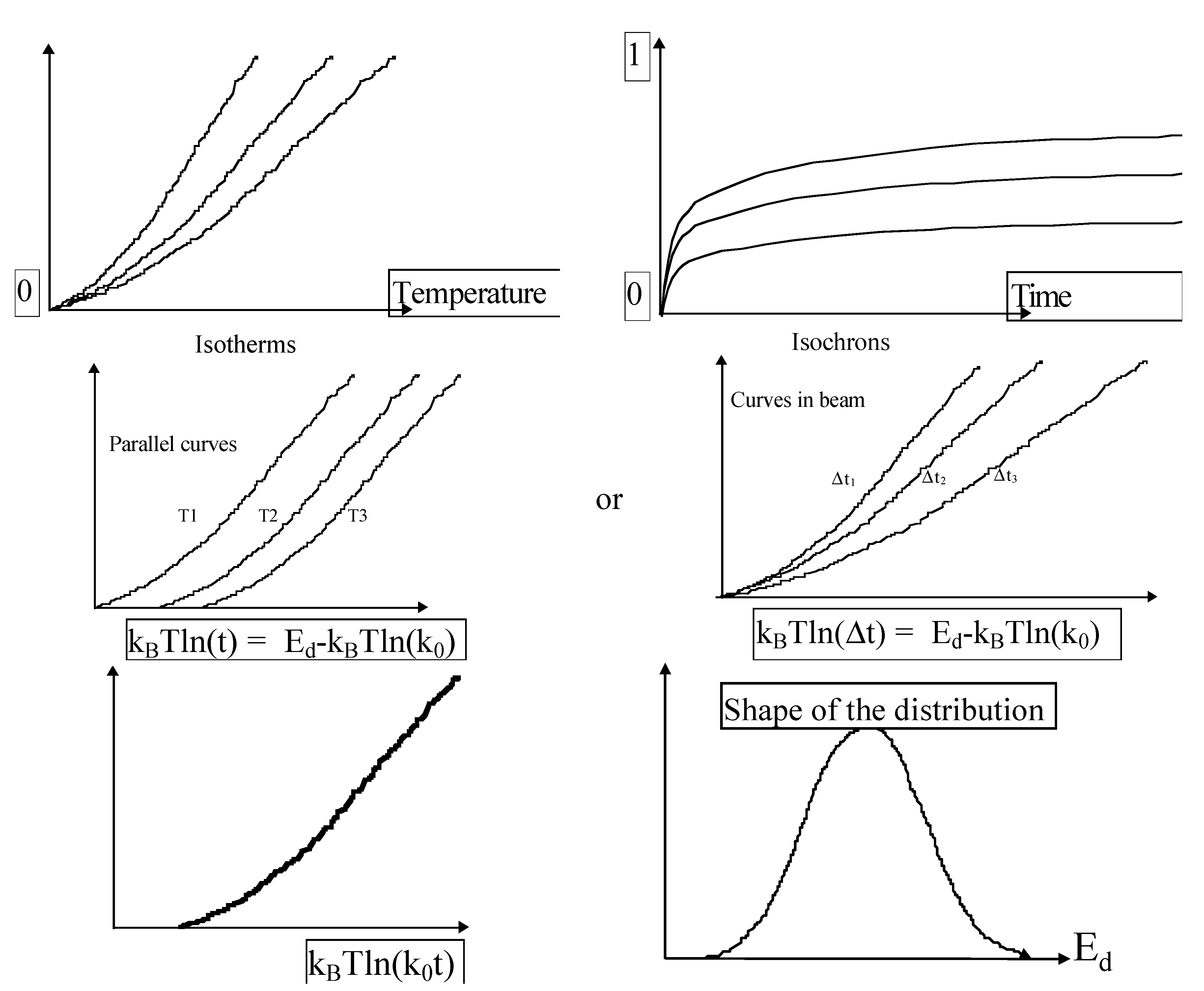
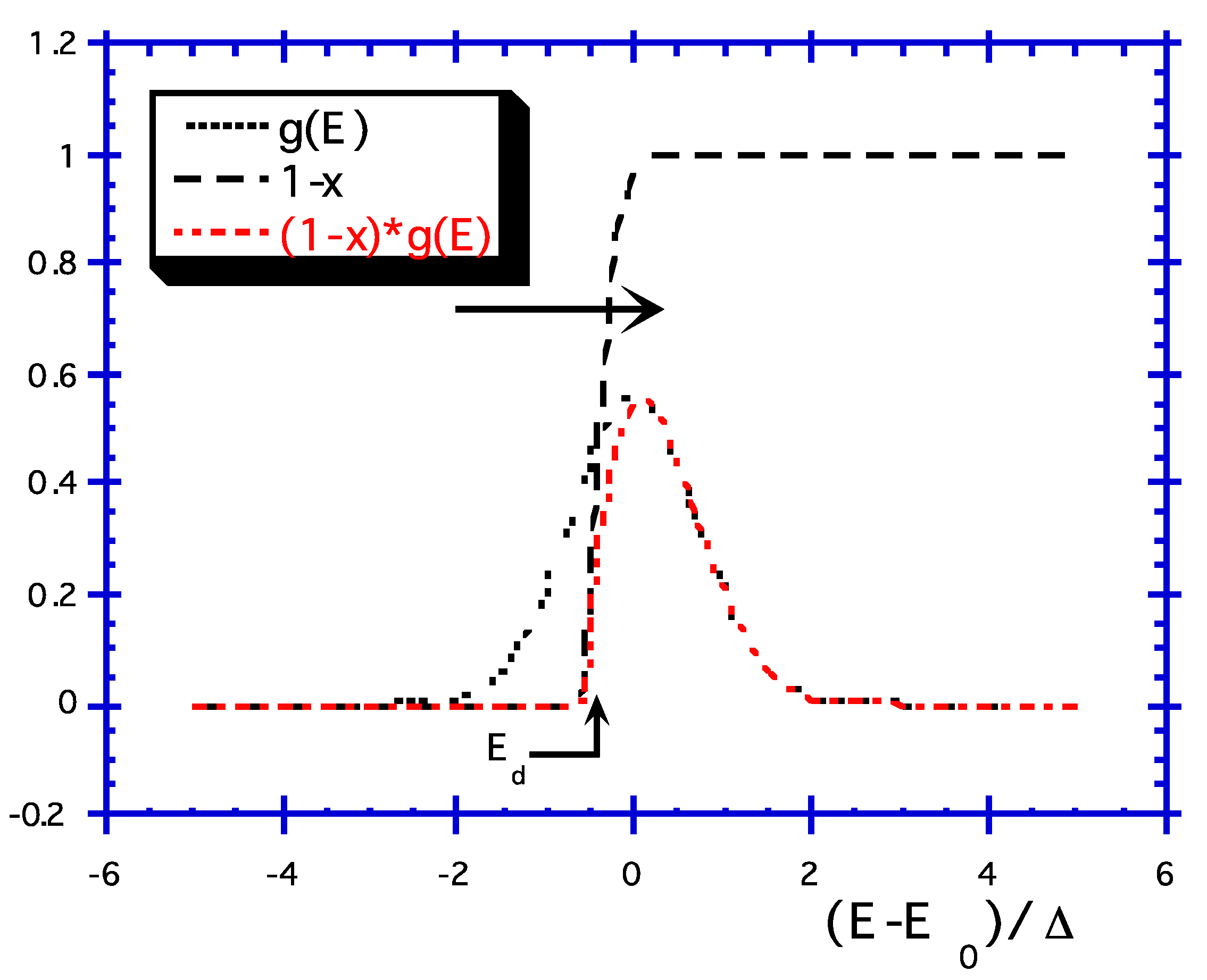
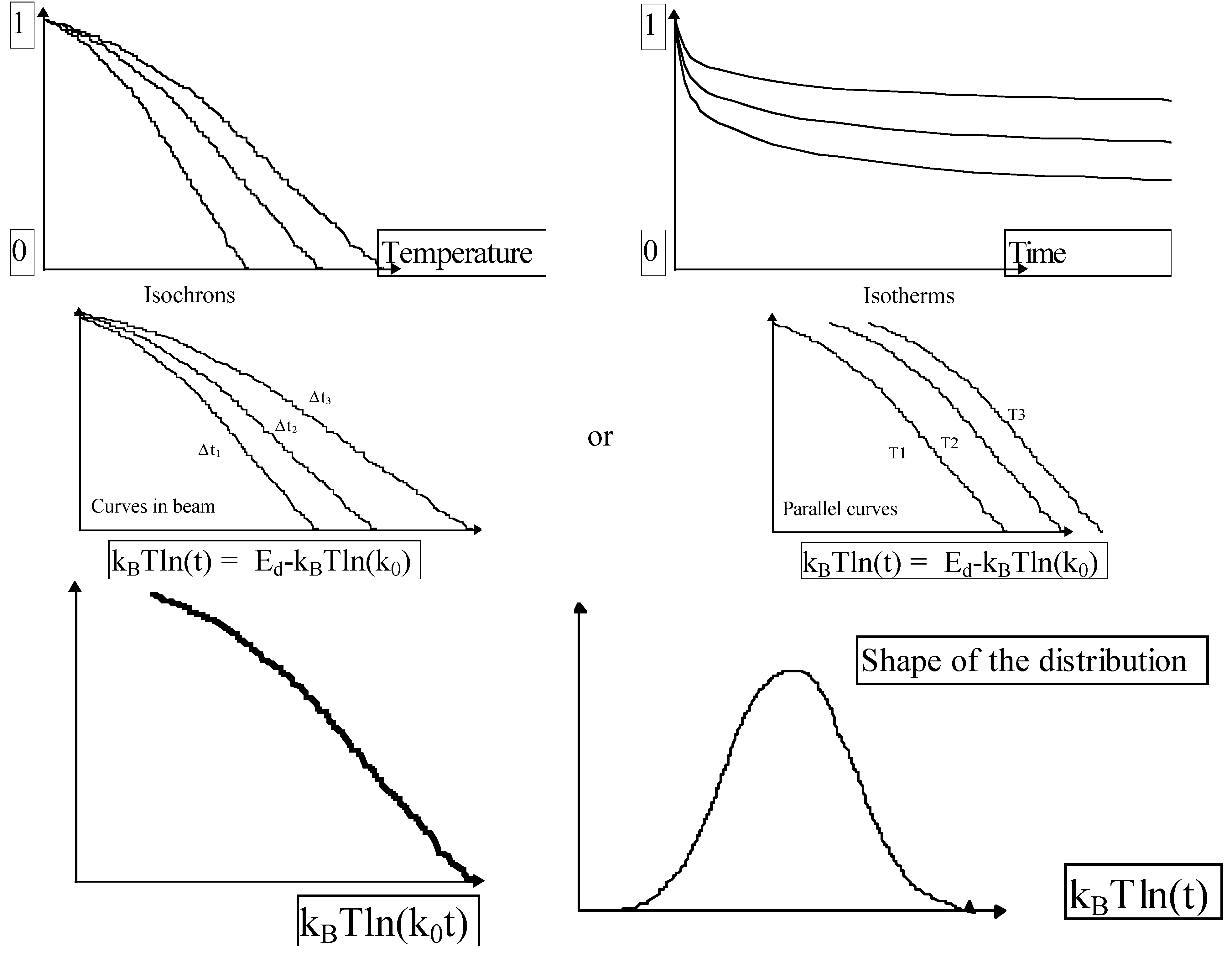
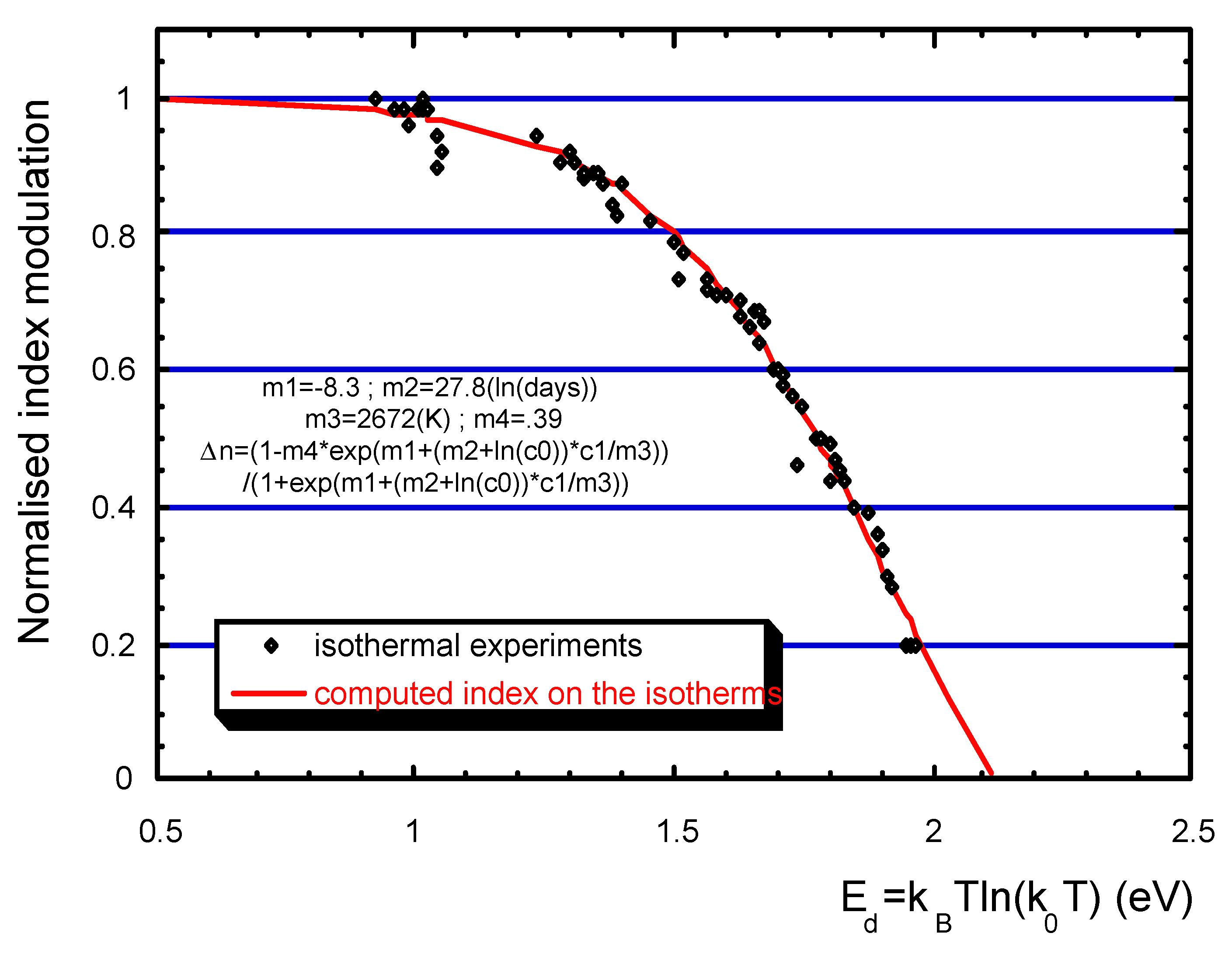
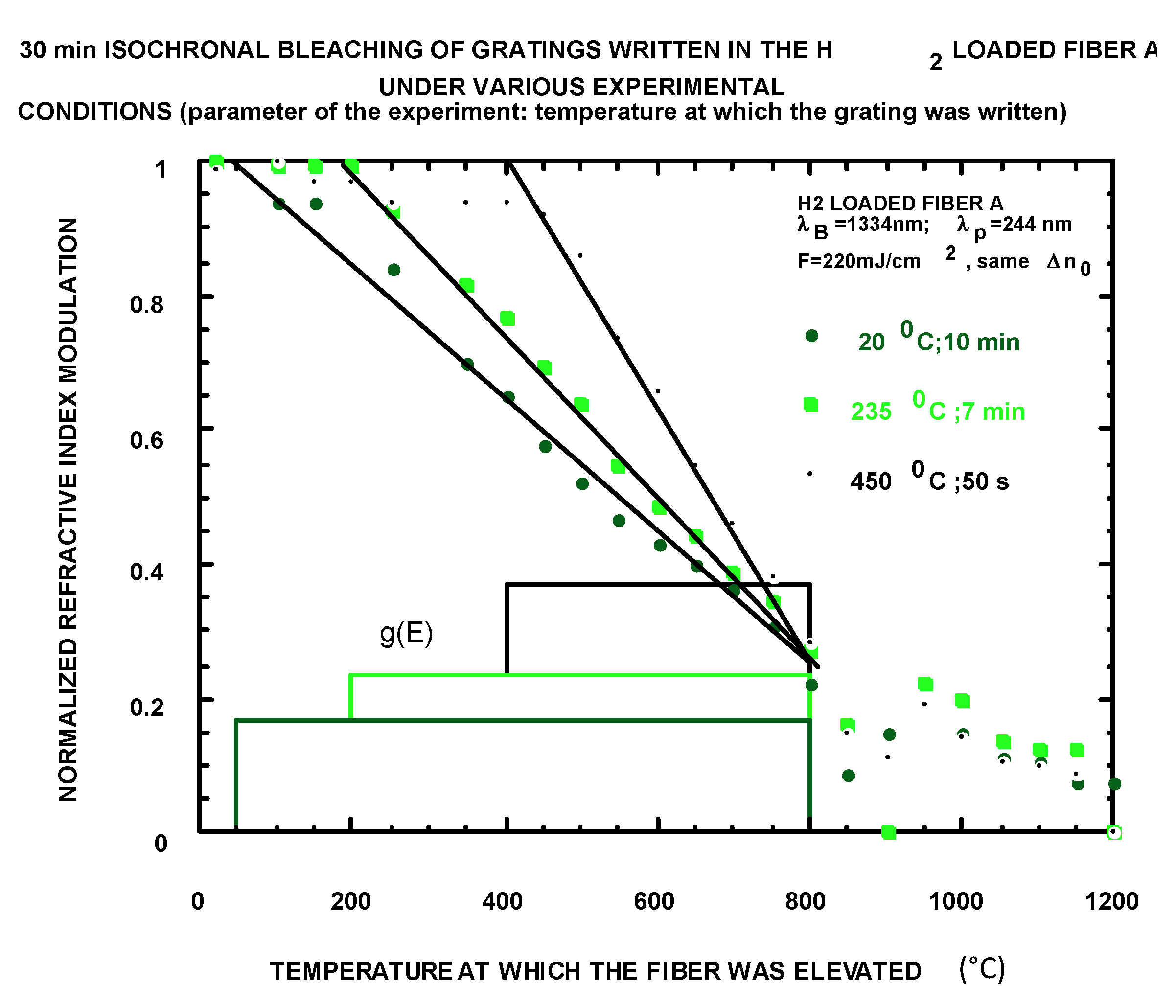
2.2.4. How to Obtain k0 and g(E) (Figure 23)

(1)
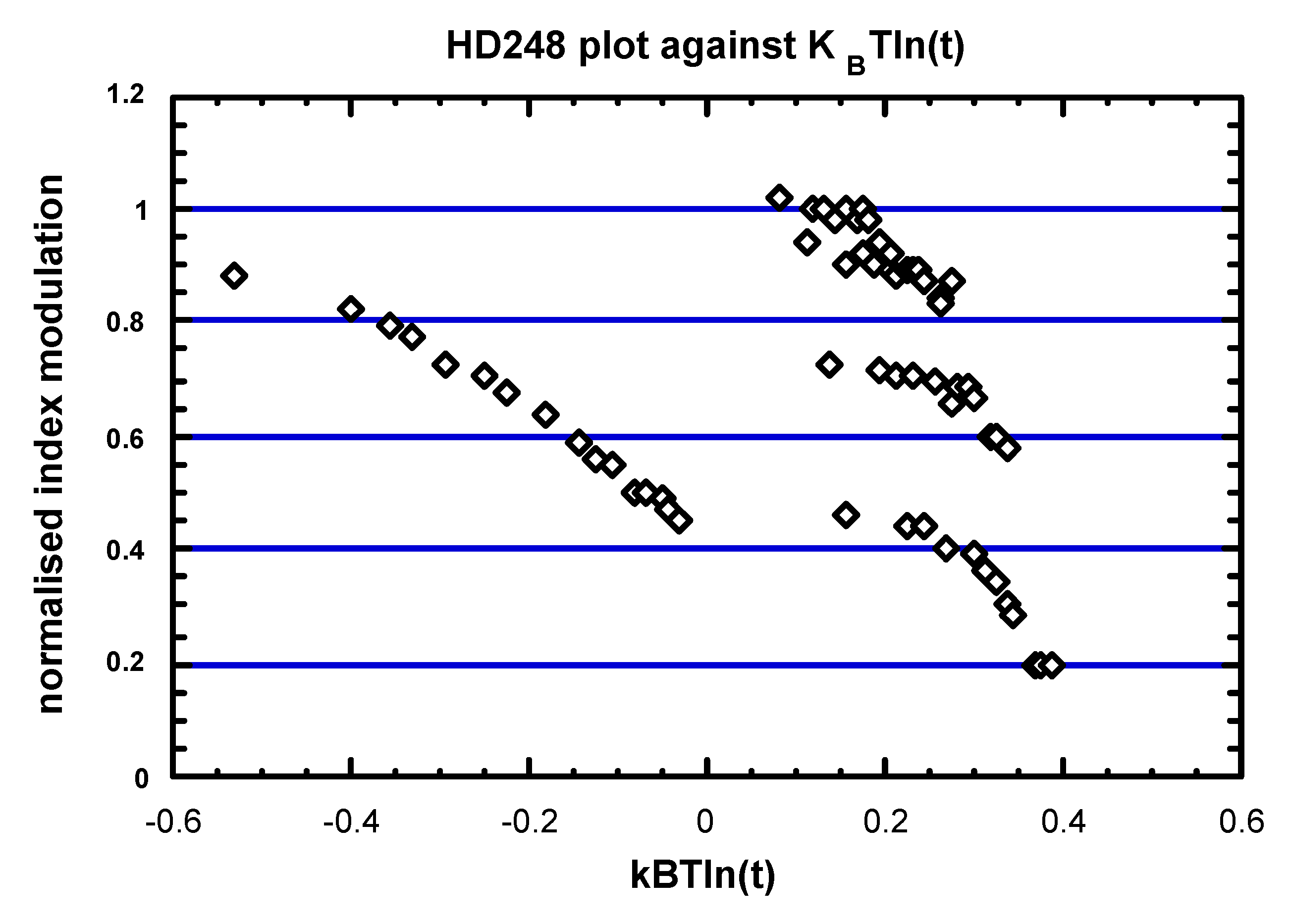
Measurement of several isochrons or isotherms writing kinetics and replotting against a new abscissa;
(2)
k0 fitting for curve collapsing and;
(3)
Differentiation [ B ] ( E d , T ) E d ) T = A 0 g 1 ( E d ) .
Figure 23. Procedure to obtain k0 and g(E).
Fibers 03 00206 g023
We can note that k0 and g(E) are determined separately. The first one is related to the order of the kinetics and the second one is a measurement of the disorder of the glass.

2.3. Kinetics of Erasing

The hypotheses for modeling the relaxation behavior, i.e., the erasure (A←B), are basically the same as for the forward reaction (A→B). There is a symmetry in the approach. The only difference is that the starting population is different. Whereas all sites are under A form for a forward reaction, it may be under A or B form for relaxation, i.e., the writing has not transformed all A content, but only the easiest part (non-saturated writing). When the writing of the kinetics is completed, or is not distributed, the same computation as Section 2.2 applies in replacing A by B and vice versa, and, considering that the activation energy is for the backward reaction, the distribution is different (see below).
Otherwise, it is necessary to consider a starting distribution for B that is equal to A 0 x + ( E + , t w , T w ) g + ( E + ) = B 0 ( E + , t w , T w ) , i.e., the advancement degree times the distribution function for writing the reaction with tw, Tw the time and temperature of writing. We have to consider the following expression for B content, at time t, and at temperature T when forward pathways are independent of backward pathways.
[ B ] ( t , T ) = A 0 0 0 x + ( E + , t w , T w ) ( 1 x ( E , t , T ) ) g + ( E + ) g ( E ) d E d E +
This is equivalent to:
[ B ] ( t , T ) = A 0 0 x + ( E + , t w , T w ) g + ( E + ) d E + B 0 ( t w T w ) 0 ( 1 x ( E , t , T ) ) g ( E ) d E
Therefore, the same approach as Section 2.2 can be used again for solving this integral. Otherwise, when forward and backward reactions use the same pathways, the energy of the reverse reaction can be related to energy of the forward reaction and B0(E+) becomes B'0(E).
Let us now recall the methods of computation that are applicable to all cases.

2.3.1. First Group of Assumptions

(1)
One elementary reaction A k B (limiting process), A→B is the writing process;
(2)
Thermal activation, E, k ( E ) = k 0 exp ( E / k B T ) ;
(3)
E is distributed, i.e.,
-
variable chemical pathways;
-
the saddle point or the B state are sensitive to various structural configurations as decrived in Figure 24;
-
g(E) is the distribution function for backward reaction, it can be Gaussian for a thermal disorder or Poisson for a diffusional disorder or differentiation of a sigmoid, or also top hat function.
The total B content can be expressed as:
[ B ] ( t , T ) = 0 B 0 ( E ) [ 1 x ( E , t , T ) ] g ( E ) d E
B0(E) is the initial distribution of occupied sites according to the activation energy, regardless of the distribution functions, independent or not. 1 − x is the degree of retardation.
Figure 24. Reaction pathway for reverse reaction.
Fibers 03 00206 g024

2.3.2. Second Group of Assumptions (towards the Computation of Time Dependence)

For computing the time and temperature dependences of the B content ([B](t, T), we have to make the following assumptions:
(1)
Most of the elementary reactions in solids are first order; some are second order, when two species associate, but these are much less likely. Thus, this is not so severe and we can write: A k B , d x - d t = k ( 1 x ) , x ( E , t , T ) = 1 exp ( k ( E , T ) t ) is the advancement degree of the reaction.
(2)
Concept of demarcation energy, Ed
x ( E , t , T ) is a function that varies very quickly with E. B0(E) is the initial population, produced by the FBG writing.
x ( E , t , T ) { = 1                     for low energies (reaction completed) = 0       for high energies (reaction did not begin)
When x(E, t, T) varies faster than g(E), it can be approximated to a Heaviside function at energy Ed and, thus, we can read:
[ B ] T ( t , T ) = 0 B 0 ( E ) exp ( k ( E , T ) t ) g ( E ) ) d E = E d B 0 ( E ) g ( E ) d E
Ed is properly defined by 2 x E 2 ) t , T ( E = E d ) = 0 . For a first order reaction, E d = k B T ln ( k 0 t ) . The reaction properties (i.e., k 0 ) are only appearing in Ed, the disorder (relevant of the glass) appears in g(E). Finally, [B](t, T) is the area under the red dotted curve in Figure 25. The retardation degree 1 − x(E, t, T) in the progression erases the B distribution.
Figure 25. Reaction progresses by removing B sites, from less stable to the most stable sites.
Fibers 03 00206 g025
  • Some Consequences of the Theory:
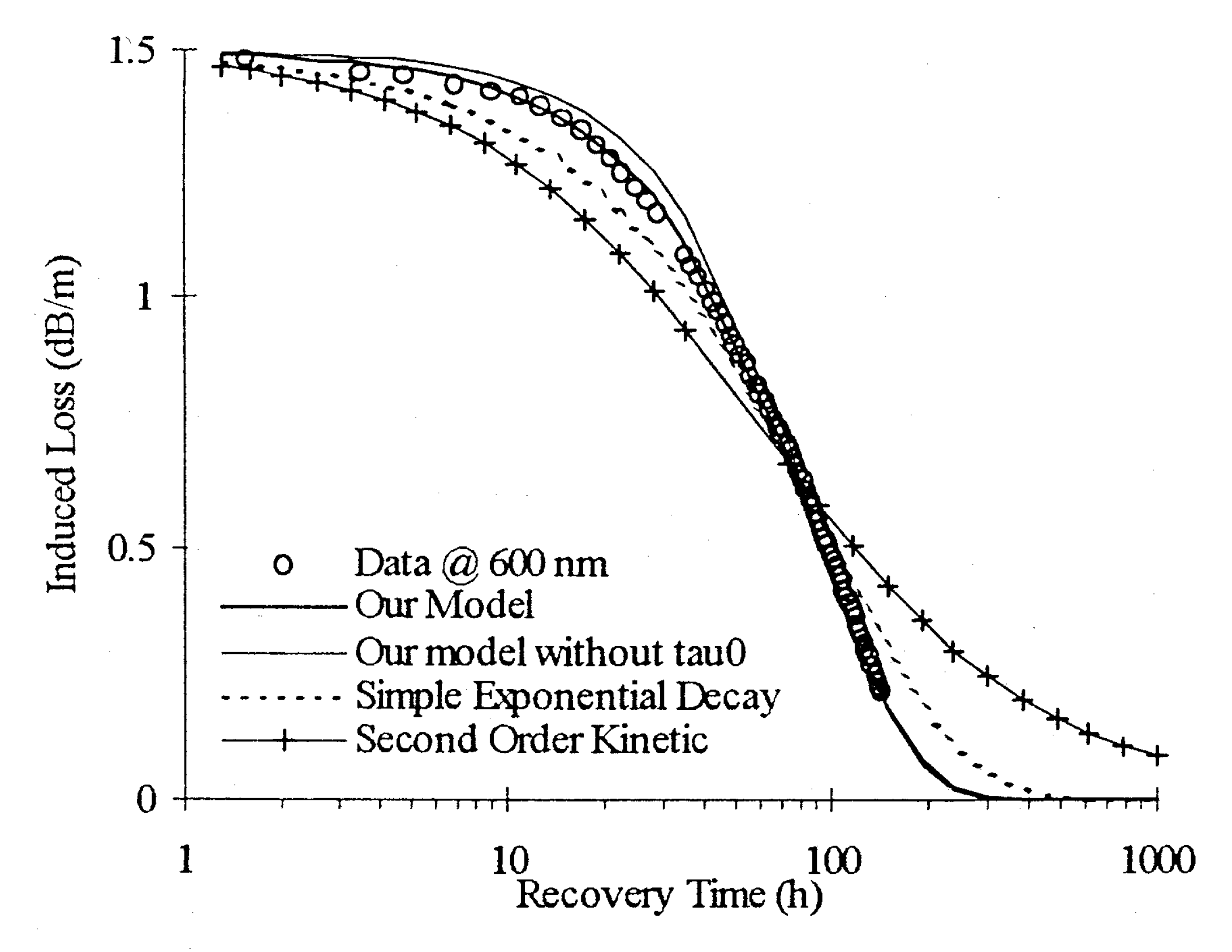
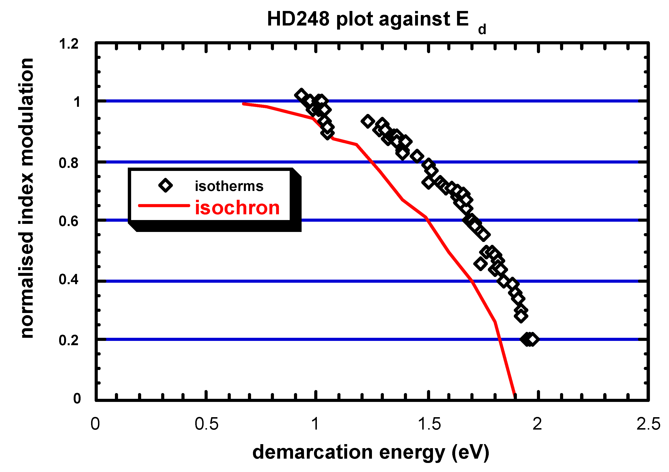
    (1)
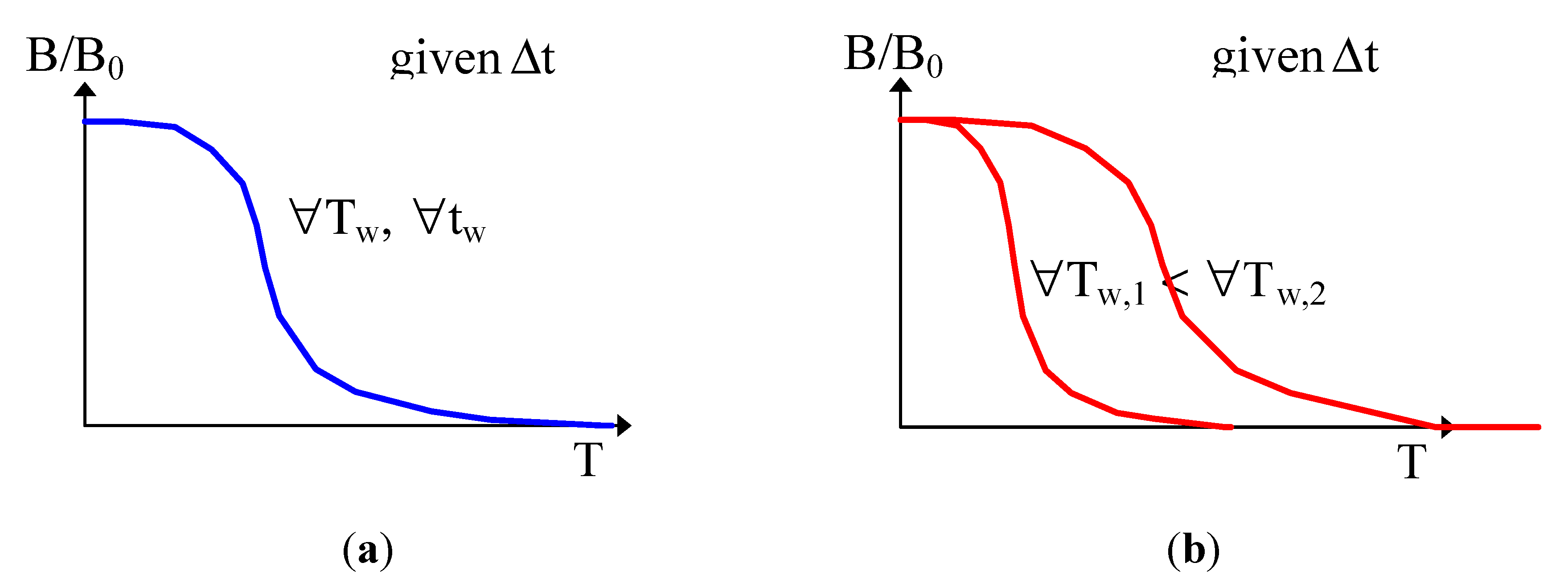
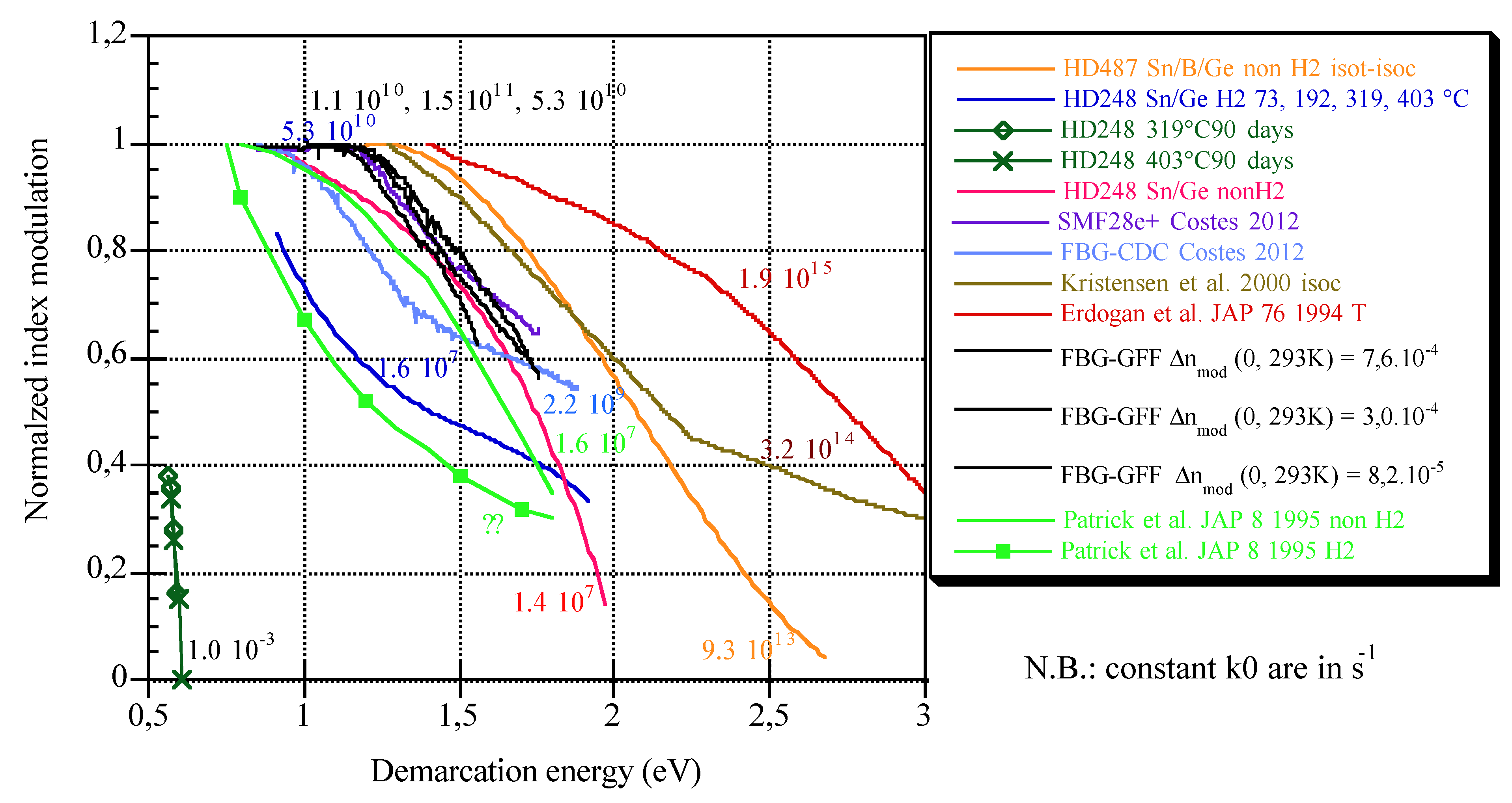
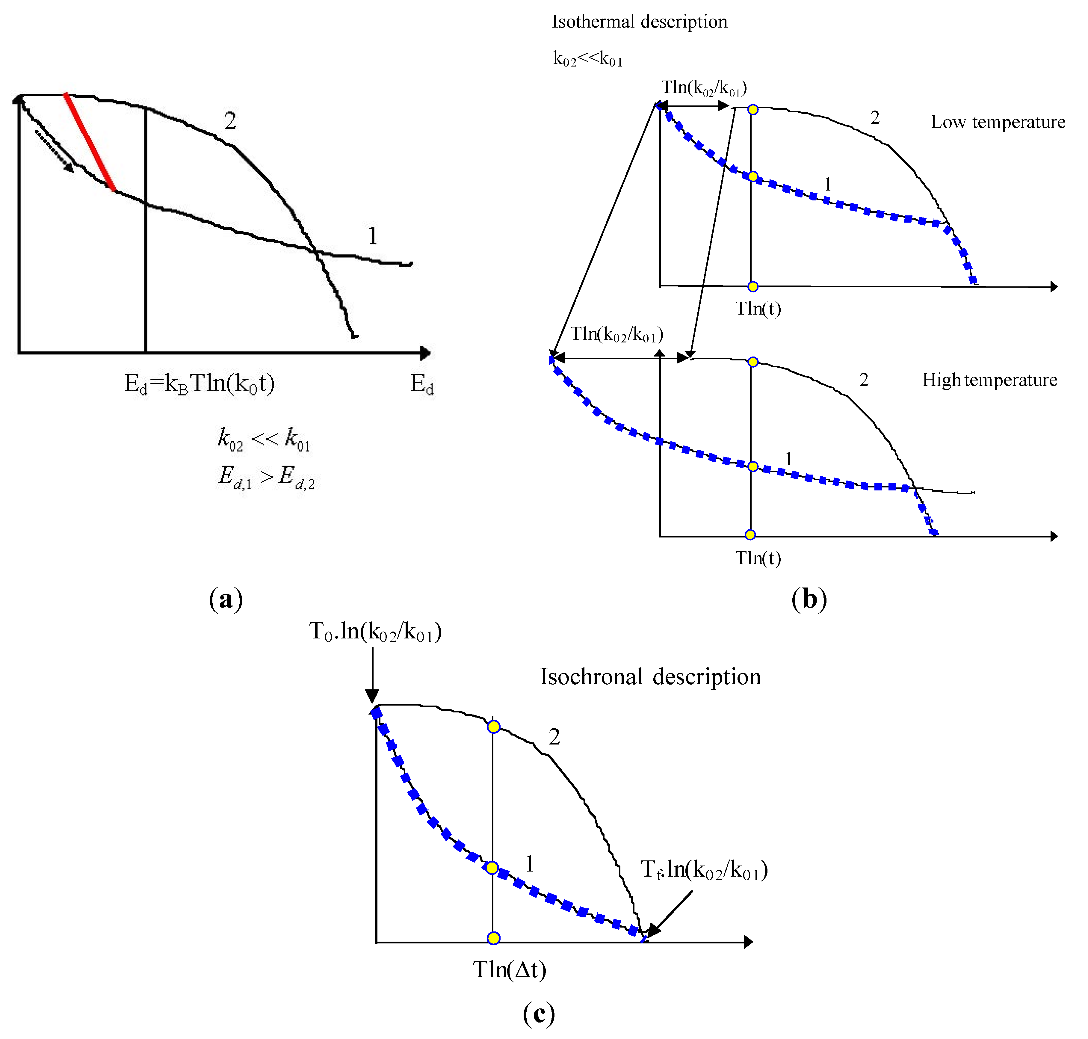
    [B](t, T) can be expressed as a function of the unique variable called demarcation energy ( E d ). The curve [ B ] ( E d ) is called the master curve (MC), as it is unique, regardless of what the (t, T) couple may be for a given value of Ed. We can note that T is equivalent to lnt in E d and, thus, isochronal ageing data are equivalent to isothermal ageing data for establishing MC. Note that from a practical point of view, most people consider that NICC( E d ) is the master curve. Now, the MC plot allows the user to predict the grating lifetime, providing that the anticipated conditions of BG (i.e., E d = f(tuse, Tuse) correspond to a point on the MC that has been actually sampled during the annealing experiment.
    (2)
    Notice also that the distribution function is included in the MC differentiation as: d [ B ] d E d = B 0 ( E d ) g ( E d ) .
    (3)
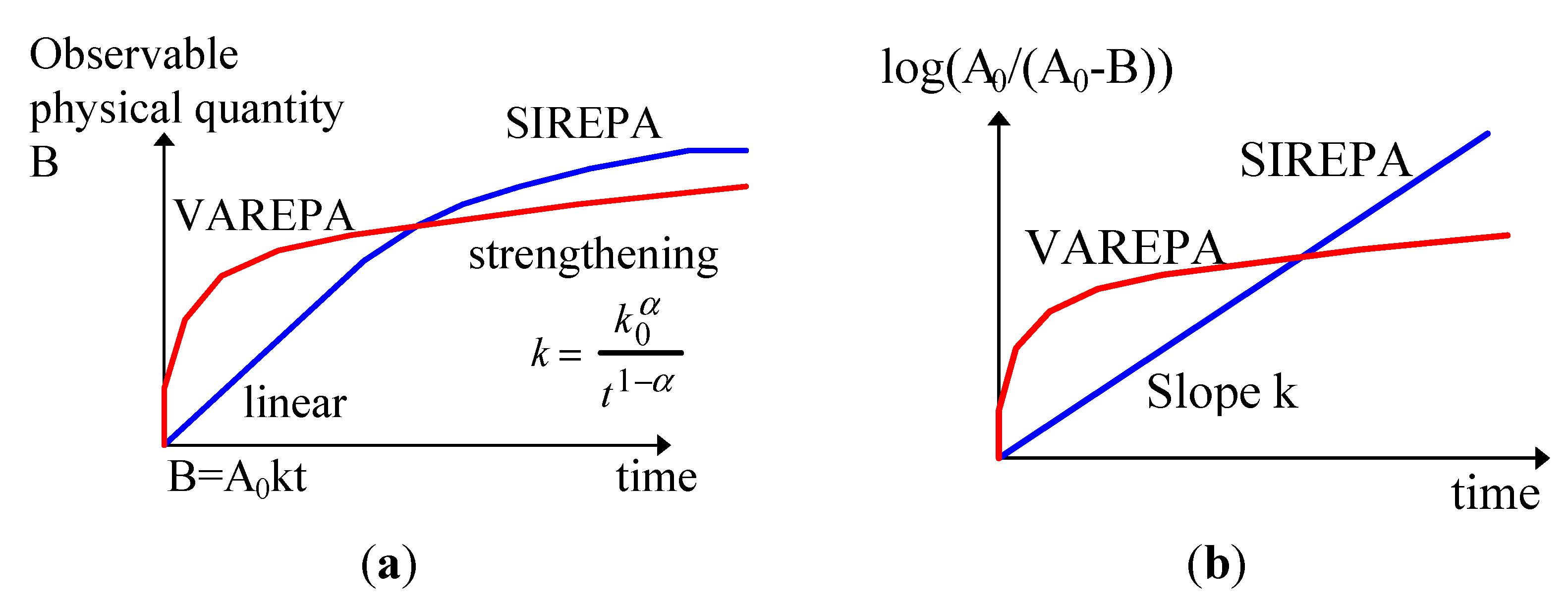
    Thermal stability increases along with the ageing time (hardening). This is due to the fact that the less stable sites are removed along the ageing.
    -
    (1) When the pathways are the same in both senses, the distribution function is the same for forward and backward reactions, as shown in the scheme below. If the writing kinetics are not saturated, the forward distribution function is not saturated and, thus, neither is the backward distribution. The stability is dependent on the writing (time and power density that is included in k 0 + , see B0(Ed) in definition)
    Fibers 03 00206 i001
    -
    (2) When there is no correlation between the distribution functions because the pathways are not the same, there are two independent distribution functions, as shown in the scheme below. The B sites are randomly occupied whatever its stability. The complete distribution function of the backward reaction has to be used. The stability is independent of writing (i.e., on the initial grating strength), see Section 2.3.3.
    Fibers 03 00206 i002

2.3.3. A Few Examples of Time Dependence Computations Assuming B0(E) = B0

If g-(E-) is Gaussian then:
[ B ] ( t , T ) = B 0 ( 1 f e r r ( k B T ln ( k 0 + t ) E 0 Δ ) 2 ) B 0 ( 1 a ( k + 0 t ) k B T Δ ) for low  t
If g-(E-) is a Poisson distribution then: [ B ] ( t , T ) = a ( k + 0 t ) k B T Δ ; Δ is the width of the distribution.
If g-(E-) is a differentiation of a sigmoid then: [ B ] ( t , T ) = B 0 ( 1 1 + a ( k + 0 t ) 3 k B T Δ )
If g-(E-) is a top-hat of width Δ then: [ B ] ( t , T ) = B 0 ( E max k B T ln ( k + 0 t ) Δ ) , etc.

2.3.4. Incomplete forward Reaction in the Case of Dependent Backward and Forward Pathways (B0(E)) [36]

If there is dependence between the writing and the relaxation, the distributions are the same but shifted in energy, it is, in this case, valuable to know the relationship between E+ and E. We can solve the problem rather easily when the forward and backward reactions use the same pathways. In this case, EE+ = ΔE where ΔE is the formation energy difference between A and B (Figure 26).
Figure 26. Relationship between activation energies.
Fibers 03 00206 g026
We consider the initial distribution of B, B 0 ( E + , t w , T w ) = A 0 [ 1 exp ( k ( E + , T w ) t w ) ] in the following integral B ( t , T ) = 0 B 0 ( E + , t w , T w ) exp [ k ( E , T ) ] g ( E ) d E .
Hypothesis: the forward and backward pathways are the same ≥ EE+ = ΔE
A k B k = k 0 exp ( E k B T )
For each E, x ( E , t ) = 1 exp [ k ( E ) t ] .
B ( t , T ) = A 0 0 [ 1 exp ( k + ( E + , T w ) t w ] define  E d + exp ( k ( E , T ) ) define  E d g ( E ) d E
in the scale of E, we define Ed+' = Ed+ + ΔE, considering that each E+ is related to an E, which is E+ + ΔE. This means that the function 1 − exp(−k+t) switching at E+d in the E+ scale commutes at E+d + ΔE in the scale of E, i.e., there is no more B above this value or there is no reverse reaction above E+d + ΔE (Figure 27), thus B ( t , T ) = A 0 E d E d + + Δ E g ( E ) d E = A 0 E d Δ E E d + g + ( E + ) d E + .
Figure 27. Erasure of incomplete distribution.
Fibers 03 00206 g027
We can note that the stability increases with an increase of tw or Tw because E+d increases, leading to the occupation of more stable sites.

2.3.4.1. Gaussian Distribution

g + ( E + ) = 1 Δ π exp ( ( E + E 0 Δ ) 2 )  with  E 0 2 Δ
[ B ] ( t , T ) = A 0 E d Δ E = k B T ln ( k 0 t ) Δ E E d + = k B T w ln ( k + 0 t w ) g + ( E + ) d E + = A 0 [ 1 + f e r r ( E + E 0 Δ ) ] k B T ln ( k 0 t ) Δ E k B T w ln ( k + 0 t w )
defining η ( t w , T w ) as the proportion to saturation by η = 1 + f e r r ( k B T w ln ( k + 0 t w ) E 0 Δ ) 2 and B0 = A0η.
we get   [ B ] ( t , T ) = B 0 [ 2 η 1 f e r r ( k B T ln ( k 0 t ) Δ E E 0 Δ ) 2 η ]
Isochrons B(T) curves are plotted for several values of η in Figure 28.
We find that as η increases on tw and Tw, [ B ] B 0 increases as well and, thus, the Bragg gratings thermal stability increases. This arises from the fact that high activation energy pathways are used or more stable sites are produced. In a few cases, this will have a real importance on the bandwidth stability of Bragg gratings (see Section 4). After annealing, the easiest pathways are removed, the most difficult ones remain, and, thus, the stability is increased (hardening).
Figure 28. The unsaturated writing leads, in this case, to disymmetrical isochronal curves.
Fibers 03 00206 g028

2.3.4.2. Sigmoid Differentiation Distribution

g + ( E + ) = 1 k B T 0 exp ( E + E 0 k B T 0 ) [ 1 + exp ( E + E 0 k B T 0 ) ] 2
When the forward reaction is completed, the erasure follows the equation below:
[ B ] ( t , T ) = A 0 1 + ( k 0 t ) T T 0 exp ( Δ E + E 0 k B T 0 )
However, when it is not, tw and Tw appear in the equation.
[ B ] ( t , T ) B 0 = 1 ( k 0 t ) T T 0 exp ( Δ E k B T 0 ) ( k + 0 t w ) T T 0 1 + ( k 0 t ) T T 0 exp ( Δ E + E 0 k B T 0 )
Defining η = 1 1 + ( k + 0 t w ) T w T 0 as the proportion to saturation, we get [ B ] ( t , T ) B 0 = 1 ( k 0 t ) T T 0 exp ( E 0 + Δ E k B T 0 ) 1 η η 1 + ( k 0 t ) T T 0 exp ( E 0 + Δ E k B T 0 ) .

2.3.4.3. Poisson Distribution

g + ( E ) = 1 k B T 0 exp ( E + k B T 0 )
Relative decrease = E d Δ E = k B T ln ( k 1 0 t ) Δ E E d + = k B T w ln ( k + 0 t w ) g + ( E + ) d E + 0 E d + = k B T w ln ( k + 0 t w ) g + ( E + ) d E + = [ ( k 0 t ) T / T 0 exp ( Δ E k B T 0 ) ( k + 0 t w ) T w / T 0 ] [ 1 ( k + 0 t w ) T w / T 0 ] = exp [ E d Δ E k B T 0 ] 1 + η η

3. Basic Experimental Analysis of the Erasure

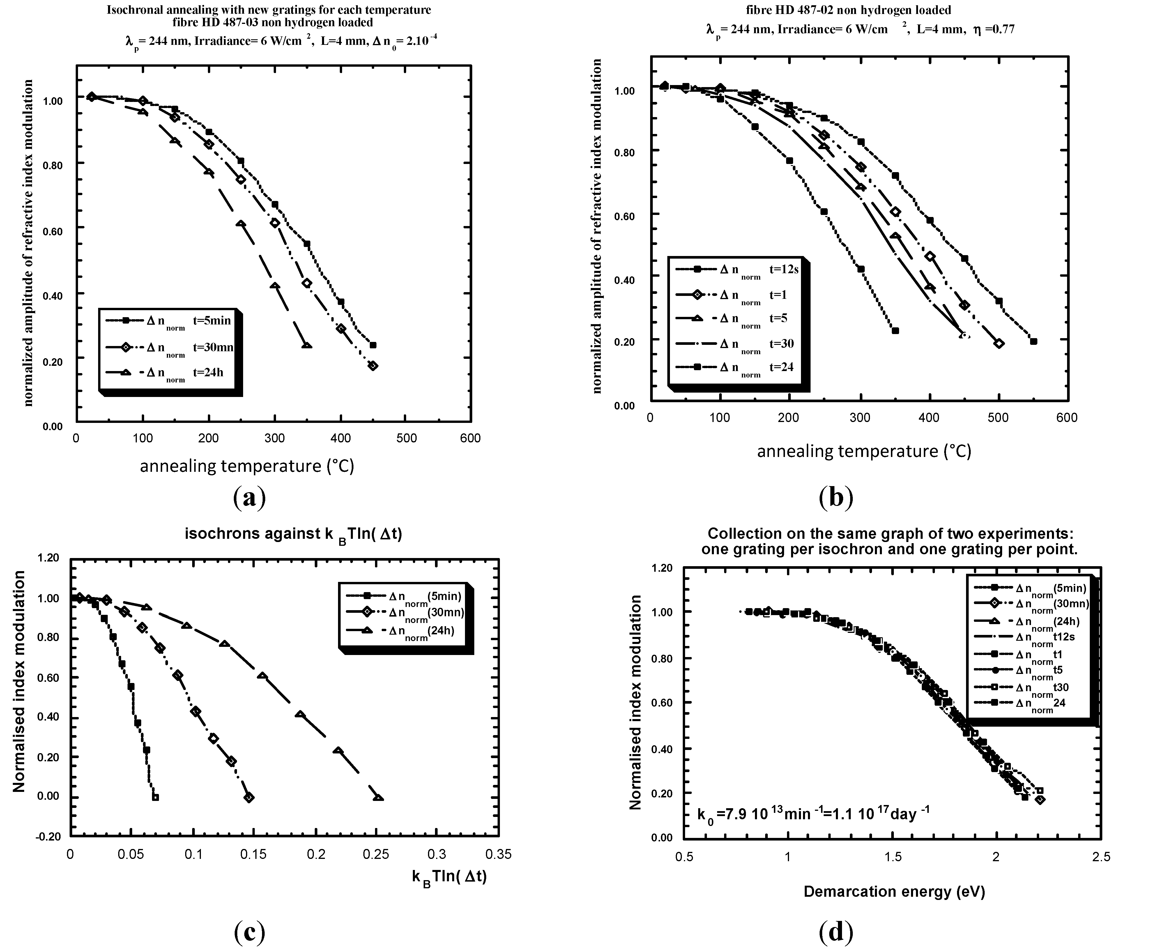
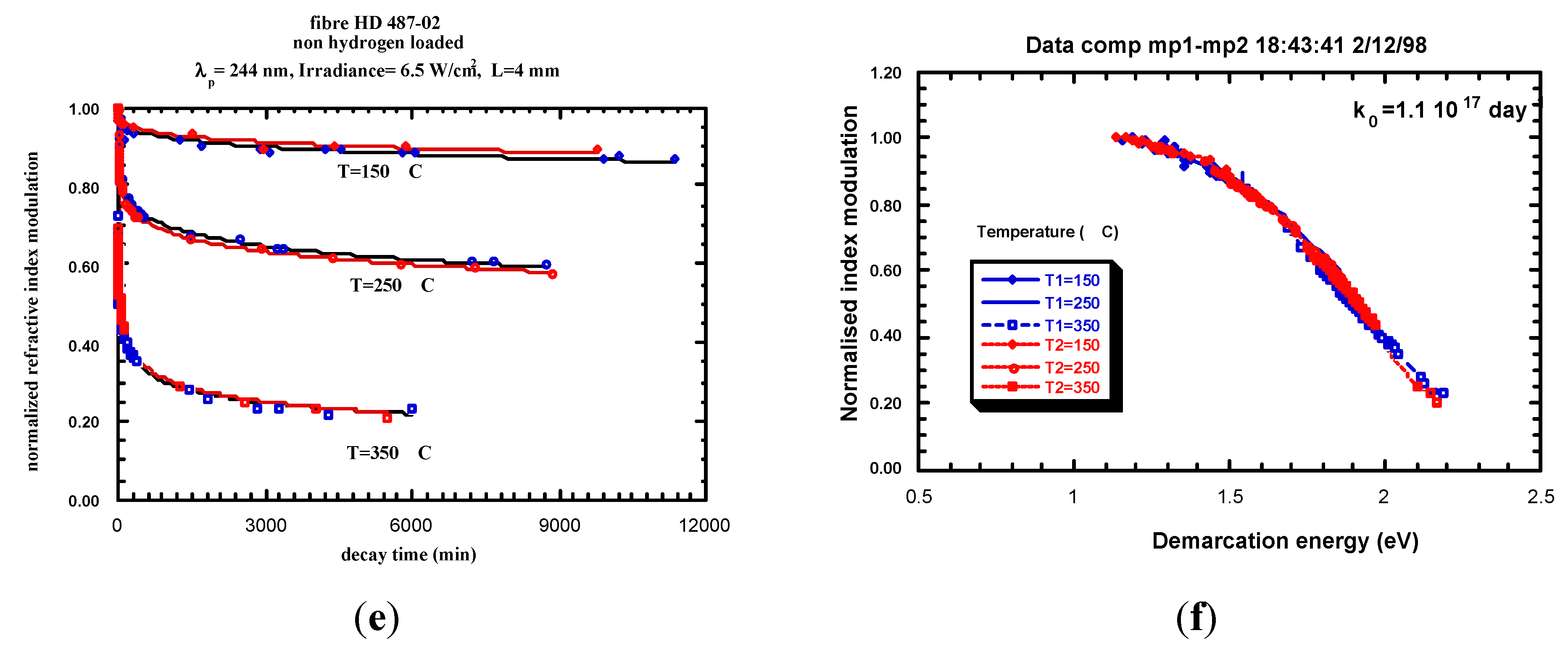
3.1. Distribution Function Determination for the Reverse Reaction

For finding the distribution function when there are no ideas of the shape, one has to follow the same method as in Section 2.2.
(1)
note: d [ B ] d E d = B 0 ( E d ) g ( E d )
(2)
with the assumptions 2.3.1 and 2.3.2 (and even less, i.e., assumption on first order reaction is not necessary).
[ B ] ( t , T ) = 0 ( 1 x ( E E d ) ) B 0 ( E ) g ( E ) d E  with  E d = k B T ln ( k 0 t )
We note that t, T are equivalent ≥ equivalence between isotherms and isochrones.
The main problem is to find k0. This is described here in Figure 29.
(1)
Measurement of several isochrons or isotherms:
(2)
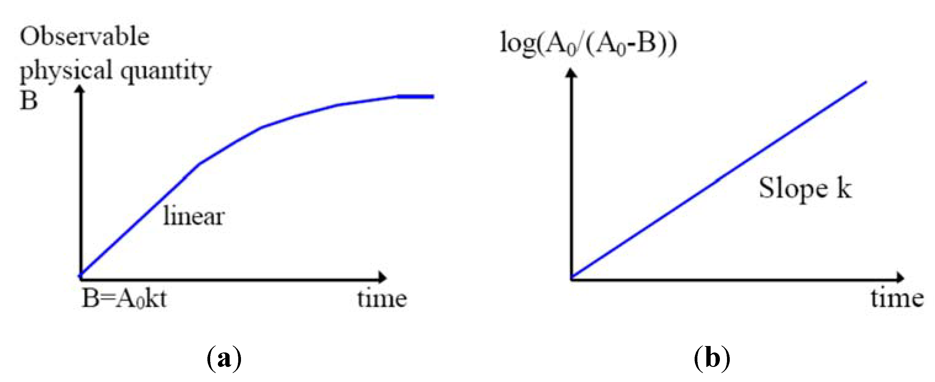
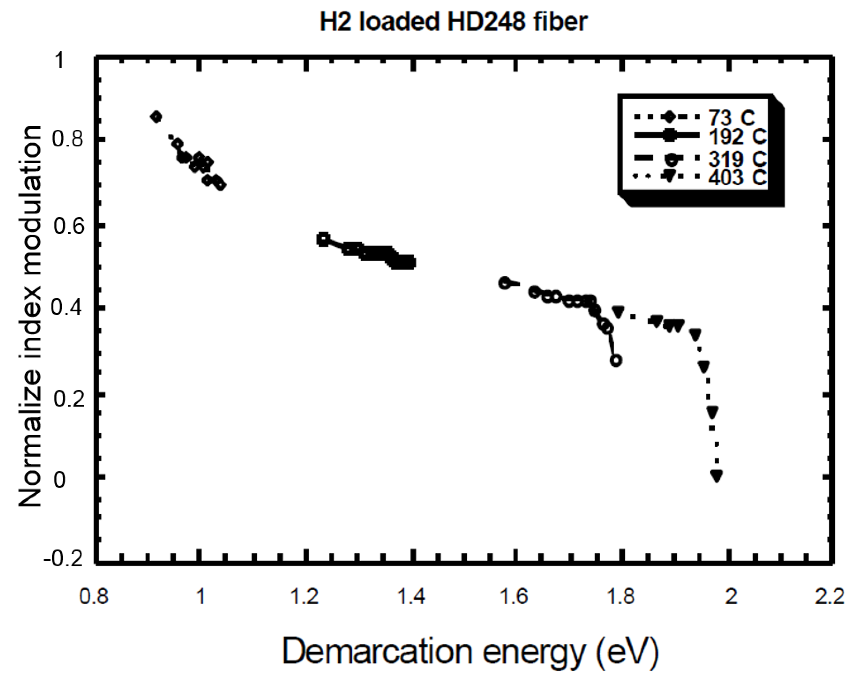
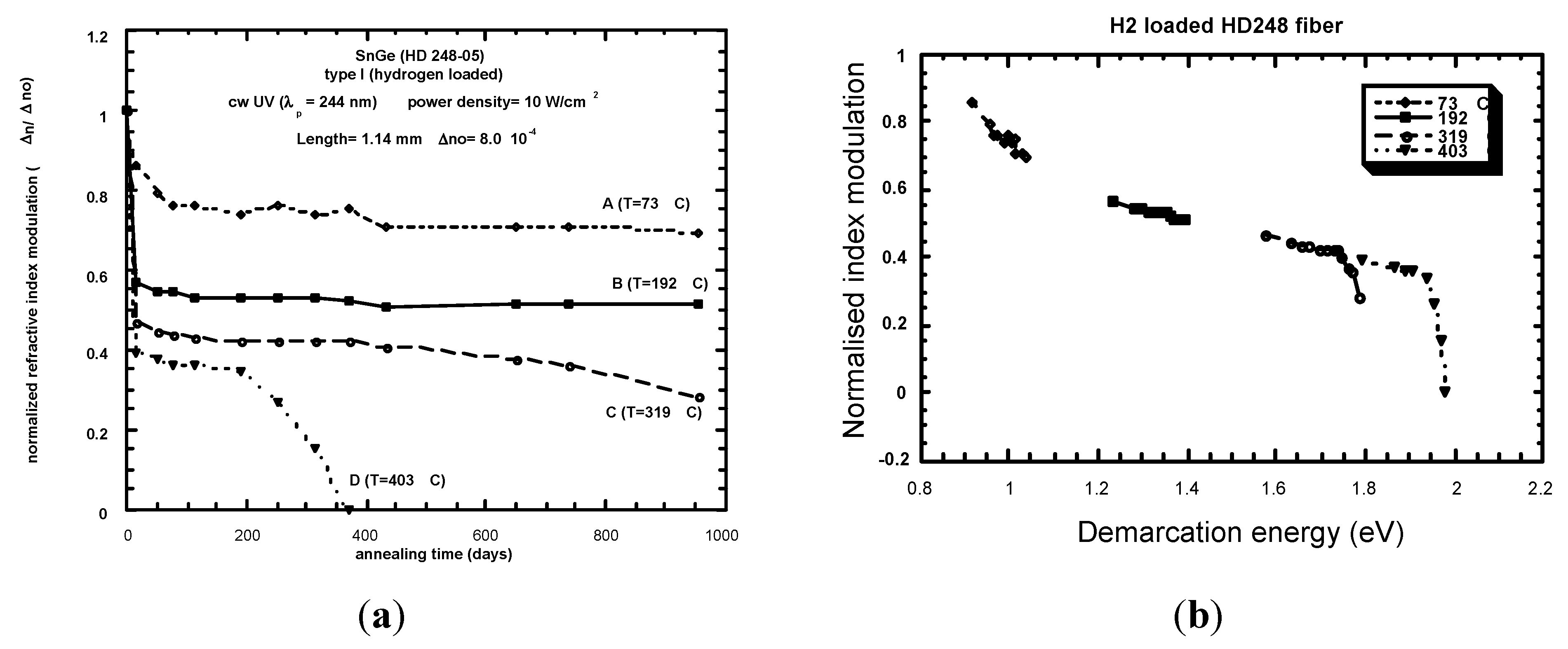
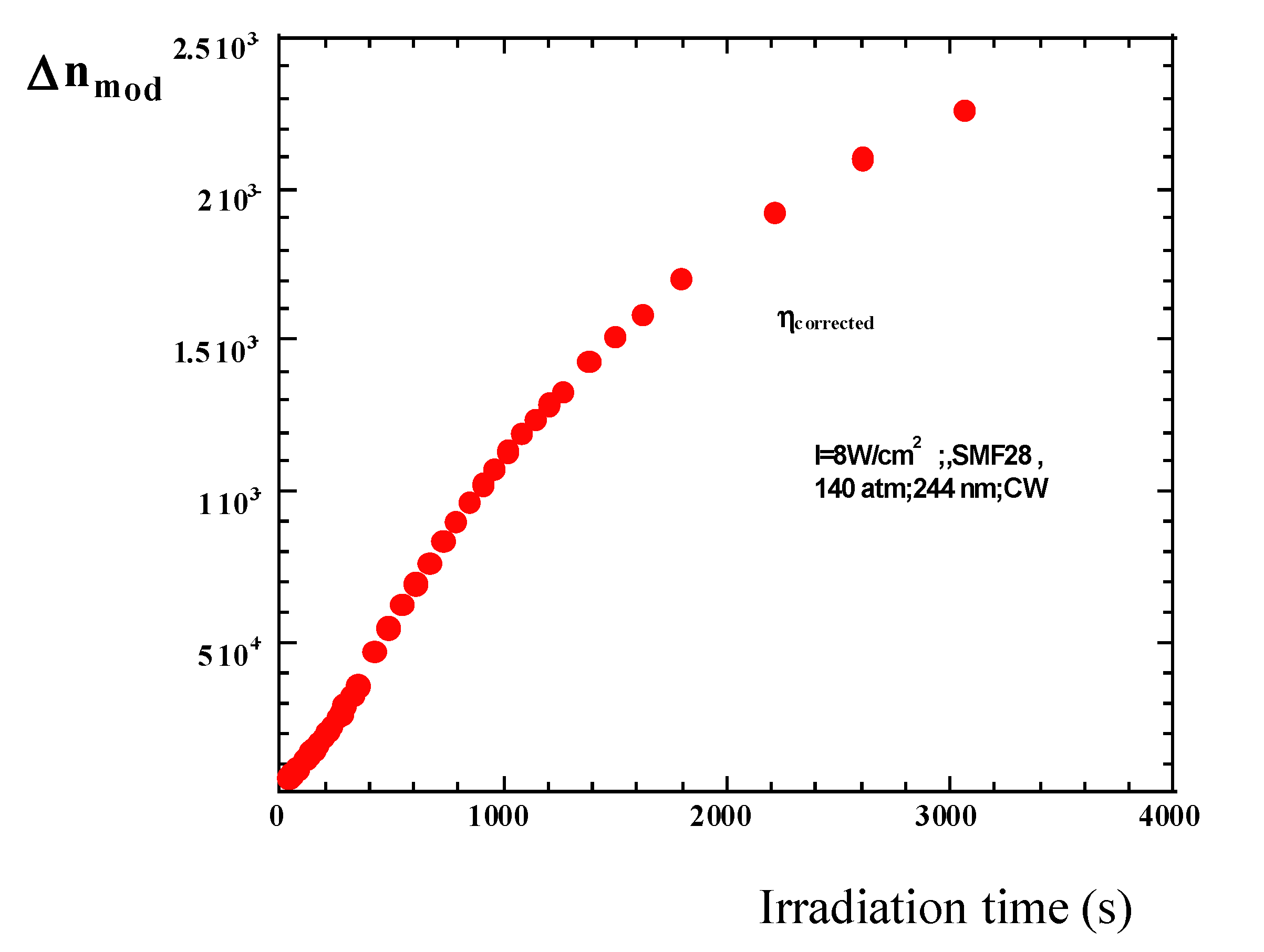
k0 fitting for curve collapsing. We adjust the constant k0 for obtaining the collapse of the curves like in the Figure 29.
(3)
Differentiation of the previous curve. d [ B ] d E d = B 0 ( E d ) g ( E d ) .
Figure 29. Procedure to obtain k0 and g(E).
Fibers 03 00206 g029

3.2. Practice (or application of the theory)
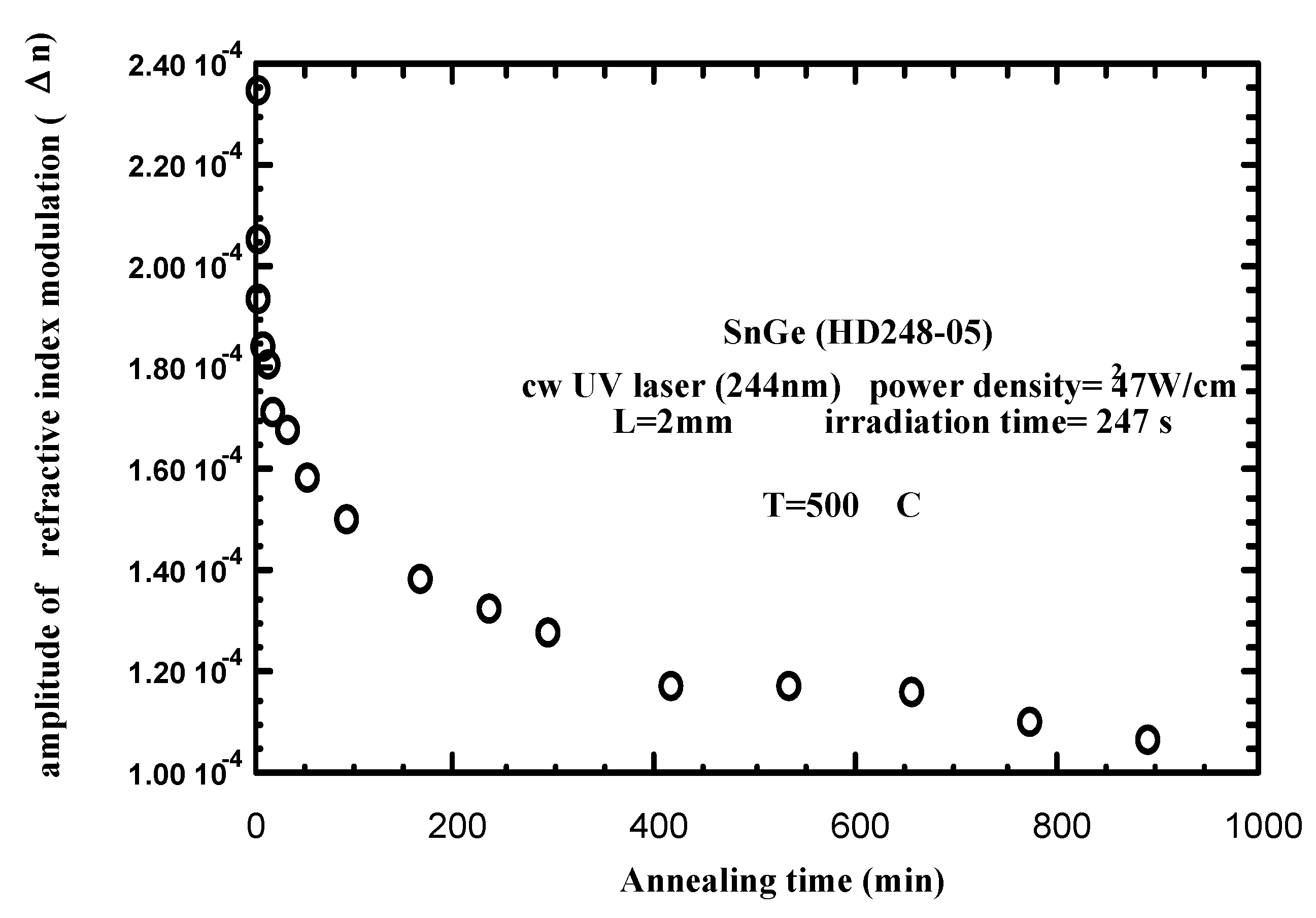
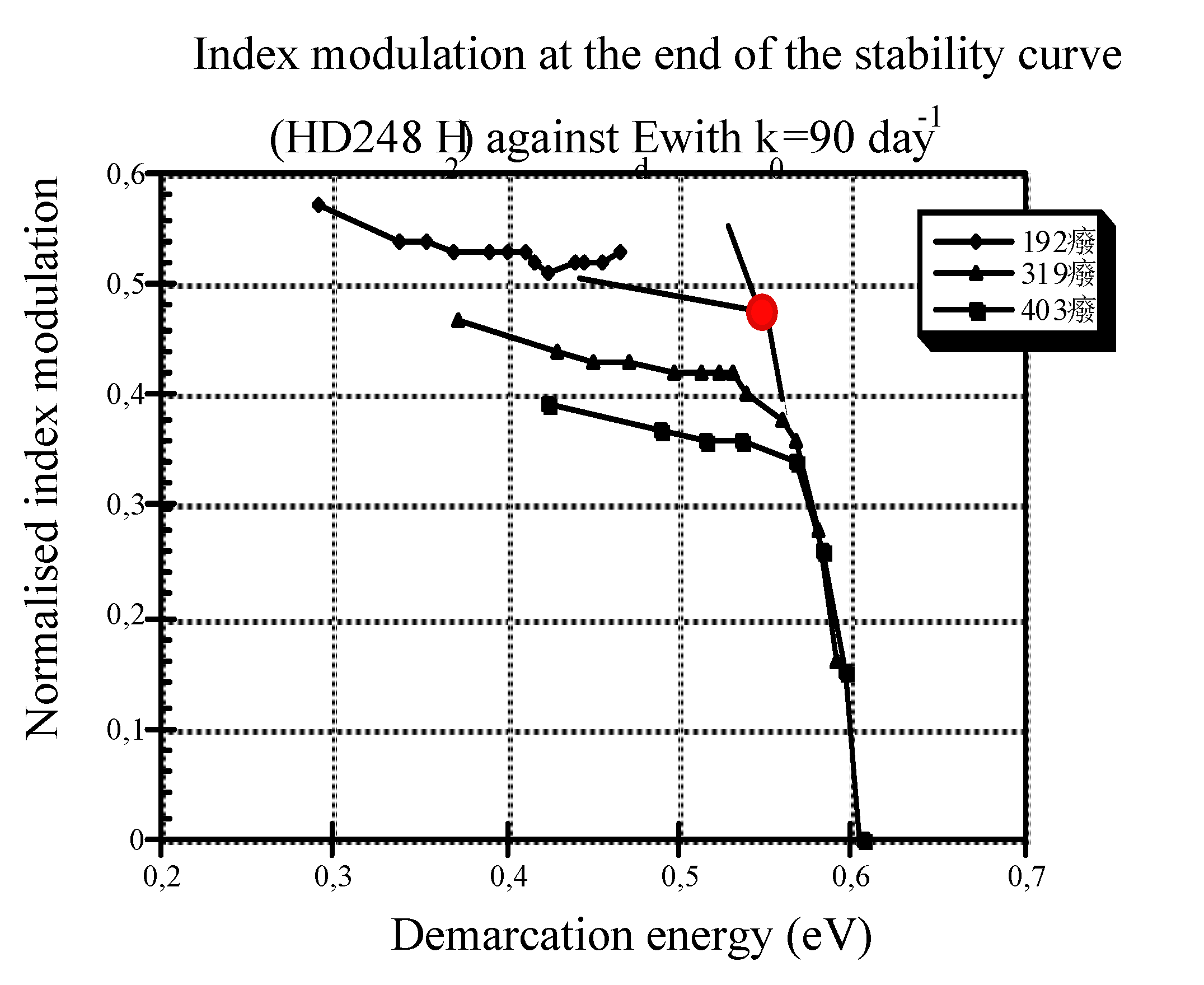
The example we have chosen is the case of Bragg grating, written in a tin doped optical fiber core. Here, we make the assumption that the refractive index change modulation is proportional to point index change (see Section 4). Results are from Razafimahatratra [37]. Five isotherms are available, which we can see in Figure 30 and Figure 31 (79, 194, 299, 386, 500 °C). The last isotherm (Figure 31) is not recorded in the same conditions as the others (index change at the origin is 2.4 × 10⁻⁴ for 500 °C, whereas it is 2 × 10⁻⁴ for the others) but we will see that it is not annoying due to renormalization.
Figure 30. Isotherms from Razafimahatratra, reprinted with permission from [37]. Copyright 2000 University Lille 1.
Fibers 03 00206 g030
Figure 31. Isotherms from Razafimahatratra, reprinted with permission from [37]. Copyright 2000 University Lille 1.
Fibers 03 00206 g031
After plotting against kBTlnt, we obtain Figure 32, which should show parts of parallel curves. We have to align these, looking for the constant k0. This can be done automatically by fitting the polynomial of demarcation energy kBTln(k0t). This has been made in Figure 33, yielding k0 = 0.6 to 2.4 × 10¹² day−1. Here, we can check that it was possible to find a frequency factor, thus that the hypothesis of one order reaction for relaxation is fulfilled. Let us go on to distribution function determination. There are two solutions: one is to differentiate thefitted polynomial and try to fit a known expression, which is possible to find, for instance, in commercial software. Here, it seems realistic that the distribution is a bell shaped function, and, thus, an incomplete sigmoidal function in the case of identical forward and backward pathways (see Section 2.3.4.2). Figure 34 shows the fit in line with the expression below:
Figure 32. Plot of results of Figure 31 against kBTlnt.
Fibers 03 00206 g032
Figure 33. Plot against demarcation energy, an isochron has been added.
Fibers 03 00206 g033
Figure 34. η (the proportion to saturation of the gratings) is found at 72% ± 10%, the rate constant for the stability is 1.2 × 10¹² day−1 ± factor 2, the pre-exponential factor is 2.5 × 10⁻⁴ ± 30% and T0 =2670 ± 200 K.
Fibers 03 00206 g034
[ B ] ( t ) B 1 = 1 ( k 0 t ) T T 0 exp ( E 0 + Δ E k B T 0 ) 1 η η 1 + ( k 0 t ) T T 0 exp ( E 0 + Δ E k B T 0 )
The gratings appear to be non-saturated, written to 72% ± 10% in the sense that the index was not saturated (this has nothing to do with the reflectivity). The pre-exponential factor is 2.5 × 10⁻⁴ ± 30% and T0 = 2670 ± 200 K. As we have seen in Section 3.1, under the validity of a few assumptions, there is a lnt, T equivalence. The plot of an isochron in Figure 33 shows a shift that is explained by Niay et al. [37] by the different temperature of measurements of the reflectivity.

3.3. Stabilization

Since the life function is now available, it is possible that, for a maximum specified temperature of T = 273 + 40 K and 25 years, the grating strength will decrease to 0.974. It is also possible to study the stabilization in order to eventually increase the lifetime of our grating. The principle is based on the distribution of B species stability at various sites. A burning-in process suppresses the less stable sites (see Figure 35). This cannot be achieved with a simple exponential kinetics (SIREPA).
Figure 35. Effect of an annealing on B distribution: annealing will erase the less stable species.
Fibers 03 00206 g035
This widespread method, used for increasing the stability of an FBG (Fiber Bragg Grating) after its inscription, consists in post-annealing the FBG for a time tanneal at a temperature Tanneal > Tuse. A coherent rationale of this method is formulated from the above-mentioned approach: the treatment wipes out the portion of the index change that would normally decay over the lifetime of the device, and keeps only the stable portion of the index change. Notice that this method proves to be effective for enhancing the stability of index changes in either non-hydrogenated or H2-loaded Ge-doped fibers.
As shown in Figure 36, the stabilization (passivation) induced by an annealing can be computed by renormalizing the final value of the index change Δnf after a time tuse at temperature Tuse by the index change Δn1 after burning in process. If we impose that after a given time at a given temperature (let us say 25 years at 40 °C for instance), the lifetime ratio Δnfn1 has to remain within a given range 1 ε < Δ n f Δ n 1 < 1 with ε < 10%, as an example, we obtain the passivation parameters (time ta and temperature Ta). Notice that, in general, we estimate the uncertainty on k0 based on the data uncertainty, then we chose the worst case value and we added an extra safety margin (typically ε < 1% instead of 10%). A thorough analysis is shown in [38].
From practical point of view and as shown in Figure 36, the stabilization (passivation) is usually defined by a passivation ratio, noted as Δn0n1, which is defined by the FBG index modulation Δn1 (or its reflectivity) after a passivation time ta at a given passivation temperature Ta by the FBG index modulation Δn0 (or its reflectivity) before the passivation process. Thus, if the end user imposes that after a given time tuse at a given temperature Tuse (25 years at 45 °C, for instance), the lifetime ratio Δnfn1 has to remain within a given range 1 ε < Δ n f Δ n 1 < 1 with ε < 1% for instance, we determined the related passivation ratio Δn0n1, e.g., 2. This means that the passivated FBG at a chosen passivation temperature Ta (e.g., 220 °C in our study) must be erased of about a factor of two to respect the above-mentioned lifetime criteria (ε < 1% during 25 years at 45 °C). Using the data in Figure 34, here we have, 33 h at 110 °C.
Figure 36. Scheme of the passivation process (also called burn-in process in this figure). Δn0 is the FBG index modulation (or its reflectivity) before the passivation process at the temperature Ta for a given time ta. Δn1 is the FBG index modulation after the passivation process. Δnf is the final value of the index change after its life for a time tuse at a given temperature Tuse.
Fibers 03 00206 g036
Important remark:
If the condition of aging of a system is reliable, the master curve of the passivated system can be deduced from the MC of the passivated system. Then, this new MC can be compared with an experimental one built from the passivated system. This works very well, but some precautions have to be taken when performing the comparison. More details can be found in pages 50–67 in [38]. Important points are as follows:
-
the non-passivated master curve after annealing is truncated and needs to be renormalized.
-
the origin of the time is usually taken from the beginning of the ageing after annealing and, thus, a time shift has to be applied on the previous demarcation energy. This is not negligible in the first 3% of ageing (see page 52 of [38]).

4. Peculiar Properties in the Frame of Assumption Validity (Action of the Reversed Reaction)

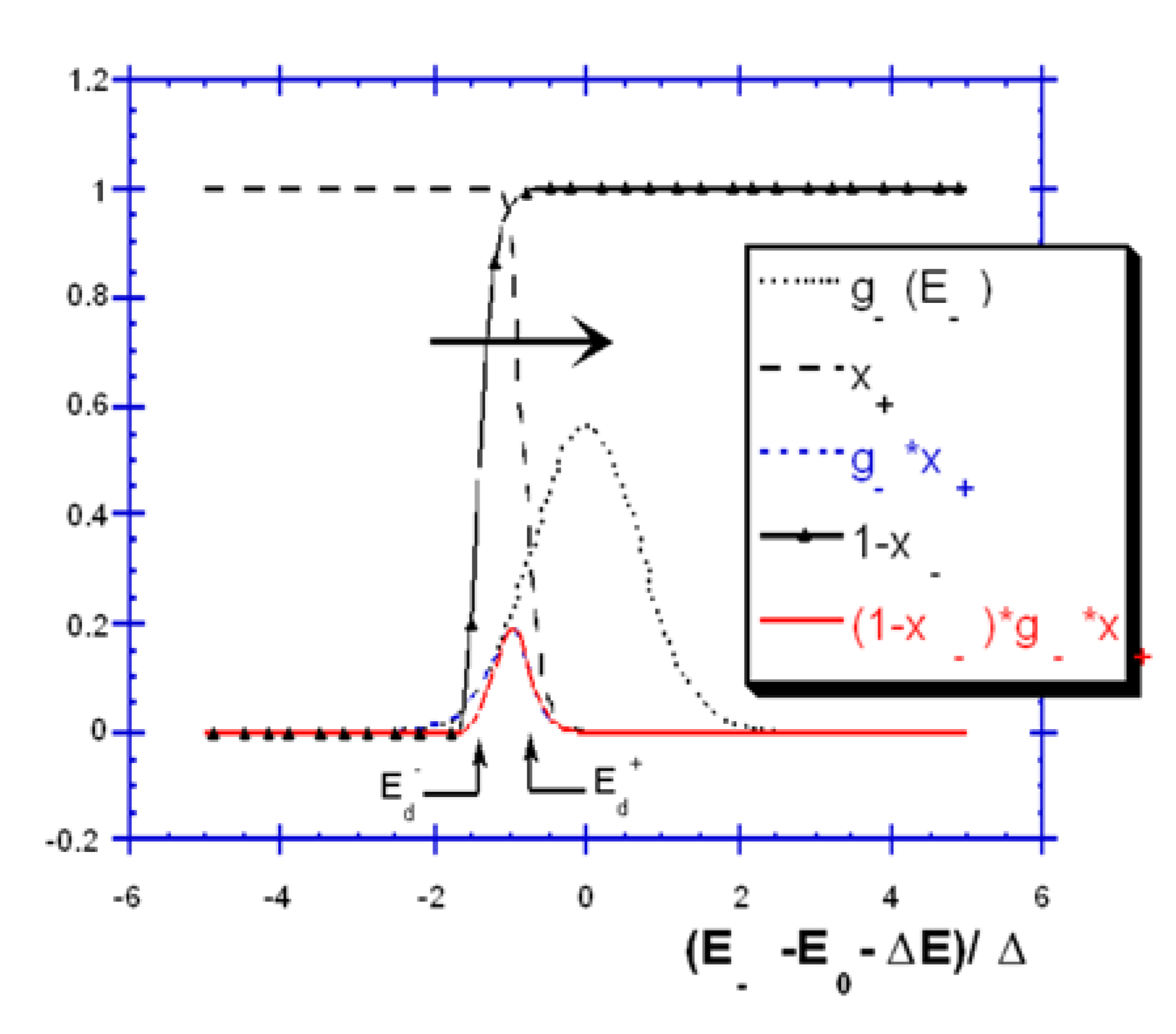
4.1. Writing-Erasure Connection (A⇒B, B⇒A)

We have seen that it is interesting to write at the highest temperature because Ed increases on T and, thus, also the stability (see Section 2.3.4). However, sometimes the reverse reaction (B⇒A) becomes active, introducing a limitation. It cannot be neglected anymore regardless of whether the forward and backward pathways are the same or not.
For high T, equilibrium is developed regardless of if either the g+ or g distributions are dependent or not from each other because the reverse reaction can no longer be neglected.
(1)
Case 1 (same pathways): we will show that the distribution function is cut at large Ed at a more elevated temperature. Stability increases because more stable sites are filled [36] (see Section A below).
(2)
Case 2 (different pathways, two distribution functions): stability increases because less stable sites are removed in the reverse distribution function during writing (Section B below).

4.1.1. Writing in the Case of Reversible Reaction

The equations applicable in the case of reversible kinetics are written below. Now, the degree of advancement x+ will never reach 1, but will remain limited by the rate k + 0 / k T 0 .
A k + k B x / ( E + , t , T ) = k + 0 k T 0 ( 1 exp ( k T t ) ) with  k T 0 ( T ) = k + 0 + k 0 exp ( Δ E k B T )
Using the same procedure as in Section 2.2.3, the integral of B is solved with a new expression for the demarcation energy, including the total rate constant in the E+ scale ( k T 0 ( T ) , E D + = k B T ln ( k T 0 ( T ) t ) (see [36]). Using a distribution from differentiation of a sigmoid, we get the following expression:
[ B ] ( t ) = A 0 k + 0 k T 0 ( k T 0 ( T ) t ) T T 0 exp ( E 0 k B T 0 ) 1 + ( k T 0 ( T ) t ) T T 0 exp ( E 0 k B T 0 ) | α = T T 0 a = exp ( T T 0 ln ( k T 0 ( T ) ) E 0 k B T 0 )
The expression of [ B ] ( t , T ) reveals that power law with the same exponent as in Section 2 is still followed, but the pre-exponential factor is modified. Now, the dependence of the pre-exponential factor a is super-exponential. This is due to the variation of total rate constant with temperature. The growth of index during writing will be faster at a higher temperature, but limited to k 1 0 / k T 0 , which itself decreases with temperature. Thus, there is a compromise. Ed is no more proportional to T and, thus, it is no longer possible to find a k0 with isochronous experiments. Two parameters are necessary k + 0   and   k 0 . The equivalence between lnt and T is broken.
Figure 37 is an example from P. Bernage et al. [4], where we can see that the reverse reaction becomes predominant at high temperature.
Figure 37. Writing kinetics results from Bernage et al., reprinted with permission from [4]. Copyright 1996 University Lille 1.
Fibers 03 00206 g037

4.1.2. Erasure in the Case of Reversible Reaction

In this case, only the backward reaction A k B is active because the forward rate is nulled when light power density is zero. The expression for [ B ] ( t , T ) is the same as in Section 2.3.4 replacing k + 0 with k T 0 in the corresponding expression for stability. Conclusions are, thus, the same as in the previous section, except that the temperature dependence is slightly more complex, as we can see in the formula below:
E D + = k B T ln ( k T 0 T t ) ; E D = k B T ln ( k 0 T t ) ; E E + = Δ E
B 0 ( E + , t w , T w ) = A 0 k + 0 k T 0 [ 1 exp ( k + ( E + , T w ) t w ] ; [ B ] ( t , T ) = 0 B 0 ( E + , t w , T w ) exp ( k ( E , T ) g ( E ) d E
A k B  k = k 0 exp ( E k B T ) ; [ B ] ( t , T ) = A 0 k + 0 k T 0 E d E d + + Δ E g ( E ) d E = 0 k + 0 k T 0 E d Δ E E d + g + ( E + ) d E +

4.1.3. Stability When Forward and Backward Reactions Are Independent

The results in Figure 38 are stability of Bragg gratings, written at different temperature in H2-loaded fibers. They are increasing as the writing temperature increases. The distribution function of the backward reaction is a top hat function since, in this isochronous plot, the curve is linear from ordinate (results above 800 °C are relevant of a second mechanism which is not presented in this paper. The distribution function for the forward reaction is probably a bell shape curve when a power law is detected, or more complex as two successive reactions are noted (see Section 5.3). Forward and backward distributions are independent as stability of gratings written with different strength, but at the same temperature, exhibit the same stability [39]. The expression is similar to the one in Section 2.3.3.
Figure 38. Stability of gratings written with the same Δn0 but at a different temperature.
Fibers 03 00206 g038
During writing at room temperature only reaction A→B is working, the square distribution lies from room T to 800 °C. At a writing temperature of 235 °C, the chemical reaction needs less time to reach the same index change because the writing reaction is thermally activated. On the other hand, the reverse reaction is also thermally activated. This results in a partial bleaching of the species induced by the forward, i.e., the less stable sites. Therefore, the distribution function is “eaten” on the low energy side. As the distribution integral area should remain constant, its magnitude increases.

4.1.4. Writing in the Case of Independent Forward and Backward Reactions

The resolution in this case is not obvious. Let us observe the following equations:
A k 1 + k B x + ( E + , E , T ) = k + k T ( 1 exp ( k T t ) ) with  k T = k + + k
B ( t , T ) = 0 0 g + ( E + ) g ( E ) k + ( E + ) k T ( E + , E ) ( 1 exp ( k T ( E + , E ) ) ) d E + d E
The fact that there is no relation between E+ and E, and that there is E+ and E in kT, renders the double integral unsplitable. As there is no simple solution for solving it, we will not go further in this direction. We can simply note that a limitation appears due to a reversible reaction.

4.2. Isotherm-Isochron Equivalence

Before comparing isochrons and isotherms, it is necessary to be sure that the various measurements have been achieved at the same temperature, room temperature as an example. This means that the grating is quenched at room temperature after annealing at another temperature. This problem has been addressed extensively by Razafimahatratra et al. [40].
A second problem is that the isochrons steps have to be performed correctly, i.e., isochrons steps must be independent. This is achieved under the condition ( δ t k 0 ) Δ T T max < < 1 , where δt is the duration of the annealing step, ΔT is the temperature-step increase, and Tmax is the maximum temperature achieved on the isochrons. In that case, taking a new grating for each isochrons or using the same grating, step-by-step, are equivalent, as is shown in Figure 39a–d.
From the simple theory, Δn = f(Ed), Ed = kBTln(k0t) <=> (lnt, T) equivalence.
Relevant assumptions:
-
the distribution function is not T dependent,
-
only one limiting reaction.
Figure 39. Set of isochrons and isotherm obtained by, reprinted with permission from [40]. Copyright 2000 University Lille 1. (a,b) compare isochrons obtained on the one hand and from one grating for each temperature, and on the other, with one grating by isochrones; (c) is the curve beam obtained after replotting, as mentioned in Section 3.1; (d) is the master curve deduced for the isochrones; (e,f) are isotherm experiments The same master curve is obtained after taking into account the temperature of the measurements.
Fibers 03 00206 g039aFibers 03 00206 g039b
Finally, it is possible to plot all results on the same plot using a demarcation and a suitable k0 quantity, here we have used k0 = 1.1 × 10¹⁷ day−1. Using the same k0 constant, it is also possible to rescale the isotherms and to superimpose isochrons and isotherms. This shows that the simple approach is applicable.
  • Example of Equivalence Breaking
Example 1: non-T dependent distribution against the T-dependent one.
Riant et al. [5]: non-T dependent top hat function:
Δ n Δ n 0 = 1 E d E min E max E min ,  g ( E ) = { 0 , E < E min 1 E max E min , E min < E < E max 0 , E max < E
Baker et al. [41]: T dependent top hat function:
Δ n Δ n 0 = 1 E d E min A k B T , g ( E ) = { 0 , E < E min 1 A k B T , E min < E < E min + A k B T 0 , E min + A k B T < E
These two interpretations can be differentiated by comparing isochrons and isotherms, there is t, T equivalence in the first case, and non-t, −T equivalence in the second case.
Example 2: occurrence of a secondary reaction:
In the chosen experiment, described in Figure 40, refractive index change (RIC) is achieved by a 248 nm pulsed laser after H2 loading at a low T high P. The isothermal measurements of a very long period (three years) have been plotted according to the demarcation energy with a rate constant of 1.4 × 10¹² day−1. The distribution curve, which can be obtained by differentiation of the plotted curve for E < 1.7 eV, is, here, closer to a decreasing exponential. The drops at the end of the plot are relevant of another reaction with a much smaller rate constant (90 day−1) [40]. The figure, in the case of highly Ge-doped fiber core, shows that it is not possible to obtain a complete master curve due to another process occurring at the end of high-temperature treatment. There are two reactions, two Ed's are required, and a simple theory is not applicable (see Section 5.2).
Figure 40. Result from [40]. Copyright 2000 University Lille 1. NICC vs. the demarcation energy.
Fibers 03 00206 g040

4.3. k0 Comparison

We have seen before that it is possible to get a master curve by providing only one parameter, i.e., k0 when suitable assumptions are fulfilled. After obtaining k0 and the master curve, we can compare the different stability functions (Figure 41). It is not necessary for this purpose to have a functional of Ed for performing this comparison, but only the assumption of one active reaction. We can observe that the energies lie in the same range. This is due to a restriction effect of an observable property. The shapes of the curves are different, arising from different distribution functions. k0 values, however, are quite different. The weight effect of vibrating species is not enough for explaining the observed range (as it is usual in solid). It is the probability for a cluster formation, i.e., a “transient complex”. The larger the complex is, the smaller the probability is. Other examples can be found in Chabrerie [42], showing that k0 can eventually depend on the effective trapping cross section with a T2 dependence. In any case, k0 gives information on the B species trapping mechanism.
Figure 41. Shape of the stability function of a normalized index for different experimental conditions.
Fibers 03 00206 g041

5. Beyond Simple Theory

5.1. Higher Order Reaction

This problem has been already mentioned by Primak [29]: A k 2 B , k = k 0 exp ( E k B T ) d x d t = k ( E ) x ( E , t ) 2 x ( E , t ) = 1 1 + 1 B 0 t k 0 exp ( E k B T ) , defining Ed with x(E, t) = 1/2, we can compute [ B ] ( t , T ) if B0 does not depend on E in considering x ( E , t ) = 1 1 + exp ( E E d k B T ) as a rapidly varying function of E.
The [ B ] ( t , T ) = B 0 0 x ( E , t ) g ( E ) d E and [ B ] ( E d ) = B 0 E d g ( E ) d E as for first order, but with E d = k B T ln ( B 0 k 0 T ) . The reaction properties are in Ed, and the disorder in g(E), as before. However, Ed depends on B0, i.e., on the grating strength. The main conclusion is that stability, here, depends on the grating strength, even if forward and backward reactions are independent.

5.2. Two Parallel Reactions

Below are experimental results from Razafimhatratra et al. [40] in the case of H2-loaded fiber (Figure 42). A first k0 can be found collapsing the curve at low t and low T (Figure 43). These master curves have been obtained with a rate constant equal to 1.4 × 10¹² day−1. Another k0 can be obtained when collapsing curves at large time or high temperature.
Figure 42. Results from [40], Copyright 2000 University Lille 1. The second master curve for large t and T. Theory of serial reactions. (a) Isothermal annealing curves; (b) Master curve collapsing.
Fibers 03 00206 g042
Figure 43. Corresponding master curve for low t and low T.
Fibers 03 00206 g043
The theory is as follows:
A 1 k 1 A 2 k 2 B d η d t = ( k 1 ( E 1 ) + k 2 ( E 2 ) ) η   η ( E 1 , E 2 , t ) = exp [ ( k 1 ( E 1 ) + k 2 ( E 2 ) ) t ]
   [ B ] ( t ) B 0 = 0 0 exp [ ( k 1 ( E 1 ) + k 2 ( E 2 ) ) t ] g ( E 1 ) g ( E 2 ) d E 1 d E 2
   [ B ] ( t ) B 0 = 0 exp [ k 1 ( E 1 ) t ] g ( E 1 ) d E 1 0 exp [ k 2 ( E 2 ) t ] g ( E 2 ) d E 2
[ B ] ( t ) B 0 = E d , 1 = k B T ln ( k 0 , 1 t ) g ( E 1 ) d E 1 . E d , 2 = k B T ln ( k 0 , 2 t ) g ( E 2 ) d E 2
E d , 1 = k B T ln ( k 1 0 t ) ; E d , 2 = k B T ln ( k 2 0 t )
We note that isotherms and isochrons are, again, no longer equivalent. Let us illustrate the complex behavior of B. We have chosen the constant rate k0,2 as smaller than k0,1. We note that f(Ed,1) and f(Ed,2) are different for a given t, T couple. Ed,1 and Ed,2 do not have the same value (Figure 44a).
Figure 44. (a) Due to different k0, the rate of evolution along reaction 1 or 2 are not the same; (b) Isothermal description. The dashed line shows the evolution of the erasure; (c) Isochronal description. Since the shift of the master curves increases as T increases, the cross point can be not detectable.
Fibers 03 00206 g044
In an lnt plot, the stability curves are shifted from each other (Figure 44b). The fastest reactions are predominant (curve 1) and we almost only see curve 1 behavior in the physical quantity. For a large T, the second behavior appears. At a larger T, curve 1 is shifted more on the left and curve 1 behavior is even more predominant in the behavior of the final physical quantity (Figure 44b). At a large t, curve 2 behavior appears but for a smaller contribution.
Along the isochronal curves in Figure 44c, the temperature changes and the shift between curve 1 and 2 are increased in such a way that process 1 may have erased grating before process 2 appears. This may lead to an error on isothermal lifetime estimate.

5.3. Serial Reactions

Examples of serial reactions can be found in different fields, such as quasi elastic neutron scattering in PVC [43] or E′ center production under X-ray in SiO2 [44], but we will stay in our field, considering the index change during writing after H2 loading of the glass. In this case, a sigmoidal curve is recorded according to the fluence (Figure 45, which is a linear-linear plot, shows a curve with an inflexion point, which is the indication of the occurrence of two serial reactions [45]). Moreover, in this example, the end of the curve reveals a non-exponential behavior.
Figure 45. Index change in H2-loaded SMF28 (Corning) during writing with a CW 244 nm laser, reprinted with permission from [45]. Copyright 2001 University Lille 1.
Fibers 03 00206 g045
  • Theory of Serial Reactions
We consider the two successive reactions, A k 1 B k 2 C . C is supposed to give rise to significant refractive index change. Note that, if one considers that A and B species are contributing to the refractive index change, it is then necessary to take them into account, but this does not cause any difficulties after solving the serial equation.
The solution of this equation, taking into account that the initial content is A0, leads to the following expression for the advancement degree: η = C/A0
η = 1 k 2 k 1 { k 2 [ 1 exp ( k 1 t ) ] k 1 [ 1 exp ( k 2 t ] }
We can consider that the first and the second activation energy barriers are thermally activated. Other cases will then be easily deduced. Thus, we have k 1 = k 01 exp ( E 1 k B T ) and k 2 = k 02 exp ( E 2 k B T ) .
More symmetrically, the above equation can be rewritten as follows, isolating the energy term into the accolade:
η = k 1 k 2 k 2 k 1 { [ 1 exp ( k 1 t ) ] k 1 [ 1 exp ( k 2 t ] k 2 }
We have to define one demarcation energy (because there is only one reaction, but in two steps) as usual, calculating the second derivative of η according to E1 for other fixed quantities (t, T, E2). As the η function is symmetric according to the first reaction and the second reaction, the demarcation energy found by derivation, according to one, will also be the demarcation energy for the second one. Nevertheless, if we do this, the computation is heavy and does not lead to a simple expression. In fact, it is more efficient to study the η function behavior and find an approximation. For this purpose, we will change the variable in order to suppress the time as we perform for more simple cases. This new variable will be an incomplete demarcation energy Ed, which the function study will allow completing. Thus, as there should be symmetry between the two steps of the reaction, we suppose E d = k B T ln ( 2 k 01 k 02 k 01 + k 02 t ) , in other words, the smaller pre-exponential coefficient will dominate in the demarcation energy. Then, we can write exp [ t k 0 i exp ( E i k B T ) ] = exp [ exp ( E i k B T + ln ( k 0 i ) + E d k B T ln ( 2 k 01 k 02 k 01 + k 02 ) ) ] .
Finally, by setting x = E d k B T ln ( 2 k 01 k 02 k 01 + k 02 ) , x i = E i k B T + ln ( k 0 i ) , we obtain the following expression for η:
η ( x , x 1 , x 2 ) = exp ( x 1 + x 2 ) exp ( x 2 ) exp ( x 1 ) [ 1 exp ( ( exp ( x 1 + x ) ) exp ( x 1 ) 1 exp ( ( exp ( x 2 + x ) ) exp ( x 2 ) ]
When this function is plotted for a series of x1 and x2, separated by more than 2.3 (a factor 10 on the rate constants), the expression for η ( x , x 1 , x 2 ) is the same as 1 exp ( ( exp ( x + inf ( x 1 , x 2 ) ) .
Solving [ C ] ( t , T ) = A 0 + + η ( E 1 , E 2 , t , T ) g 1 ( E 1 ) g 2 ( E 2 ) d E 1 d E 2 , we will get one or the other of the two distributions, according to the relative magnitude of the k0’s and the relative position of the distributions along the abscise.

5.4. Narrow and Steep Distribution Function

The approximation of demarcation energy is based on the condition that the distribution function varies slower than x(E, t, T) (see Section 2.2). On the contrary, it is no longer valid, especially as it is not directly applicable for a Dirac distribution function (SIREPA for single reaction pathway). However, it is possible to show that the approach can be extended. This simply needs to consider an experimental distribution function convoluted by the derivative of the advancement degree as described in Figure 46. Here is the demonstration:
(1)  if we look for the experimental distribution by differentiation of B versus the demarcation energy in considering that it is possible to write X(E, t, T) = X(EEd), we get B = 0 g ( E ) X ( E E d ) d E . Then, we get the following: d B d E d = 0 g ( E ) d [ X ( E E d ) ] d E d d E = 0 g ( E ) d X d E ) E E d d E = [ g ( d X d E ) ] E d = g ˜ ( E d )
The experimental distribution is the theoretical distribution broadened by dX/dE (* means the convolution operator):
g ˜ ( E ) experimental distribution  function = g theoretical distribution function ( d X d E ) experimental distribution is the theoretical one broadened by  dX d E w i d t h = 2 k B T
where X ( E 0 , E d ) = 1 exp ( exp ( E d E 0 k B T ) ) .
0 d X d E d ( E E d ) δ ( E E 0 ) d E = d X d E ( E 0 E d )
Figure 46. Derivative of the reaction advancement degree. (a) The two terms involved in the convolution; (b) the experimental distribution.
Fibers 03 00206 g046
In particular, the Dirac function for a simple exponential will appear as a narrow bell shape curve with a width of 2kBT.
(2)  the inverse problem (to find the analytical function for B): If we consider [ g ( d X d E ) ] E d = g ˜ ( E ) and use the cutting method for computing the B integral, i.e., [ B ] ( E d ( t , T ) , T ) = 0 E d ( t , T ) g ˜ ( E , T ) d E . Are we going to find this following expression? [ B ] ( t , T ) = 0 g ( E ) x ( E , t , T ) d E .
In fact, we get the following:
B ( E d ) = 0 E d g ˜ ( E ) d E = 0 g ( E ) X ( E E d ) d E 0 g ( E ) X ( E ) d E 0 if the distribution does  not touch zero energy.
In conclusion, the VAREPA approach can be applied to any distribution performing at the end of a deconvolution. For instance, in the case of a square distribution (Figure 47), such as when the low Ge-doped fiber is hydrogen loaded, the edge of the distribution will be smoothed, giving rise at the beginning of the reaction to a simple exponential behavior on time.
Figure 47. Effective distribution function.
Fibers 03 00206 g047

5.5. Distributed Non-Activated Kinetics (Photochromism, Luminescence)

5.5.1. “Writing like”

The equation of excitation is the following one: d A * d t = ε ( ) A P , where P is the intensity. We can note that, if ε(hν) (the absorption cross section) is varying rapidly on hν (edge absorption), we can use the VAREPA approach to compute the excited state concentration, excited under white light.
A a f A * , d A * d t = ε ( a ) A P , with  ε(hν a ) = ε 0 exp ( a Δ )
More generally, we have d x d t = k ( 1 x ) , x = 1 exp ( k t ) , k = k ( E / E 0 ( ζ ) ) , where E is the distributed variable with g(E) as the distributed function, ξ is the variable related to the energy source, and E0 is a function of this variable with the same dimension as the distributed variable.
We get:
[ A * ] ( t , ζ ) = A 0 0 E d g ( E ) d E , E d  defined  as  2 x E 2 ) t , ζ ( E = E d ) = 0 E d ( t , ζ )
It is worth noting that the distribution is characterized by the shape of the distribution and a width that we can find, again fixing a value of ξ as ξ0.

5.5.2. Erasure

The erasure corresponds to luminescence. The intensity of this is proportional to d A * d t . If the stability of the luminescence site is distributed, the lifetime will increase on time. In that case, we have:
d A * d t = k . A * ,  k = k 0 exp ( E k B T )
this is the same as in Section 2.3 and the analysis procedure is the same.

6. Real Analysis of Bragg Grating Writing and Stability

In analysis of the refractive index changes, photo-induced in fiber Bragg gratings, we have to pay attention that we work on index modulation and average index changes, but not on point one. However, all theories developed above are for point index change. The difference between these two quantities is a Fourier transform along z, i.e., along Power density fluctuations. To make the link between them, it is, therefore, necessary to know the relationship between k0t and P. Is k0 proportional to P or to P2?
The determination of this k0 dependence has been recently reviewed in Reference [46]. Of course, non-linear dependence on P combined with the non-linear behavior on k0t will lead to a distortion of the interference pattern and to bandwidth broadening. However, this is not the only detrimental effect. Recalling the conclusion of Section 2.3.4, the stability of inter-fringe will be smaller than the one at the maximum of the bright UV fringes. Therefore, during a burn-in process, non-H2 loading fibers made by a pulsed laser (for instance) can exhibit a broadening.

7. Practical Formalism to Describe Generalized Thermally Activated Processes

It is worth noting that a general approach, applicable to any activation energy process analyzed by any experimental measurement (isothermal, isochronous or tempering), has been published by Miller et al. [32]. These authors demonstrate a numerical solving of the generalized equation in which k0, T, or the energy reference can be time dependent. Again, they use a cutting energy, which is defined by 2 x E t | E = E d = 0 .
Specifically, for tempering, the demarcation energy is defined by an expression quite different than for isothermal experiments.
E d k B T + ln ( E d k B T + 2 ) = ln ( k 0 c k B T )
where c is defined by T ( t ) = t c k B + T 0 [42].

8. Conclusions

We have shown a development of a framework for modeling the thermally activated processes, either for creating or erasing species, such as the ones involved in UV-induced refractive index changes [46], based on distributed activation energy of a physico-chemical reaction. From experimental measurements (isochrons and isotherms), this framework allows to find the distribution function, providing only a constant, which can be determined by a simple variable change when a few assumptions are verified. From this distribution, it is possible to know the complete time behavior and to determine the annealing conditions for extending lifetimes.
This approach can be used for other physical quantities, e.g., photodarkening, stress relaxation, and luminescence decay. Finally, let us mention that the framework developed here for the time evolution of an activated energy process can be used for analyzing the frequency behavior of similar system. For instance, Perlmutter et al. [47] describe quasi-elastic light-scattering spectrum analysis in the range of 0.1 to 100 MHz, in term of energy barrier distribution of sites similar to a Poisson distribution. The demarcation energy analog here is kTln(k0/ω).

Acknowledgments

We are very grateful to Pierre Niay and Marc Douay for many discussions and the availability of their measurements. I thank also Christian Chabrerie and Sylvain Costes for their important thesis.

Author Contributions

Bertrand Poumellec interprets the experimental data and wrote the paper. Matthieu Lancry and Bertrand Poumellec conceived, devised and helped carry out the experiments, edited the paper and suggested some new directions.

Conflicts of Interest

The authors declare no conflict of interest.

References

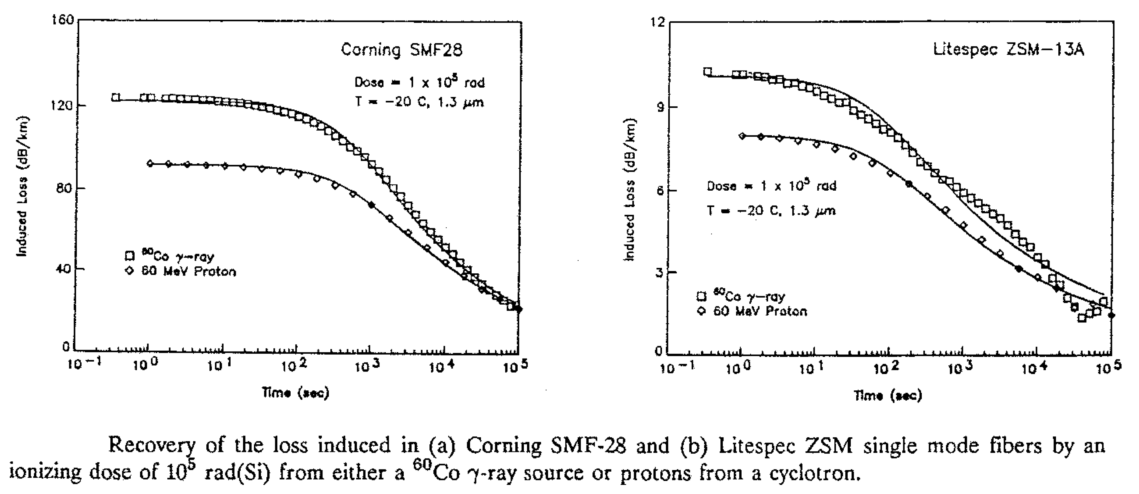
  1. Erdogan, T.; Mizrahi, V.; Lemaire, P.J.; Monroe, D. Decay of ultraviolet-induced fiber Bragg gratings. J. Appl. Phys. 1994, 76, 73–80. [Google Scholar] [CrossRef]
  2. Ishikawa, S.; Inoue, A.I.; Harumoto, M. Adequate aging condition for fiber Bragg grating based on simple power law model. In Optical Fiber Communication Conference and Exhibit, 1998, OFC '98. San Jose, CA, USA, 22–27 February 1998.
  3. Richert, R.; Blumen, A. Disorder Effects on Relaxational Processes; Springer Verlag: New York, NY, USA, 1994. [Google Scholar]
  4. Bernage, P.; Taunay, T.; Leconte, B.; Douay, M.; Niay, P.; Bayon, J.F.; Poignant, H.; Herlemont, H.; Legrand, J.; Poumellec, B.; et al. Inscription Kinetics and Thermal Stability of Bragg Gratings Written within Heated Fibers. In Proceedings of the Doped Fiber Devices and systems II, Denver, CO, USA, 20 November 1996.
  5. Riant, I.; Poumellec, B. Thermal decay of gratings written in hydrogen-loaded germanosilicate fibers. Electron. Lett. 1998, 34, 1603–1604. [Google Scholar] [CrossRef]
  6. Lancry, M.; Poumellec, B.; Costes, S.; Magné, J. Reliable Lifetime Prediction for Passivated Fiber Bragg Gratings for Telecommunication Applications. Fibers 2014, 2, 92–107. [Google Scholar] [CrossRef]
  7. Xie, W.X.; Niay, P.; Bernage, P.; Douay, M.; Taunay, T.; Bayon, J.F.; Delevaque, E.; Monnerie, M. Photoinscription of Bragg gratings within preform plates of high NA germanosilicate fibers: Searching for an experimental evidence of type IIA photosensitivity in preform plates. Opt. Commun. 1996, 124, 295–300. [Google Scholar] [CrossRef]
  8. Poumellec, B.; Niay, P.; Douay, M.; Bayon, J.F. The UV induced refractive index grating in Ge-SiO2 preforms: Additional CW experiments and the macroscopic origin of the change in index. J. Phys. D Appl. Phys. 1996, 29, 1842–1856. [Google Scholar] [CrossRef]
  9. Fiori, C.; Devine, R.A.B. Ultraviolet irradiation induced compaction and photoetching in amorphous, thermal SiO2. MRS Proc. 1986, 61, 187–195. [Google Scholar] [CrossRef]
  10. Primak, W.; Kampwirth, R. The radiation compaction of vitreous silica. J. Appl. Phys. 1968, 39, 5651–5658. [Google Scholar] [CrossRef]
  11. Allan, C.D.; Smith, C.; Borelli, N.F.; Seward, T.P., III. 193-nm excimer laser induced densification of fused silica. Opt. Lett. 1996, 21, 1960–1962. [Google Scholar] [CrossRef] [PubMed]
  12. Lemaire, P.J. Reliability of optical fibers exposed to hydrogen: Prediction of long-term loss increases. Opt. Eng. 1991, 30, 780–789. [Google Scholar] [CrossRef]
  13. Marcerou, J.F.; Février, H.; Gabla, P.M.; Augé, J. Sensitivity of erbium-doped fibers to hydrogen: Implications for long-term system performance. In Proceedings of the Optical Fiber Communication’94, San Jose, CA, USA, 20–25 February 1994.
  14. Beales, K.J.; Cooper, K.J.; Rush, J.D. Increased attenuation in optical fibers caused by diffusion of molecular hydrogen at room temperature. Electron. Lett. 1983, 19, 917–919. [Google Scholar] [CrossRef]
  15. Smith, C.L. A theory of transient creep in metals. Proc. Phys. Soc. 1948, 61, 201–205. [Google Scholar] [CrossRef]
  16. Poirier, M.; Thibault, S.; Lauzon, J.; Ouellette, F. Dynamics and orientational behaviour of U.V. induced luminescence bleaching in Ge-doped silica optical fiber. Opt. Lett. 1993, 18, 870–872. [Google Scholar] [CrossRef] [PubMed]
  17. Erdogan, T.; Mizrahi, V.; Lemaire, P.J.; Monroe, D. Decay of U.V.-induced fiber Bragg gratings. In Proceedings of the Optical Fiber Communication’94, San Jose, CA, USA, 20–25 February 1994.
  18. Kyung, J.H.; Lawandy, N.M. Direct observation of the effective χ(2) grating in bulk glasses encoded for second-harmonic generation. Opt. Lett. 1996, 21, 632–634. [Google Scholar] [CrossRef] [PubMed]
  19. Friebele, E.J.; Gingerich, M.E.; Griscom, D.L. Survivability of optical fibers in space. In Proceedings of the Optical Materials Reliability and Testing, Boston, MA, USA, country, 8 September 1992.
  20. Deparis, O.; Griscom, D.L.; Mégret, P.; Decréton, M.; Blondel, M. Influence of the cladding thickness on the evolution of the NbOHC band in optical fibers exposed to gamma radiations. J. Non Cryst. Solids 1996, 216, 124–128. [Google Scholar] [CrossRef]
  21. Rodriguez, V.D.; Rodriguez-Mendoza, U.R.; Martin, I.R.; Lavin, V.; Nunez, P. Site distribution in Cr3+ and Cr3+-Tm3+ doped alkaline silicate glasses. In Proceedings of the SiO2 and Advanced Dielectrics, L’Aquila, Italy, 15–17 June 1997.
  22. Monroe, D.; Kastner, M.A. Exactly exponential band tail in a glasssy semiconductor. Phys. Rev. B 1986, 33, 8881–8884. [Google Scholar] [CrossRef]
  23. Kroide, M. Apparent viscosity and relaxation mechanism of glasses below glass transition temperature. Phys. Chem. Glasses 1997, 38, 83–86. [Google Scholar]
  24. Phillips, J.C. Kohlrausch relaxation and glass transitions in experiment and in molecular dynamics simulations. J. Non Cryst. Solids 1995, 182, 155–161. [Google Scholar] [CrossRef]
  25. Mohanna, Y.; Saugrain, J.-M.; Rousseau, J.-C.; Ledoux, P. Relaxation of internal stresses in optical fibers. J. Lightwave Technol. 1990, 8, 1799–1802. [Google Scholar] [CrossRef]
  26. Lemaire, P.J.; Tomita, A. Behavior of single mode MCVD fibers exposed to hydrogen. In Proceedings of the European Conference on Optical Communications, Stuttgart, Germany, 3–6 September 1984.
  27. Kohlrausch, R. Ueber das Dellmann’sche Elektrometer. Ann. Phys. 1847, 72, 353–405. (In German) [Google Scholar] [CrossRef]
  28. Vand, V. A theory of the irreversible electrical resistance changes of metallic films evaporated in vacuum. Proc. Phys. Soc. Lond. 1943, A55, 222–246. [Google Scholar] [CrossRef]
  29. Primak, W. Kinetics of Processes distributed in activation energy. Phys. Rev. B 1955, 100, 1677–1689. [Google Scholar] [CrossRef]
  30. Primak, W. Large temperature range annealing. J. Appl. Phys. 1960, 31, 1524–1533. [Google Scholar] [CrossRef]
  31. Orenstein, J.; Kastner, M. Photocurrent transient spectroscopy: Measurement of the density of localized states in a-AS2Se3. Phys. Rev. Lett. 1981, 46, 1421–1424. [Google Scholar] [CrossRef]
  32. Miller, S.L.; McWhorter, P.J.; Miller, W.M.; Dressendorfer, P.V. A practical predictive formalism to describe generalised activated physical processes. J. Appl. Phys. 1991, 70, 4555–4568. [Google Scholar] [CrossRef]
  33. Lemaire, P.J.; Monroe, D.P.; Watson, H.A. Hydrogen-induced-loss increases in erbium-doped amplifier fibers: Revised predictions. In Proceedings of the Optical Fiber Communication’94, San Jose, CA, USA, 20–25 February 1994.
  34. Vandenbrink, J.P. Master stress relaxation function of silica glasses. J. Non Cryst. Solids 1996, 196, 210–215. [Google Scholar] [CrossRef]
  35. Kannan, S.; Lemaire, P.J.; Guo, J.; LuValle, M.J. Reliability predictions on fiber gratings through alternate methods. In Proceedings of the Bragg Gratings Photosensitivity, and Poling in Glass Fibers and Waveguides: Applications and Fundamentals, Williamsburg, VA, USA, 26–28 October 1997.
  36. Poumellec, B. Links between writing and erasure (or stability) of Bragg gratings in disordered media. J. Non Cryst. Solids 1998, 239, 108–115. [Google Scholar] [CrossRef]
  37. Razafimahatratra, D.; Thesis, P. Etude de la Stabilité de la Variation D’indice de Réfraction Photoinduite par Insolation Laser Dans les Guides D’onde Optiques Germanosilicates. PhD Thesis, University of Sciences and Technologies of Lille, Lille, France, 2000. [Google Scholar]
  38. Costes, S. Extension de L’approche par la Courbe Maîtresse de la Prédiction des Durées de vie de Réseaux D’indice Complexes Inscrits par UV dans les Fibres; NNT: 2013PA112102. Ph.D. Thesis, Université Paris Sud, Orsay, France, 2013. [Google Scholar]
  39. Patrick, H.; Gilbert, S.L. Growth of Bragg gratings produced by continuous-wave ultraviolet light in optical fiber. Opt. Lett. 1993, 18, 1484–1486. [Google Scholar] [CrossRef] [PubMed]
  40. Razafimahatratra, D.; Niay, P.; Douay, M.; Poumellec, B.; Riant, I. Comparison of isochronal and isothermal decays of Bragg gratings written through continuous-wave exposure of an unloaded germanosilicate fiber. Appl. Opt. 2000, 39, 1924–1933. [Google Scholar] [CrossRef] [PubMed]
  41. Baker, S.R.; Rourke, H.N.; Baker, V.; Goodchild, D. Thermal decay of fiber Bragg gratings written in Boron and Germanium codoped silica fiber. J. Lightwave Technol. 1997, 15, 1470–1477. [Google Scholar] [CrossRef]
  42. Chabrerie, C. De L’utilisation des Recuits Isothermes et Isochrones pour la Caractérisation de Structures MOS Irradiées. Ph.D. Thesis, Paris 7 University, Paris, France, 1997. [Google Scholar]
  43. Ngai, K.L.; Roland, C.M.; Greaves, G.N. An interpretation of quasielastic neutron scattering and molecular dynamics simulation results on the glass transition. J. Non Cryst. Solids 1995, 182, 172–179. [Google Scholar] [CrossRef]
  44. Mashkov, V.A.; Austin, W.R.; Zhang, L.; Leisure, R.G. Fundamental role of creation and activation in radiation-induced defect production in high-purity amorphous SiO2. Phys. Rev. Lett. 1996, 76, 2926–2929. [Google Scholar] [CrossRef] [PubMed]
  45. Ramecourt, D.; Niay, P.; Bernage, P.; Riant, I.; Douay, M. Growth of strength in H2 loaded telecommunication fiber during CW UV post-exposure. Electron. Lett. 1999, 35, 329–330. [Google Scholar] [CrossRef]
  46. Lancry, M.; Poumellec, B. UV laser processing and multiphoton absorption processes in optical telecommunication fiber materials. Phys. Rep. 2013, 523, 207–229. [Google Scholar] [CrossRef]
  47. Perlmutter, S.H.; Levenson, M.D.; Shelby, R.M.; Weissman, M.B. Polarization properties of quasielastic light scattering in fused-silica optical fiber. Phys. Rev. B 1990, 42, 5294–5305. [Google Scholar] [CrossRef]

