Algorithm for Solving a System of Coupled Nonlinear Schrödinger Equations by the Split-Step Method to Describe the Evolution of a High-Power Femtosecond Optical Pulse in an Optical Polarization Maintaining Fiber

Abstract

This article proposes an advanced algorithm for the numerical solution of a coupled nonlinear Schrödinger equations system describing the evolution of a high-power femtosecond optical pulse in a single-mode polarization-maintaining optical fiber. We use the algorithm based on a variant of the split-step method with the Madelung transform to calculate the complex amplitude when executing a nonlinear operator. In contrast to the known solution, the proposed algorithm eliminates the need to numerically solve differential equations directly, concerning the phase of complex amplitude when executing the nonlinear operator. This made it possible, other things being equal, to reduce the computation time by more than four times.

1. Introduction

Femtosecond lasers make it possible to generate optical pulses of ultra-short duration (up to 10 fs or less) and high power (up to 1 MW or more). Their application has increased in various fields of human activity [1,2,3,4,5,6,7]. They are used most widely in biology and medicine, material processing, measurements, and diagnostics. High-power fiber and solid-state lasers designed for this purpose operate mainly in the wavelength range from 650 nm to 1060 nm. In the schemes of such lasers, and the delivery of ultrashort pulses from the radiation source to the point of application, traditional quartz optical fibers and specially designed optical fibers are used. Usually, polarization-maintaining optical fibers are preferred [8,9,10]. The constant growth in the variety of applications of laser sources with ultra-short pulses leads to the need for their adaptation to new conditions, modernization, and improvement. All of this makes all issues related to the creation of such laser systems relevant but, particularly, simulations of the propagation of high-power, ultrashort optical pulses in polarization-maintaining optical fibers. The variety of fields of application of femtosecond lasers and their specificity make it necessary to develop and improve methods for generating and delivering pulses with specified parameters. That, in turn, requires improving mathematical models and algorithms for modeling pulse propagation processes in optical fibers.

It is known that, the nonlinear Schrödinger equation (NLSE) successfully describes the propagation of optical pulses in optical fibers with nonlinearity and dispersion for a complex envelope, which is obtained from the Maxwell system of equations under the condition of a slowly varying envelope approximation (SVEA) [11,12,13]. For the propagation of optical pulses in an optical fiber under a multimode regime, a system of coupled nonlinear Schrödinger equations (CNLSE) is used. This system transforms to the Manakov system of equations for polarization-maintaining fibers [11,12,13,14,15,16,17]. There are a number of numerical methods known for solving NLSE [11,12,13,14,15,16,17,18,19,20,21,22,23,24,25,26,27,28,29,30,31,32,33]. These include finite-difference schemes, spectral methods, the Petrov–Galerkin method, and various split-step Fourier method versions (SSFM). However, as a rule, preference is given to the SSFM, which significantly exceeds the accuracy of finite-difference methods [33]. In SSFM, the second time derivative is calculated using the discrete Fourier transform, which provides an exponential convergence rate in the time variable.

At the same time, not everything is simple for ultrashort pulses. With a decrease in optical pulse duration, limitations begin to appear due to the assumption of a slowly varying amplitude [34]. When simulating the propagation of optical pulses with a duration of fewer than ten ps in an optical fiber, it is necessary to consider the higher-order chromatic dispersion and Raman scattering. This leads to the inclusion of additional terms in the equations and, as a result, the transition to generalized nonlinear Schrödinger equation GNLSE [11,12,13,35,36,37,38,39]. The use of SSFM for the GNLSE solution becomes significantly more complicated than for the usual NLSE, since the nonlinear operator of GNLSE includes the derivatives of the complex amplitude and its functions in time. All of this stimulates interest in the development of algorithms for modeling the propagation of ultrashort optical pulses in optical fibers based on the direct solutions to Maxwell’s equations, by the finite difference time domain method (FDTD) [40,41,42,43,44,45,46], GNLSE solutions by finite-difference methods [22,23,38,47,48,49,50], and, of course, based on GNLSE solutions using improved SSFM algorithms [51,52,53,54,55].

In [54] R. Deiterding et al., a detailed analysis of the difficulties of solving the GNLSE, based on the classical SSFM implementation algorithm, is presented. In this case, when executing a nonlinear operator, direct methods of numerical differentiation, schemes based on the Runge–Kutta method, or direct and inverse Fourier transforms, are used to find the complex envelope’s derivatives and their functions relating to time. This approach lacks stability and reliable convergence [54,55]. To solve the problem, it is proposed in [54] to execute the nonlinear operator of SSFM by solving the differential equation obtained from GNLSE, by eliminating the linear part. This differential equation by the Madelung transformation is converted to a differential equations system for the modulus and phase of the complex envelope (Madelung equations). The Madelung equations are solved by numerical methods at each step of the SSFM, under executing the nonlinear operator. In [55], this solution is generalized for the system of coupled GNLSEs. When numerically solving the Madelung equations, difficulties arise with errors in the zeros region of wave function. Errors in the calculations make the relative phase undefined [56,57]. It requires the control under the calculation of changes in the phase of a complex envelope. The changes of a phase under calculation must not exceed modulus 2π. Accordingly, it needs the use of more accurate adaptive computational grids for the Madelung equations and, as a consequence, the computation time increases. Of course, we would like to avoid this, for example, by eliminating or replacing differential equations for the complex envelope phase.

In this paper, we propose the development of the method described in [54,55]. Here, we present a new algorithm for solving a coupled GNLSE system based on SSFM, for simulating the propagation of an ultrashort pulse in a single-mode optical fiber with birefringence. This algorithm makes it possible to get rid of the differential equations for the complex envelope phase solved at each simulation step when executing a nonlinear operator. A comparison of the simulation results obtained using the proposed algorithm and the known algorithm [54,55] is carried out. The results of a comparison of the data obtained by simulations using the proposed algorithm with the experimental data described in detail in [58,59,60,61,62,63,64] are presented.

2. System GNLSE for Single-Mode Polarization-Maintaining Optical Fiber

In general, term evolution of optical pulses with a duration of fewer than 10 ps in multimode optical fibers, can be described by a system of coupled GNLSE [55]:

$$\begin{array}{l}\{\begin{array}{l}\frac{\partial A_m}{\partial z}=-\frac{{\alpha }_m}{2}{A}_m-{\beta }_{1,m}\frac{\partial A_m}{\partial t}-j\frac{{\beta }_{2,m}}{2}\frac{{\partial }^2{A}_m}{\partial t^2}+\frac{{\beta }_{3,m}}{6}\frac{{\partial }^3{A}_m}{\partial t^3}+\\ +j{\gamma }_m{A}_m{\displaystyle \sum _{n=1}^N{C}_{m,n}{\left|A_n\right|}^2}-\frac{{\gamma }_m}{{\omega }_{0,m}}{\displaystyle \sum _{n=1}^N{B}_{m,n}\frac{\partial }{\partial t}\left({\left|A_n\right|}^2{A}_m\right)}-j{\gamma }_m{T}_R{A}_m{\displaystyle \sum _{n=1}^N{B}_{m,n}\frac{\partial }{\partial t}\left({\left|A_n\right|}^2\right)},\end{array}\\ m=\overline{1,N},n=\overline{1,N},m\ne n.\end{array}$$

(1)

where A_m is the—complex envelopes of the optical impulse of the m-th mode, A_n is the—complex envelopes of the optical impulse of the n-th mode, α_m is the—attenuation coefficient of the m-th mode; β_1,m, β_2,m, β_3,m are—dispersion parameters of the first, second and third orders of the m-th mode, respectively; γ_m is the—nonlinearity parameter for the m-th mode; C_m,n, B_m,n are—coupling coefficients between the m-th and n-th modes; T_R is the—Raman scattering parameter; ω_0,m is the—angular frequency of the m-th mode; z is the—coordinate along the axis of the fiber; and t—is time.

Taking into account the solution of [14], by analogy with [16], for two orthogonally polarized modes of a polarization-maintaining optical fiber, from (1) we obtain a system of 2 coupled equations of the following form:

$$\begin{array}{l}\frac{\partial A_m}{\partial z}=-\frac{\alpha }{2}{A}_m-{\beta }_{1,m}\frac{\partial A_m}{\partial t}-j\frac{{\beta }_{2,m}}{2}\frac{{\partial }^2{A}_m}{\partial t^2}+\frac{{\beta }_{3,m}}{6}\frac{{\partial }^3{A}_m}{\partial t^3}+\\ +j{\gamma }_m{A}_m\left({\left|A_m\right|}^2+\frac{2}{3}{\left|A_n\right|}^2\right)-\frac{{\gamma }_m}{{\omega }_0}\left[\frac{\partial \left({\left|A_m\right|}^2{A}_m\right)}{\partial t}+\frac{1}{3}\frac{\partial \left({\left|A_n\right|}^2{A}_m\right)}{\partial t}\right]-j{\gamma }_m{T}_R{A}_m\left(\frac{\partial {\left|A_m\right|}^2}{\partial t}+\frac{1}{3}\frac{\partial {\left|A_n\right|}^2}{\partial t}\right)\end{array}$$

(2)

Here $m=1,2;n=1,2;m\ne n.$

By the rules of differentiation, we can write system (2) in the following form [55]:

$$\begin{array}{l}\frac{\partial A_m}{\partial z}=-\frac{\alpha }{2}{A}_m-{\beta }_{1,m}\frac{\partial A_m}{\partial t}-j\frac{{\beta }_{2,m}}{2}\frac{{\partial }^2{A}_m}{\partial t^2}+\frac{{\beta }_{3,m}}{6}\frac{{\partial }^3{A}_m}{\partial t^3}-\frac{{\gamma }_m}{{\omega }_0}\left({\left|A_m\right|}^2+\frac{1}{3}{\left|A_n\right|}^2\right)\frac{\partial A_m}{\partial t}+\\ +j{\gamma }_m\left[A_m\left({\left|A_m\right|}^2+\frac{2}{3}{\left|A_n\right|}^2\right)+\left(\frac{j}{\omega }-T_R{A}_m\right)\left(\frac{\partial {\left|A_m\right|}^2}{\partial t}+\frac{1}{3}\frac{\partial {\left|A_n\right|}^2}{\partial t}\right)\right]\end{array}$$

(3)

As already mentioned, one of the most effective methods for solving the CNLSE system is SSFM. The main problem of its application for solving the coupled GNLSE system includes the derivatives of complex variables and/or their functions to time in parts of equations describing nonlinear processes. Also, a singularity of form 1/A_m appears in this part of the equations [55].

3. Solution of CNLSE by Using the SSFM

When solving the CNLSE system by SSFM, Equation (2) is presented in the form [33,55]:

$$\frac{\partial A_m}{\partial z}=\left(D_m+N_m\right)A_m.$$

(4)

where the operator D_m is determined by the linear part of Equation (2):

$$\frac{\partial A_m}{\partial z}=-\frac{\alpha }{2}{A}_m-{\beta }_{1,m}\frac{\partial A_x}{\partial t}-j\frac{{\beta }_{2,m}}{2}\frac{{\partial }^2{A}_m}{\partial t^2}+\frac{{\beta }_{3,m}}{6}\frac{{\partial }^3{A}_m}{\partial t^3},$$

(5)

and the operator N_m by their nonlinear part:

$$\frac{\partial A_m}{\partial z}=j{\gamma }_m{A}_m\left({\left|A_m\right|}^2+\frac{2}{3}{\left|A_n\right|}^2\right)-\frac{{\gamma }_m}{{\omega }_0}\left[\frac{\partial \left({\left|A_m\right|}^2{A}_m\right)}{\partial t}+\frac{1}{3}\frac{\partial \left({\left|A_n\right|}^2{A}_m\right)}{\partial t}\right]-j{\gamma }_m{T}_R{A}_m\left(\frac{\partial {\left|A_m\right|}^2}{\partial t}+\frac{1}{3}\frac{\partial {\left|A_n\right|}^2}{\partial t}\right).$$

(6)

Respectively

$$D_m=-\frac{\alpha }{2}-{\beta }_{1,m}\frac{\partial }{\partial t}-j\frac{{\beta }_{2,m}}{2}\frac{{\partial }^2}{\partial t^2}+\frac{{\beta }_{3,m}}{6}\frac{{\partial }^3}{\partial t^3},$$

(7)

$$N_m=j{\gamma }_m\left({\left|A_m\right|}^2+\frac{2}{3}{\left|A_n\right|}^2\right)-\frac{{\gamma }_m}{A_m{\omega }_0}\left[\frac{\partial \left({\left|A_m\right|}^2{A}_m\right)}{\partial t}+\frac{1}{3}\frac{\partial \left({\left|A_n\right|}^2{A}_m\right)}{\partial t}\right]-j{\gamma }_m{T}_R\left(\frac{\partial {\left|A_m\right|}^2}{\partial t}+\frac{1}{3}\frac{\partial {\left|A_n\right|}^2}{\partial t}\right).$$

(8)

Or, according to (3):

$$N_m=j{\gamma }_m\left\{\left({\left|A_m\right|}^2+\frac{2}{3}{\left|A_n\right|}^2\right)+\frac{j}{{\omega }_0}\left(\frac{{\left|A_m\right|}^2}{A_m}+\frac{{\left|A_n\right|}^2}{3A_m}\right)\frac{\partial A_m}{\partial t}+\left(\frac{j}{{\omega }_0}-T_R\right)\left(\frac{\partial {\left|A_m\right|}^2}{\partial t}+\frac{1}{3}\frac{\partial {\left|A_n\right|}^2}{\partial t}\right)\right\}.$$

(9)

For D_m and N_m independent of the coordinate z, the system of equations of the form (2) has a solution written in the form:

$$A_m\left(z+h,t\right)=A_m\left(z,t\right)·\exp \left[h\left(D_m+N_m\right)\right].$$

(10)

In the general case, operators D_m and N_m are noncommuting, and solution (10) is written in the form:

$$A_m\left(z+h,t\right)=A_m\left(z,t\right)·\left[\exp \left(h{D}_m\right)·\exp \left(h{N}_m\right)\right].$$

As a rule, the symmetric calculation scheme is used [55,56]:

$$A_m\left(z+h,t\right)=A_m\left(z,t\right)·\left[\exp \left(\frac{h}{2}{D}_m\right)·\exp \left(h{N}_m\right)·\exp \left(\frac{h}{2}{D}_m\right)\right].$$

(11)

Such a scheme for noncommuting operators increases the approximation accuracy when implementing algorithms based on SSFM [30].

4. Algorithm for the Execution of the Linear Operator SSFM

The linear operator when solving the CNLSE system using SSFM is performed in the spectral domain. For that, the fast Fourier transform is used. In this case, the execution of the linear operator can be described as follows [33,55]:

$$A_m\left(z,t\right)·\exp \left(\frac{h}{2}{D}_m\right)=F^{-1}\left\{\exp \left[\frac{h}{2}\left(-\frac{\alpha }{2}-j{\beta }_{1,m}\omega -j\frac{{\beta }_{2,m}}{2}{\omega }^2-j\frac{{\beta }_{3,m}}{6}{\omega }^3\right)\right]F\left[A\left(z,t\right)\right]\right\}.$$

(12)

Here F and F⁻¹ are the operators of the direct and inverse Fourier transform, respectively. Naturally, the calculations use the fast Fourier transform algorithm.

5. Known Algorithms for Executing the Nonlinear SSFM Operator

Using the traditional approach used for CNLSE without considering Raman scattering, it is assumed that the complex envelope derivatives are calculated numerically, and the nonlinear operator is determined by expressions (8) or (9). The simplest variant is to directly substitute the operators of numerical differentiation in (8) and (9). For example, [54]

$$\frac{\partial A_m}{\partial t}=\frac{A_{m,i+1}-A_{m,i-1}}{2\Delta t},$$

(13)

$$\frac{\partial {\left|A_m\right|}^2}{\partial t}=\frac{{\left|A_{m,i+1}\right|}^2-{\left|A_{m,i-1}\right|}^2}{2\Delta t}.$$

(14)

Furthermore, to calculate these derivatives, we can use direct, and inverse Fourier transforms [54]:

$$\frac{\partial A_m}{\partial t}=F^{-1}\left[j\omega F\left(A_m\right)\right],$$

(15)

$$\frac{\partial {\left|A_m\right|}^2}{\partial t}=F^{-1}\left[j\omega F\left({\left|A_m\right|}^2\right)\right].$$

(16)

The analysis of solutions carried out in [54] shows that the SSFM algorithms for GNLSE calculated the complex envelope’s derivative when executing the nonlinear SSFM operator, based on numerical differentiation or the direct and inverse Fourier transforms lack stability and reliable convergence. Furthermore, when solving the modified CNLSE system, it is necessary to consider the presence of the 1/A_m singularity in the nonlinear operator.

In [53], the nonlinear component of the coefficient at the first derivative $\partial A_m/\partial t$ is neglected, and, to improve the convergence, the derivative $\partial {\left|A_m\right|}^2/\partial t$ is calculated as:

$$\frac{\partial {\left|A_m\right|}^2}{\partial t}=\mathrm{Re}\left\{F^{-1}\left[j\omega F\left({\left|A_m\right|}^2\right)\right]\right\}.$$

(17)

It is a somewhat controversial decision. Nevertheless, it made it possible to achieve an acceptable agreement with the experimental data. At the same time, it is evident that this approach does not entirely solve the problem.

An alternative SSFM implementation algorithm for solving the coupled GNLSE system is proposed [54,55], where to search the solution within the framework of the symmetric SSFM scheme, the following sequence of operators are described:

$$A_m^{\left(1\right)}=\exp \left(\frac{h}{2}D\right)A_m\left(z,t\right),$$

(18)

$$A_m^{\left(2\right)}=A_m^{\left(1\right)}+h·\overline{N}\left(A_m^{\left(1\right)},A_n^{\left(1\right)}\right),$$

$$A_m\left(z+h,t\right)=\exp \left(\frac{h}{2}D\right)A_m^{\left(2\right)}.$$

In this case, the nonlinear operators $\overline{N}\left(A_m\right)$ are sought as a solution to the system of differential equations written for the nonlinear part of the GNLSE system (2) [55]:

$$\frac{\partial A_m}{\partial z}=j{\gamma }_m{A}_m\left({\left|A_m\right|}^2+\frac{2}{3}{\left|A_n\right|}^2\right)-\frac{{\gamma }_m}{{\omega }_0}\left[\frac{\partial \left({\left|A_m\right|}^2{A}_m\right)}{\partial t}+\frac{1}{3}\frac{\partial \left({\left|A_n\right|}^2{A}_m\right)}{\partial t}\right]-j{\gamma }_m{T}_R{A}_m\left(\frac{\partial {\left|A_m\right|}^2}{\partial t}+\frac{1}{3}\frac{\partial {\left|A_n\right|}^2}{\partial t}\right).$$

(19)

In Refs [54,55], Equation (19) is solved by using the Madelung transformations representing the complex envelope in the form:

$$A_m\left(z,t\right)=\sqrt{I\left(z,t\right)}·\exp \left[j{\varphi }_m\left(z,t\right)\right],$$

(20)

$$I\left(z,t\right)={\left|A_m\left(z,t\right)\right|}^2,$$

here ${\phi }_m(z,t)$—the phase of the complex envelope for m-component.

After substituting (20) into the system of two coupled GNLSE (2), we went over to the equivalent system of hydrodynamic differential equations, which already includes four differential equations of the form

$$\frac{\partial I_m}{\partial z}+\frac{{\gamma }_m}{{\omega }_0}\left[\left(3I_m+\frac{1}{3}{I}_n\right)\frac{\partial I_m}{\partial t}+\frac{2}{3}{I}_m\frac{\partial I_n}{\partial t}\right]=0,$$

(21)

$$\frac{\partial {\varphi }_m}{\partial z}+\frac{{\gamma }_m}{{\omega }_0}\left(I_m+\frac{1}{3}{I}_n\right)\frac{\partial {\varphi }_m}{\partial t}+{\gamma }_m{T}_R\left[\frac{\partial {\mathrm{I}}_m}{\partial t}+\frac{1}{3}\frac{\partial I_n}{\partial t}\right]={\gamma }_m\left(I_m+\frac{2}{3}{I}_n\right).$$

It was shown in [54,55] that the eigenvalues of the system (21) are of the same sign, which made it possible to propose a solution of a simple finite-difference scheme of inversely directed differences on a uniform grid

$$I_{m,k}^{p+1}=I_{m,k}^p-\frac{h}{\Delta t}\frac{{\gamma }_m}{{\omega }_0}\left[\left(3{\tilde{I}}_{m,k}^p+{\tilde{I}}_{n,k}^p/3\right)·\Delta I_{m,k}^p+2{\tilde{I}}_{m,k}^p·\Delta I_{n,k}^p\right],$$

(22)

$${\tilde{\varphi }}_{m,k}^{p+1}={\varphi }_{m,k}^p-\frac{h}{\Delta t}{\gamma }_m\left[T_R\left(\Delta I_{m,k}^p+\Delta I_{n,k}^p/3\right)+\frac{1}{{\omega }_0}\left({\tilde{I}}_{m,k}^p+{\tilde{I}}_{n,k}^p/3\right)·\Delta {\varphi }_{n,k}^p\right].$$

(23)

$${\varphi }_{m,k}^{p+1}={\tilde{\varphi }}_{m,k}^{p+1}+h{\gamma }_m\left(I_{m,k}^{p+1}+2I_{n,k}^{p+1}/3\right).$$

(24)

Here, given that ${\gamma }_m>1$

$$I_{q,k}^p=\frac{1}{2}\left(I_{q,k}^p+I_{q,k-1}^p\right), \Delta I_{q,k}^p=I_{q,k}^p-I_{q,k-1}^p, k=1,2\dots N;p=1,2\dots N;q=m,n$$

(25)

Here, N—is the number of integration steps; p—is the number of the current grid point on the distance axis; k—is the number of the current grid point on the time axis; h—is the grid step along the distance axis; Δt—is the grid step along the time axis. Under solving the system, it is must be taken into account the following condition. The phase increment is taken to be an absolute value and lies in the range from 0 to 2π. Then, the finite difference method is performed according to the scheme (22)—(25) gives a stable solution under the condition [54]

$$\frac{{\gamma }_m}{{\omega }_0}\max \left\{3I_{m,k}+I_{n,k}/3\right\}\frac{h}{\Delta t}\le 1.$$

(26)

Of course, it would be desirable to exclude from (21) the equations for the phase, limiting ourselves to equations for the intensities and complex envelope.

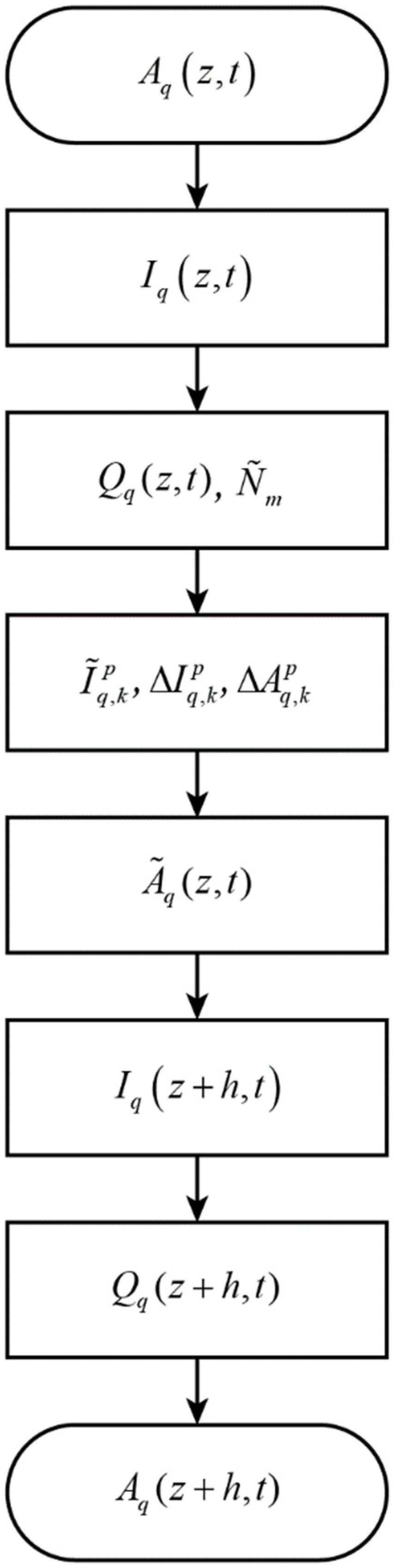
6. The New Algorithm for Calculating the Nonlinear Operator of the SSFM for Solving a System of Coupled GNLSE

When simulating the propagation of orthogonally polarized modes in polarization-maintaining optical fiber, it can be assumed that ${\gamma }_m={\gamma }_n=\gamma$. Taking this into account, we write (19) according to (3) in the following form:

$$\frac{\partial A_m}{\partial z}=-\frac{\gamma }{{\omega }_0}\left({\left|A_m\right|}^2+\frac{1}{3}{\left|A_n\right|}^2\right)\frac{\partial A_m}{\partial t}+j\gamma A_m\left[\left({\left|A_m\right|}^2+\frac{2}{3}{\left|A_n\right|}^2\right)+\left(\frac{j}{\omega }-T_R\right)\left(\frac{\partial {\left|A_m\right|}^2}{\partial t}+\frac{1}{3}\frac{\partial {\left|A_n\right|}^2}{\partial t}\right)\right].$$

Or, considering that

$${\left|A_q\left(z,t\right)\right|}^2=I_q\left(z,t\right),$$

(27)

where q = m,n, as

$$\frac{\partial A_m}{\partial z}=-\frac{\gamma }{{\omega }_0}\left(I_m+\frac{1}{3}{I}_n\right)\frac{\partial A_m}{\partial t}+j\gamma A_m\left[\left(I_m+\frac{2}{3}{I}_n\right)+\left(\frac{j}{\omega }-T_R{A}_m\right)\left(\frac{\partial I_m}{\partial t}+\frac{1}{3}\frac{\partial I_n}{\partial t}\right)\right].$$

(28)

First, consider the first part of this equation

$$\frac{\partial A_m}{\partial z}=-\frac{\gamma }{{\omega }_0}\left(I_m+\frac{1}{3}{I}_n\right)\frac{\partial A_m}{\partial t}.$$

Formally, its solution, by analogy with (11), can be represented as

$$A_m\left(z+h,t\right)=A_m\left(z,t\right)\exp \left[-t_h\frac{1}{A_m\left(z,t\right)}\frac{\partial A_m\left(z,t\right)}{\partial t}\right].$$

$$t_h=h\frac{\gamma }{{\omega }_0}\left[I_m\left(z,t\right)+\frac{1}{3}{I}_n\left(z,t\right)\right].$$

(29)

By using the SSFM, we assume the constancy of the intensities within the step along the length. Within the framework of the assumptions, this equation reduces to the advection equation, which has a solution [65]:

$$A_m\left(z+h,t\right)=A_m\left(z,t-t_h\right).$$

(30)

It is correct. According to (30), for calculations, one can use the sorting algorithm to preserve indices and approximation, for example, by cubic splines. However, it is easier and faster to find an approximate solution by the finite difference method according to the inverse difference scheme on a uniform grid:

$$A_{m,k}^{p+1}=A_{m,k}^p-\frac{h}{\Delta t}\frac{\gamma }{{\omega }_0}\left(3{\tilde{I}}_{m,k}^p+{\tilde{I}}_{n,k}^p/3\right)·\Delta A_{m,k}^p.$$

(31)

Here ${\tilde{I}}_{m,k}^p,{\tilde{I}}_{n,k}^p$ are calculated according to (25), and the differences $\Delta A_{m,k}^p$ are determined as

$$\Delta A_{q,k}^p=A_{q,k}^p-A_{q,k-1}^p; k=1,2\dots N;p=1,2\dots N;q=m,n.$$

(32)

The second part of Equation (28) can be written as

$$\frac{\partial A_m}{\partial z}=j\gamma A_m\left[\left(I_m+\frac{2}{3}{I}_n\right)+\left(\frac{j}{\omega }-T_R{A}_m\right)\left(\frac{\partial I_m}{\partial t}+\frac{1}{3}\frac{\partial I_n}{\partial t}\right)\right].$$

(33)

Equation (33) includes derivatives $\partial I_q/\partial t$. Let us express them in derivatives $\partial I_q/\partial z$ using the equations for the system’s intensity (21). From (21), we obtain a system of two equations

$$\frac{\partial I_m}{\partial z}+\frac{{\gamma }_m}{{\omega }_0}\left[\left(3I_m+\frac{1}{3}{I}_n\right)\frac{\partial I_m}{\partial t}+\frac{2}{3}{I}_m\frac{\partial I_n}{\partial t}\right]=0,$$

(34)

$$\frac{\partial I_n}{\partial z}+\frac{{\gamma }_n}{{\omega }_0}\left[\left(3I_n+\frac{1}{3}{I}_m\right)\frac{\partial I_n}{\partial t}+\frac{2}{3}{I}_n\frac{\partial I_m}{\partial t}\right]=0.$$

Solving this system for the sought derivatives, we obtain a solution in the form:

$$\frac{\partial I_m}{\partial t}=C_{m,m}\left(I_m,I_n\right)\frac{\partial I_m}{\partial z}+C_{m,n}\left(I_m,I_n\right)\frac{\partial I_n}{\partial z},$$

(35)

$$\frac{\partial I_n}{\partial t}=C_{n,m}\left(I_m,I_n\right)\frac{\partial I_m}{\partial z}+C_{n,n}\left(I_m,I_n\right)\frac{\partial I_n}{\partial z}.$$

Substituting (35) into (28), we obtain

$$\frac{1}{A_m}\frac{\partial A_m}{\partial z}=-t_h\frac{1}{A_m}\frac{\partial A_m}{\partial t}+N_m+b_{m,m}\frac{1}{I_m}\frac{\partial I_m}{\partial z}+b_{m,n}\frac{1}{I_n}\frac{\partial I_n}{\partial z}.$$

(36)

or [66]

$$\frac{\partial \left[\ln \left(A_m\right)\right]}{\partial z}-b_{m,m}\frac{\partial \left[\ln \left(I_m\right)\right]}{\partial z}+b_{m,n}\frac{\partial \left[\ln \left(I_n\right)\right]}{\partial z}=-t_h\frac{1}{A_m}\frac{\partial A_m}{\partial t}+N_m.$$

Or

$$\frac{\partial \left\{\ln \left[A_m/Q\right]\right\}}{\partial z}=-t_h\frac{1}{A_m}\frac{\partial A_m}{\partial t}+{\tilde{N}}_m.$$

(37)

Here

$${\tilde{N}}_m=j\gamma A_m\left(I_m+\frac{2}{3}{I}_n\right),$$

(38)

$$Q_m=I_m^{b_{m,m}}·I_n^{b_{m,n}},$$

(39)

$$b_{m,n}=\left(1+j{T}_R{\omega }_0\right)\frac{I_m\left(\frac{1}{3}{I}_m+2\frac{7}{9}{I}_n\right)}{8\frac{2}{3}{I}_m{I}_n+I_m^2+I_n^2}.$$

(40)

From (36), it follows that

$$\frac{A_m(z+h,t)}{Q_m(z+h,t)}=\frac{A_m(z,t)}{Q_m(z,t)}\exp \left({\tilde{N}}_m\right)\exp \left[-t_h\frac{1}{A_m\left(z,t\right)}\frac{\partial A_m\left(z,t\right)}{\partial t}\right].$$

(41)

Let

$${\tilde{A}}_m(z,t)=A_m(z,t)\exp \left[-t_h\frac{1}{A_m\left(z,t\right)}\frac{\partial A_m\left(z,t\right)}{\partial t}\right],$$

(42)

then according to (41), what can write the solution to Equation (27) in the form:

$$A_m(z+h,t)={\tilde{A}}_m(z,t)\frac{Q_m(z+h,t)}{Q_m(z,t)}\exp \left({\tilde{N}}_m\right).$$

(43)

The intensities $I_m\left(z+h,t\right),I_n\left(z+h,t\right)$ necessary to determine the function $Q_m(z+h,t)$ by Equation (37) we find by solving the system (33) using the finite differences method. For this, we use a simple finite-difference scheme of inversely directed differences on a uniform grid (22). The same scheme, taking into account (30), (32), and (40), we use to calculate ${\tilde{A}}_q(z,t)$.

Thus, we obtain the following algorithm for the execution of the nonlinear operator in SSFM.

1. According to (27), we calculate the intensities $I_q\left(z,t\right)$.

2. Using Equations (38)–(41), we calculate the functions $Q_q(z,t)$ and ${\tilde{N}}_m$.

3. Calculate the intensities at the nodes ${\tilde{I}}_{q,k}^p$ and the difference $\Delta I_{q,k}^p$$\Delta A_{q,k}^p$, according to (25) and (32).

4. According to (31) and (32), we compute ${\tilde{A}}_q(z,t)$.

5. Using Equation (22), we calculate $I_q\left(z+h,t\right)$.

6. Using Equations (39)–(41), we calculate the functions $Q_q(z+h,t)$.

7. According to (43), we calculate the complex envelope $A_q(z+h,t)$.

As a result, we implement SSFM as follows. Calculations are performed according to the well-known symmetric scheme. We execute the linear operator as usual, without any changes. All changes relate exclusively to the nonlinear operator. We present the algorithm for executing a nonlinear operator in Figure 1.

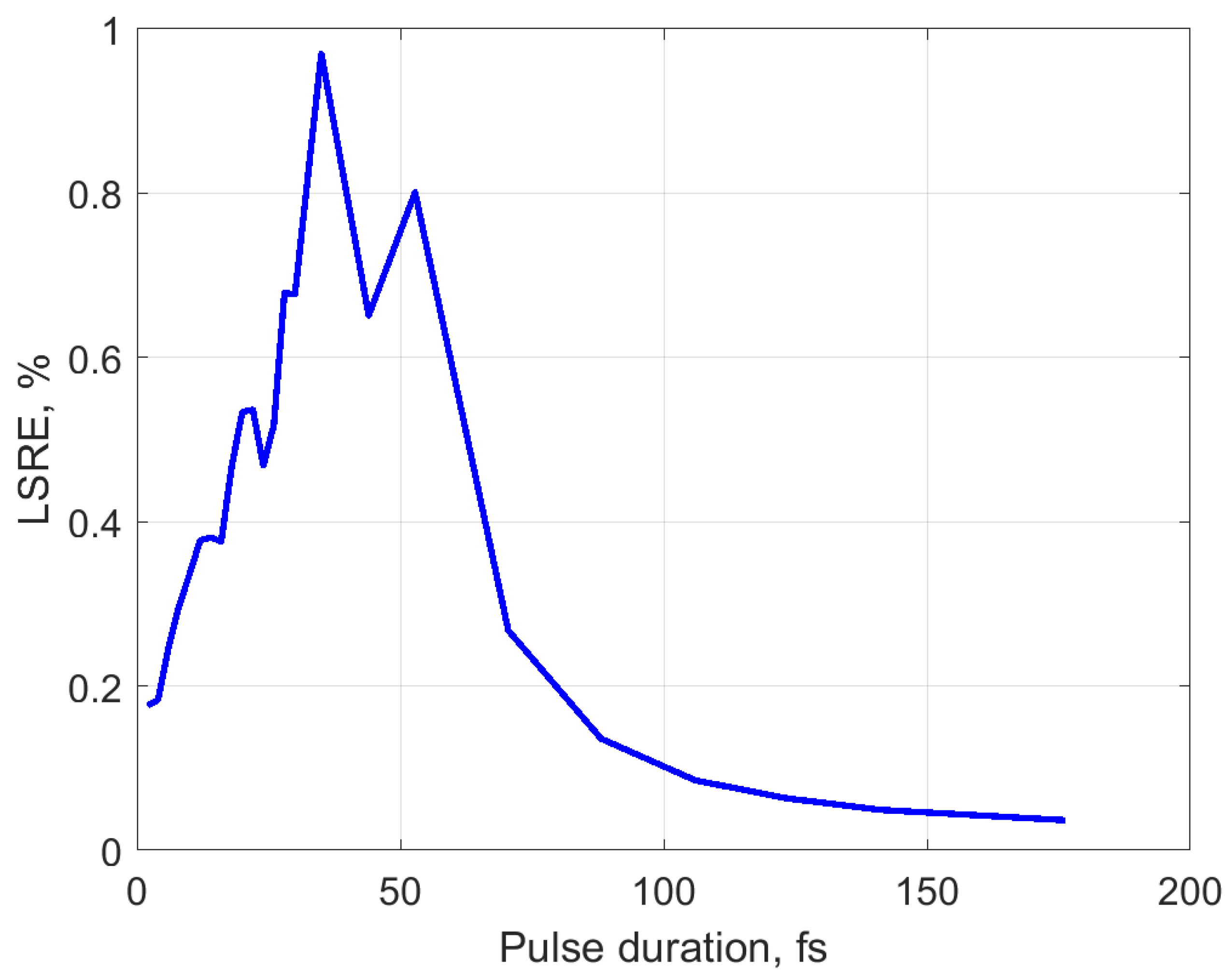
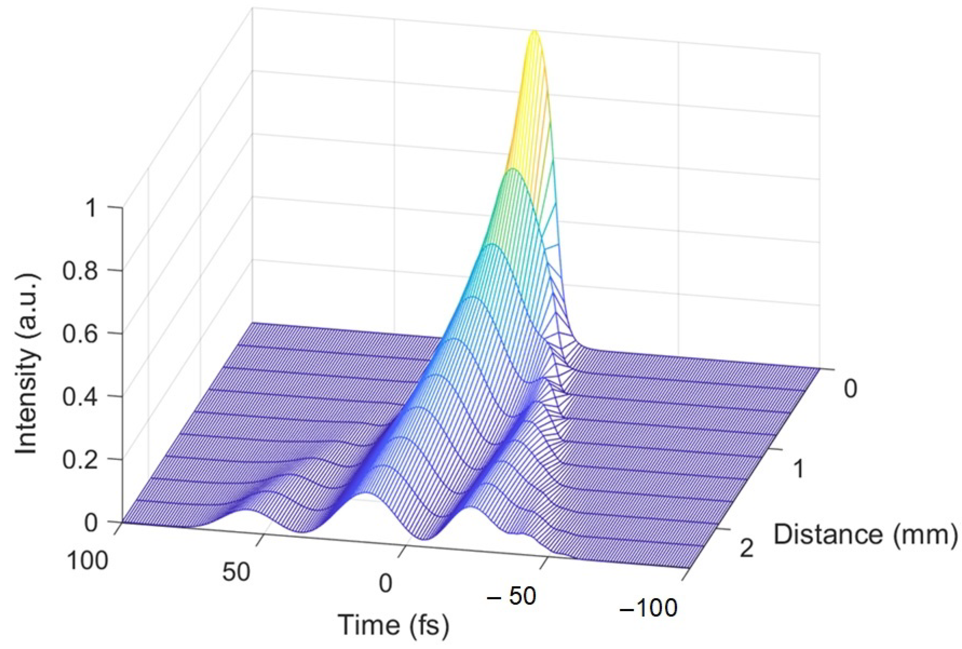
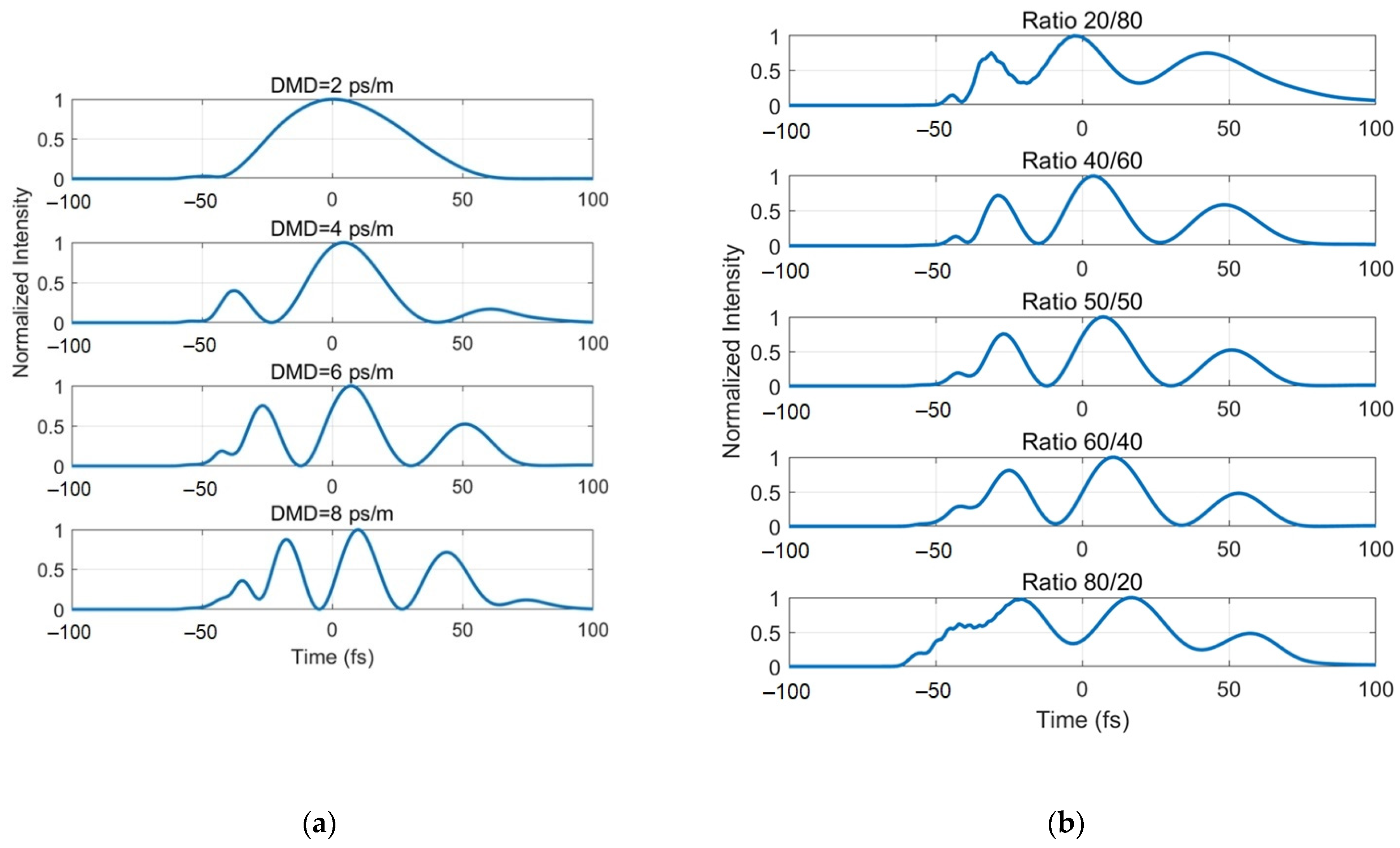
7. Results of Simulation of the Propagation of a High-Power Femtosecond Optical Pulse in a Single-Mode Polarization-Maintaining Optical Fiber

To test the proposed algorithm for the execution of the nonlinear operator GSSFM, welet us compare the simulation results obtained, with the results obtained using the well-known algorithm [55] for executing a nonlinear operator, based on the numerical solution of the system of Madelung equations directly. We simulated the response at the polarization-maintaining optical fiber output to the action at the fiber input of an ultrashort sech²-shaped pulse without a chirp. The peak power of the pulse is 100 kW and the duration 10 fs. The length of fiber is 2 mm. We assume that the excitation of polarization modes at the input is uniform. An optical fiber with the following parameters was considered. Mode attenuation coefficients α₁ = α₂ = 0.2 dB/km. Dispersion parameters of modes β₁₁ = 4.890 × 10⁻⁹ s/m; β₁₂ = 4.894 × 10⁻⁹ s/m; β₂₁ = β₂₂ = 3.616 × 10⁻²⁶ s²/m; β₃₁ = β₃₂ = 2.750 × 10⁻⁴¹ s³/m. The differential mode delay is was 4 ps. The nonlinearity and Raman scattering parameters were assumed to be γ = 2.42 W⁻¹/km and T = 3 fs.

Figure 2a,b presented as an example of simulation results at the time and spectral regions for an input pulse duration of 10 fs.

The error of modeling the response according to the proposed algorithm, relative to modeling the response according to the known algorithm, was estimated as the least square relative error (LSRE), which was calculated in the range of changes by the formula [58,59]:

$$LSRE=100·\sqrt{\frac{1}{N}{\displaystyle \sum _{i=1}^N{\left(\frac{y_i^a-y_i^d}{y_i^d}\right)}^2}},$$

(44)

where $y_i^d$—valid data; $y_i^a$—approximating data; N—number of points.

In this paper, the comparison we carry out in a time domain under condition $\left|A\left(t\right)\right|>0.1·\max \left[\left|A\left(t\right)\right|\right]$, where $A\left(t\right)$—is a simulated response by a known algorithm. Under calculation by Equation (44), we consider the simulation results by the known algorithm as valid data and the results of simulation by the proposed algorithm we use as approximating data. The simulation and calculation of the error estimations were executed for the responses of the time domains depending on input pulse duration. Figure 3 shows the LSRE dependence on input pulse duration.

With an increase in the duration of the input pulses, the errors first increase and reach their maximum values at durations of 30–50 fs. Then, with an increase in the duration of the input pulses, the errors decrease monotonically. As expected, the discrepancy between the simulation results for the proposed improved algorithm and that presented in [55] decreases with increasing pulse duration. With an increase in the pulse duration in the equations of the system, the contribution of the components that take into account Raman scattering of light decreases. For durations exceeding ten ps, they can be neglected. In this case, GNLSE boils down to the standard NLSE [13] and both of the above algorithms to the standard SSFM. With a decrease in the few-cycle pulse duration, the number of cycles decreases, and, accordingly, the influence of the phase on the evolution of the amplitude of the complex envelope decreases. The main difference between the considered algorithms is how they account for the evolution of the complex envelope phase. Consequently, for few-cycle pulses, with a decrease in the pulse duration, the difference between the results by using the considered algorithms also decreases. It should be noted here that with a decrease in the pulse duration as it approaches the period of the carrier oscillation, the error of theoretical estimates of the model based on the GNLSE increases in particular since the requirement the SVEA is violated.

As demonstrated by the simulation results, estimates of errors LSRE in the entire range of input pulse durations do not exceed 1%. At the same time and, under similar conditions, the computing time, according to the proposed algorithm, is reduced in comparison with the known one, by more than four times.

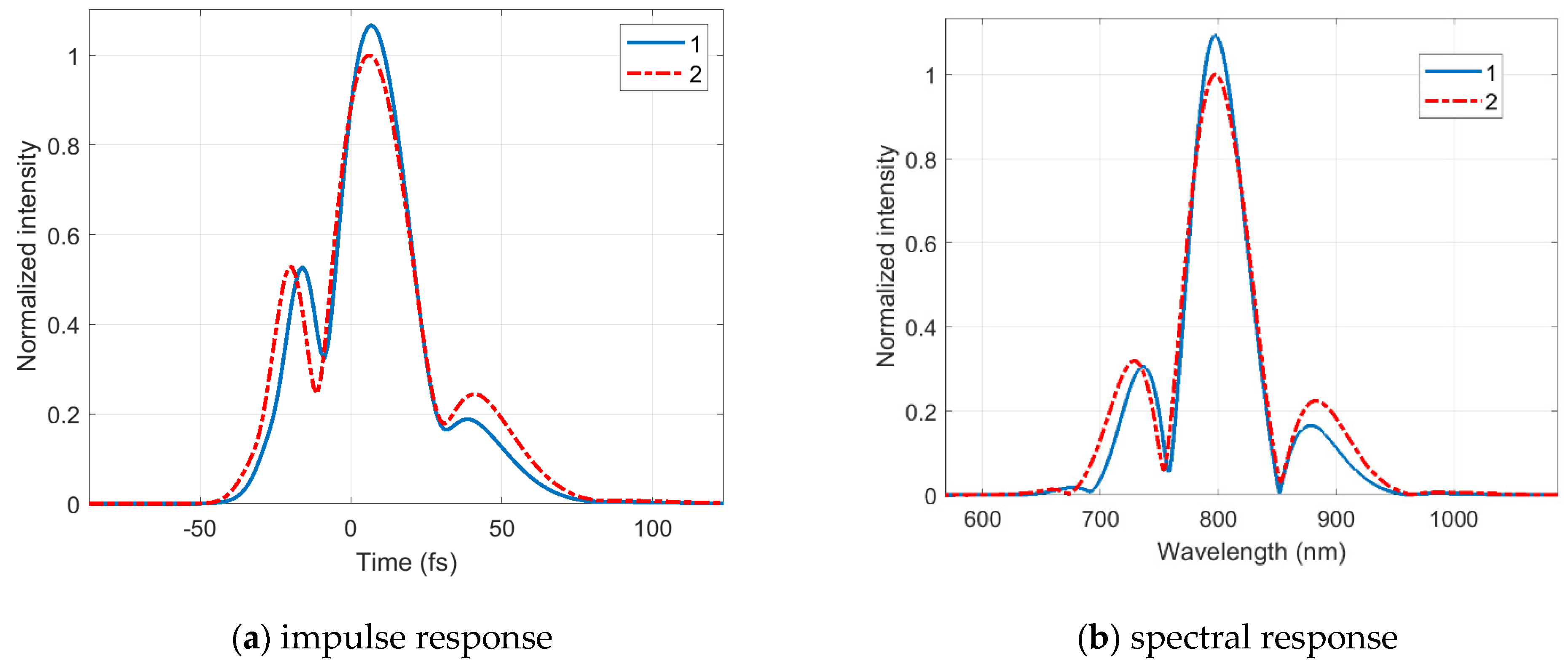
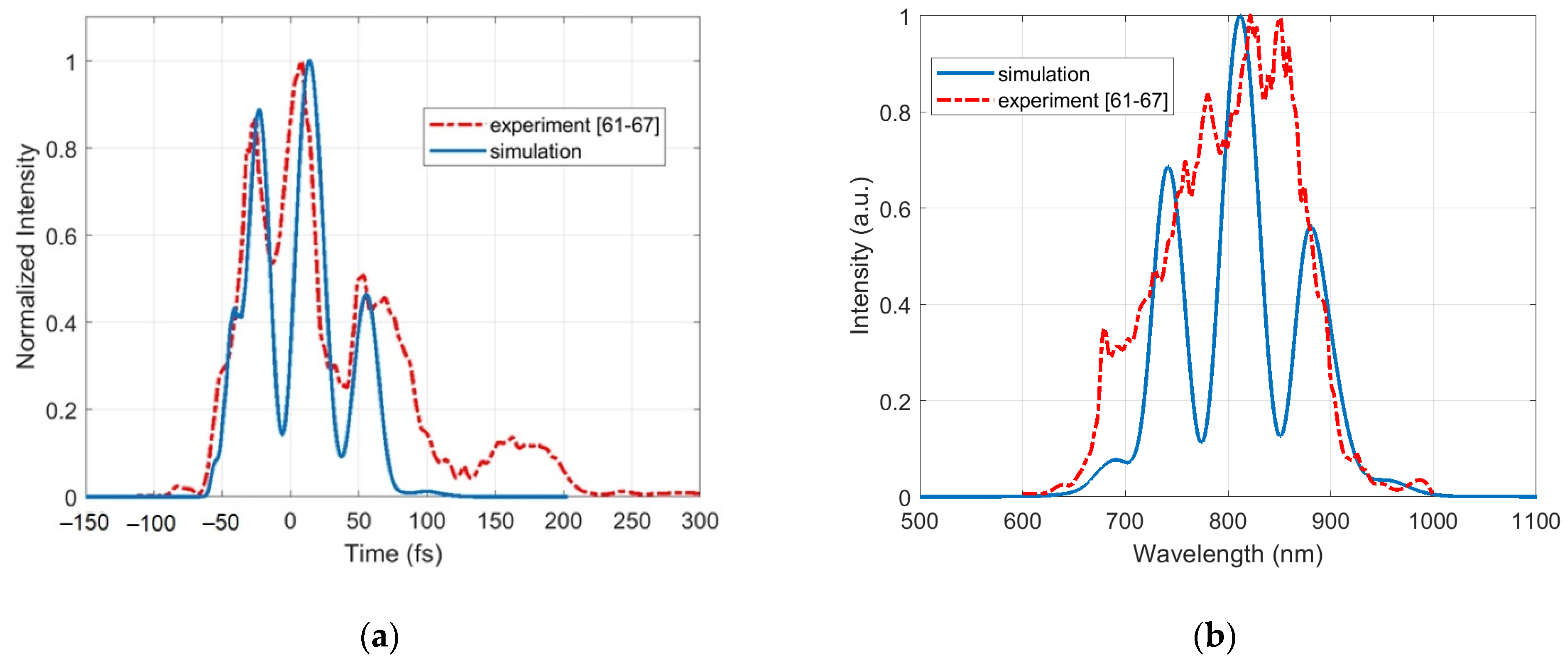
8. Compare Simulation Results with Experimental Data

To test the solution under consideration, which describes the propagation of a high-power ultrashort pulse in polarization-maintaining optical fiber, we performed the simulation for the experimental conditions described in detail [60,61,62,63,64,65,66]. According to the experiment’s description, a Ti: sapphire femtosecond laser with a mode-locking and a center wavelength of 798 nm generated pulses with a duration of 12 fs and a peak power of 175 kW. Optical radiation at the laser output is separated using an optical splitter. The one part of the optical power from the mirror to feed to the spectrometer or the fringe-resolved autocorrelator. The other part is introduced into an optical fiber using an objective with a reflector. As noted in [60,61,62,63,64,65,66], the use of such lenses excluded additional chromatic dispersion. At the output of the optical fiber, optical pulses are output using the same objective. The spectrometer evaluates the optical signal’s spectral characteristic at the input and output of the optical fiber. The impulse response was measured using the fringe-resolved autocorrelator. The experimental time and spectral characteristics of optical pulses from Refs [60,61,62,63,64,65,66] are presented below, together with the simulation results.

The experiment used an F-SPV optical fiber manufactured by “Newport,” optimized for operation at a wavelength of 633 nm. It is a Bow-Tie polarized optical fiber with a length of 2.5 mm.

Table 1. Characteristics of F-SPV optical fiber.

No	Parameter	Value
1	Index Profile	Step
2	Operating Wavelength	633–780 nm
3	Cladding Diameter	125 ± 1 μm
4	Coating Diameter	245 ± 15 μm
5	Numerical Aperture	0.14–0.18
6	Fiber Type	Bow-Tie Polarization Maintaining Singlemode
7	Mode Field Diameter, Nominal	2.8–3.7 µm @633 nm
8	Maximum Attenuation	≤15 dB/km
9	Beat length	≤2 mm
10	Cut-off Wavelength	500–600 nm

shows this type of optical fiber’s main characteristics according to the specification [67]. As in [52,53], what calculated the characteristics of the “fast” mode as for an axisymmetric step-index fiber with a refractive index profile plotted along the “fast” axis of the optical fiber. The characteristics of the “slow” mode were determined as follows. The propagation velocity parameter is determined assuming that the “slow” mode propagates with a certain delay Δβ, determined by the optical fiber’s beat length. Accordingly, ${\beta }_{1,2}={\beta }_{1,1}-\Delta \beta$. Under simulation, we use follows assumptions for determining parameters of polarization-maintaining optical fibers. We considered the research data for polarization-maintaining optical fibers of Refs [16,68,69], where, as in Refs [61,62,63,64,65,66], used the same optical fiber in the experiment. Here, as in Refs [16,68,69], assume that the chromatic dispersion parameters and the nonlinearity parameter for the orthogonally polarized modes are the same. We accept that the Kerr nonlinearity coefficient n₂ = 3.5 × 10⁻²⁰ [16,70,71,72]. The Raman scattering parameter is T_R = 3 fs [54,55,73]. As a result of calculations according to [13,74] for a single-mode step-index optical fiber with the considered parameters, we obtained that β_1.1 = 4.294 × 10⁻⁹ s/m, β_2.1 = 4.290 × 10⁻⁹ s/m, β_1.2 = β_2.2 = 3.62 × 10⁻²⁶ s²/m, β_1.3 = β_2.3 = 2.75 × 10⁻⁴¹ s³/m, and γ = 4.80 W⁻¹/km. When determining the chromatic dispersion parameters, the refractive index of doped silica glass is directly proportional to the concentration of the dopant [75]. A relatively large error characterizes the estimates of the parameters of modes obtained in this way; however, they fully satisfy the data on the fiber specification [67] and, on the whole, agree with the parameters for this type of fiber used in the processing of experimental data in [16,60,61,62,63,64,65,66].

We simulated the evolution of a high-power femtosecond pulse during propagation in a polarization-maintaining optical fiber for the above experimental conditions. We simulated the pulse propagation process by solving the system of Equation (4) according to the proposed algorithm of SSFM. For example, Figure 4 shows the simulation results for uniform excitation conditions at the input and the delay between orthogonally polarized modes equal to 6 ps/m.

As a result of the simulation, we obtain impulse responses at the optical fiber output. The beat length of the optical fiber sample used in the experiment and the conditions for the modes excitation at the input are not uniquely determined. For this reason, we first calculated impulse responses versus mode delay and input power distribution between orthogonally polarized modes. Figure 5a shows examples of the pulsed responses obtained from modeling at the output of the fiber with uniform excitation of modes at the input, depending on the mode delay. Figure 5b shows examples of the pulsed responses obtained from modeling at the fiber output with a mode delay of 6 ps/m, depending on the power distribution at the input between the “fast” and “slow” orthogonally polarized modes. As follows from the graphs in Figure 5a,b, the impulse response shape significantly depends on the mode delay and input conditions. It can change significantly when these parameters are varied in the range of admissible values.

Figure 6a,b show the time-domain impulse response at the output of the optical fiber and its spectral characteristics obtained from the simulation, respectively. We obtained these dependencies with a mode delay equal to 6 ps/m and power distribution between orthogonally polarized modes at the input between ‘fast’ and ‘slow’ modes with ratio 70/30. Furthermore, Figure 6a,b shows the experimental curves from [60,61,62,63,64,65,66].

The form of the response time characteristic obtained due to modeling, according to the proposed algorithm (Figure 6a), is practically identical to that of the experimental curve. It has the shape of a glove with three distinct peaks. The time delay between the main peaks of the experimental curve is 33.5 fs (Figure 6a). On the other hand, the time delay between the main peaks of the theoretical curve is 36.0 fs (Figure 6a). Therefore, the differences in the estimates of the time intervals between the maximum values of the glove peaks, determined by the theoretical and experimental characteristics, do not exceed 8%. The spectrum width at the level of 0.5 for the experimental characteristic is 143.8 nm (Figure 6b). On the other hand, the spectrum width at the level of 0.5 for the theoretical curve is 159.4 nm (Figure 6b). Thus, the difference in the estimates of the spectral width obtained experimentally, and modeled using the algorithm proposed in this work, is no more than 11%.

We must note that the parameters of the Kerr nonlinearity and Raman scattering of light significantly affect the action of high-power pulses. However, these parameters are not presented in the passports of the optical fibers. Therefore, as a rule, some average values for silica fibers, in general, are taken in the calculations. Also, the dispersion characteristic parameters of the polarization modes are not measured and indicated in the passports of polarization-maintaining optical fibers. These values are either calculated from the design characteristics of the fiber or are taken to be the same as for fibers of a similar type from the publications. With such an uncertainty in the initial data, the 10–15% difference between theoretical and experimental data is an excellent result.

The error of the obtained theoretical estimates relative to the experimental ones significantly exceeds the difference in the simulation results obtained by solving the GNLSE using different SSFM algorithms. First, this is due to the approximations of the model described by the GNLSE system. In particular, it assumes that the SVEA conditions are satisfied, there is no wave scattering at large angles, and the divergence of the electric field is small. In addition, this is undoubtedly due to errors of the method and algorithms used to solve the GNLSE system. However, in our opinion, the most significant contribution was made by the uncertainty of the initial data. It should be noted that the parameters of the Kerr nonlinearity and Raman scattering of light significantly affect the action of high-power pulses. However, these parameters are not specified in the optical fiber datasheets. Therefore, as a rule, some average values for silica fibers are taken in the calculations. According to [76], the nonlinear refraction coefficient of a silica optical fiber, doped by Germanium, depending on the concentration of the dopant, is n₂ = 2.47 × 10⁻²⁰–3.32 × 10⁻²⁰ m²/W. The Raman scattering parameter of silica optical fibers can be taken equal to 3 ± 1 fs [73]. Thus, the spread of possible values of these parameters reaches 30% and more. Furthermore, the dispersion characteristic parameters of the polarization modes are not measured and indicated in the passports of polarization-maintaining optical fibers. These values are either calculated from the design characteristics of the fiber or are taken to be the same as for fibers of a similar type from the publications. With such an uncertainty in the initial data (up to 30%), the 10–15% difference between theoretical and experimental data is a good result.

9. Conclusions

The article proposes an SSFM implementation algorithm for solving a coupled GNLSE system to simulate the evolution of high-power ultrashort pulse propagation in a birefringent optical fiber. The algorithm is based on a well-known solution based on the application of the Madelung transform for nonlinear operator execution. In the presented work, from the equations of the Madelung system concerning intensities, the derivatives of intensities to time were expressed in terms of derivatives to distance. This made it possible to obtain a system of equations that eliminates the need for the numerical solution of differential equations, concerning the phases of complex envelopes when performing a nonlinear operator. As a result, as shown by the simulation results, the proposed algorithm reduces the computation time during simulation compared to the known one, based on the numerical solution of Madelung’s equations when the nonlinear operator is executed, by more than four times. Comparison of the simulation results obtained using the proposed and well-known algorithms showed that estimates of errors LSRE in the considered range of input pulse durations do not exceed 1%. At the same time and, under similar conditions, the computing time, according to the proposed algorithm, is reduced in comparison with the known one, by more than four times. All of the above allows us to conclude that the developed SSFM implementation algorithm can be used to solve the coupled GNLSE system to simulate the evolution of a high-power ultrashort pulse propagating in a birefringent optical fiber.

References

1. Anscombe, N. Femtosecond Future. Nat. Photon 2010, 4, 158. [Google Scholar] [CrossRef]
2. Sibbett, W.; Lagatsky, A.A.; Brown, C.T.A. The Development and Application of Femtosecond Laser Systems. Opt. Express OE 2012, 20, 6989–7001. [Google Scholar] [CrossRef] [PubMed]
3. Sugioka, K. Progress in Ultrafast Laser Processing and Future Prospects. Nanophotonics 2017, 6, 393–413. [Google Scholar] [CrossRef] [Green Version]
4. Li, B.; Zhang, D.; Liu, J.; Tian, Y.; Gao, Q.; Li, Z. A Review of Femtosecond Laser-Induced Emission Techniques for Combustion and Flow Field Diagnostics. Appl. Sci. 2019, 9, 1906. [Google Scholar] [CrossRef] [Green Version]
5. Debord, B.; Gérôme, F.; Paul, P.-M.; Husakou, A.; Benabid, F. 2.6 MJ Energy and 81 GW Peak Power Femtosecond Laser-Pulse Delivery and Spectral Broadening in Inhibited Coupling Kagome Fiber. In Proceedings of the 2015 Conference on Lasers and Electro-Optics (CLEO), San Jose, CA, USA, 10–15 May 2015; pp. 1–2. [Google Scholar]
6. Fu, W.; Wright, L.G.; Wise, F.W. High-Power Femtosecond Pulses without a Modelocked Laser. Optica 2017, 4, 831–834. [Google Scholar] [CrossRef] [PubMed]
7. Chung, H.-Y.; Liu, W.; Cao, Q.; Song, L.; Kärtner, F.X.; Chang, G. Megawatt Peak Power Tunable Femtosecond Source Based on Self-Phase Modulation Enabled Spectral Selection. Opt. Express 2018, 26, 3684–3695. [Google Scholar] [CrossRef]
8. Larson, A.M.; Yeh, A.T. Delivery of Sub-10-Fs Pulses for Nonlinear Optical Microscopy by Polarization-Maintaining Single Mode Optical Fiber. Opt. Express 2008, 16, 14723–14730. [Google Scholar] [CrossRef]
9. Le, T.; Tempea, G.; Cheng, Z.; Hofer, M.; Stingl, A. Routes to Fiber Delivery of Ultra-Short Laser Pulses in the 25 Fs Regime. Opt. Express 2009, 17, 1240–1247. [Google Scholar] [CrossRef]
10. Michieletto, M.; Lyngsø, J.K.; Jakobsen, C.; Lægsgaard, J.; Bang, O.; Alkeskjold, T.T. Hollow-Core Fibers for High Power Pulse Delivery. Opt. Express 2016, 24, 7103–7119. [Google Scholar] [CrossRef] [Green Version]
11. Kodama, Y.; Hasegawa, A. Nonlinear Pulse Propagation in a Monomode Dielectric Guide. IEEE J. Quantum Electron. 1987, 23, 510–524. [Google Scholar] [CrossRef]
12. Boyd, R.W. Nonlinear Optics, 3rd ed.; Academic Press: Amsterdam, The Netherlands; Boston, MA, USA, 2008; ISBN 978-0-12-369470-6. [Google Scholar]
13. Agrawal, G.P. Nonlinear Fiber Optics, 5th ed.; Elsevier: Amsterdam, The Netherlands; Academic Press: Cambridge, MA, USA, 2013; ISBN 978-0-12-397023-7. [Google Scholar]
14. Marcuse, D.; Manyuk, C.R.; Wai, P.K.A. Application of the Manakov-PMD Equation to Studies of Signal Propagation in Optical Fibers with Randomly Varying Birefringence. J. Lightwave Technol. 1997, 15, 1735–1746. [Google Scholar] [CrossRef] [Green Version]
15. Kalithasan, B.; Nakkeeran, K.; Porsezian, K.; Dinda, P.T.; Mariyappa, N. Ultra-Short Pulse Propagation in Birefringent Fibers—the Projection Operator Method. J. Opt. A Pure Appl. Opt. 2008, 10, 085102. [Google Scholar] [CrossRef]
16. Mumtaz, S.; Essiambre, R.-J.; Agrawal, G.P. Nonlinear Propagation in Multimode and Multicore Fibers: Generalization of the Manakov Equations. J. Lightwave Technol. 2013, 31, 398–406. [Google Scholar] [CrossRef] [Green Version]
17. Fedoruk, M.P.; Sidelnikov, O.S. Algorithms for Numerical Simulation of Optical Communication Links Based on Multimode Fiber. Comput. Technol. 2015, 20, 105–119. [Google Scholar]
18. Wang, T. Maximum Norm Error Bound of a Linearized Difference Scheme for a Coupled Nonlinear Schrödinger Equations. J. Comput. Appl. Math. 2011, 235, 4237–4250. [Google Scholar] [CrossRef] [Green Version]
19. Wang, D.; Xiao, A.; Yang, W. A Linearly Implicit Conservative Difference Scheme for the Space Fractional Coupled Nonlinear Schrödinger Equations. J. Comput. Phys. 2014, 272, 644–655. [Google Scholar] [CrossRef]
20. Dehghan, M.; Taleei, A. A Chebyshev Pseudospectral Multidomain Method for the Soliton Solution of Coupled Nonlinear Schrödinger Equations. Comput. Phys. Commun. 2011, 182, 2519–2529. [Google Scholar] [CrossRef]
21. Dehghan, M.; Abbaszadeh, M.; Mohebbi, A. Numerical Solution of System of N–Coupled Nonlinear Schrödinger Equations via Two Variants of the Meshless Local Petrov–Galerkin (MLPG) Method. Comput. Model. Eng. Sci. 2014, 100, 399–444. [Google Scholar]
22. Sakhabutdinov, A.Z.; Anfinogentov, V.I.; Morozov, O.G.; Burdin, V.A.; Bourdine, A.V.; Gabdulkhakov, I.M.; Kuznetsov, A.A. Original Solution of Coupled Nonlinear Schrödinger Equations for Simulation of Ultrashort Optical Pulse Propagation in a Birefringent Fiber. Fibers 2020, 8, 34. [Google Scholar] [CrossRef]
23. Sakhabutdinov, A.Z.; Anfinogentov, V.I.; Morozov, O.G.; Burdin, V.A.; Bourdine, A.V.; Kuznetsov, A.A.; Ivanov, D.V.; Ivanov, V.A.; Ryabova, M.I.; Ovchinnikov, V.V. Numerical Method for Coupled Nonlinear Schrödinger Equations in Few-Mode Fiber. Fibers 2021, 9, 1. [Google Scholar] [CrossRef]
24. Chen, Y.; Zhu, H.; Song, S. Multi-Symplectic Splitting Method for the Coupled Nonlinear Schrodinger Equation. Comput. Phys. Commun. 2010, 181, 1231–1241. [Google Scholar] [CrossRef]
25. Ma, Y.; Kong, L.; Hong, J.; Cao, Y. High-Order Compact Splitting Multisymplectic Method for the Coupled Nonlinear Schrödinger Equations. Comput. Math. Appl. 2011, 61, 319–333. [Google Scholar] [CrossRef]
26. Taha, T.R.; Xu, X. Parallel Split-Step Fourier Methods for the Coupled Nonlinear Schrödinger Type Equations. J. Supercomput. 2005, 32, 5–23. [Google Scholar] [CrossRef]
27. Wang, S.; Wang, T.; Zhang, L. Numerical Computations for N-Coupled Nonlinear Schrödinger Equations by Split Step Spectral Methods. Appl. Math. Comput. 2013, 222, 438–452. [Google Scholar] [CrossRef]
28. Weideman, J.a.C.; Herbst, B.M. Split-Step Methods for the Solution of the Nonlinear Schrödinger Equation. SIAM J. Numer. Anal. 1986, 23, 485–507. [Google Scholar] [CrossRef]
29. Sinkin, O.V.; Holzlohner, R.; Zweck, J.; Menyuk, C.R. Optimization of the Split-Step Fourier Method in Modeling Optical-Fiber Communications Systems. J. Lightwave Technol. 2003, 21, 61–68. [Google Scholar] [CrossRef] [Green Version]
30. Strang, G. On the Construction and Comparison of Difference Schemes. SIAM J. Numer. Anal. 1968, 5, 506–517. [Google Scholar] [CrossRef]
31. Long, V.C.; Viet, H.N.; Trippenbach, M.; Xuan, K.D. Propagation Technique for Ultrashort Pulses II: Numerical Methods to Solve the Pulse Propagation Equation. Comput. Methods Sci. Technol. 2008, 14, 13–19. [Google Scholar] [CrossRef] [Green Version]
32. Xu, X.; Taha, T. Parallel Split-Step Fourier Methods for Nonlinear Schrödinger-Type Equations. J. Math. Model. Algorithms 2003, 2, 185–201. [Google Scholar] [CrossRef]
33. Taha, T.R.; Ablowitz, M.I. Analytical and Numerical Aspects of Certain Nonlinear Evolution Equations. II. Numerical, Nonlinear Schrödinger Equation. J. Comput. Phys. 1984, 55, 203–230. [Google Scholar] [CrossRef]
34. Zhukov, V.P.; Bulgakova, N.M.; Fedoruk, M.P. Nonlinear Maxwell’s and Schrödinger Equations for Describing the Volumetric Interaction of Femtosecond Laser Pulses with Transparent Solid Dielectrics: Effect of the Boundary Conditions. J. Opt. Technol. 2017, 84, 439–446. [Google Scholar] [CrossRef]
35. Kogelnik, H. Ultrashort Pulse Propagation in Optical Fibers. In New Directions in Guided Wave and Coherent Optics; Ostrowsky, D.B., Spitz, E., Eds.; NATO ASI Series; Springer: Dordrecht, The Netherlands, 1984; pp. 43–60. ISBN 978-94-010-9550-1. [Google Scholar]
36. Mamyshev, P.V.; Chernikov, S.V. Ultrashort-Pulse Propagation in Optical Fibers. Opt. Lett. 1990, 15, 1076–1078. [Google Scholar] [CrossRef] [PubMed]
37. Lægsgaard, J. Mode Profile Dispersion in the Generalized Nonlinear Schrödinger Equation. Opt. Express 2007, 15, 16110–16123. [Google Scholar] [CrossRef]
38. Trofimov, V.A.; Stepanenko, S.; Razgulin, A. Conservation Laws of Femtosecond Pulse Propagation Described by Generalized Nonlinear Schrödinger Equation with Cubic Nonlinearity. Math. Comput. Simul. 2021, 182, 366–396. [Google Scholar] [CrossRef]
39. Copie, F.; Randoux, S.; Suret, P. The Physics of the One-Dimensional Nonlinear Schrödinger Equation in Fiber Optics: Rogue Waves, Modulation Instability and Self-Focusing Phenomena. Rev. Phys. 2020, 5, 100037. [Google Scholar] [CrossRef]
40. Kozlov, S.A.; Sazonov, S.V. Nonlinear Propagation of Optical Pulses of a Few Oscillations Duration in Dielectric Media. J. Exp. Theor. Phys. 1997, 84, 221–228. [Google Scholar] [CrossRef]
41. Maimistov, A.I. Some Models of Propagation of Extremely Short Electromagnetic Pulses in a Nonlinear Medium. Quantum Electron. 2000, 30, 287–304. [Google Scholar] [CrossRef]
42. Schäfer, T.; Wayne, C.E. Propagation of Ultra-Short Optical Pulses in Cubic Nonlinear Media. Physica D Nonlinear Phenom. 2004, 196, 90–105. [Google Scholar] [CrossRef]
43. Bespalov, V.G.; Kozlov, S.A.; Shpolyanskiy, Y.A.; Walmsley, I.A. Simplified Field Wave Equations for the Nonlinear Propagation of Extremely Short Light Pulses. Phys. Rev. A 2002, 66, 013811. [Google Scholar] [CrossRef]
44. Leblond, H.; Mihalache, D. Few-Optical-Cycle Solitons: Modified Korteweg-de Vries Sine-Gordon Equation versus Other Non--Slowly-Varying-Envelope-Approximation Models. Phys. Rev. A 2009, 79, 063835. [Google Scholar] [CrossRef] [Green Version]
45. Amiranashvili, S.; Vladimirov, A.G.; Bandelow, U. A Model Equation for Ultrashort Optical Pulses around the Zero Dispersion Frequency. Eur. Phys. J. D 2010, 58, 219–226. [Google Scholar] [CrossRef]
46. Akamine, Y.; Doan, H.D.; Fushinobu, K. Finite-Difference Time Domain Analysis of Ultrashort Pulse Laser Light Propagation under Nonlinear Coupling. J. Therm. Sci. Technol. 2013, 8, 225–239. [Google Scholar] [CrossRef] [Green Version]
47. Paasonen, V.I.; Fedoruk, M.P. Kompaktnaya dissipativnaya skhema dlya nelinejnogo uravneniya Shredingera. Comp. Tech. 2011, 16, 68–73. [Google Scholar]
48. Zayed, E.M.E.; Alurrfi, K.A.E. The G′G,1G-Expansion Method and Its Applications to Two Nonlinear Schrödinger Equations Describing the Propagation of Femtosecond Pulses in Nonlinear Optical Fibers. Optik 2016, 127, 1581–1589. [Google Scholar] [CrossRef]
49. Zayed, E.M.; Amer, Y.A. Many Exact Solutions for a Higher-Order Nonlinear Schrödinger Equation with Non-Kerr Terms Describing the Propagation of Femtosecond Optical Pulses in Nonlinear Optical Fibers. Comput. Math. Model. 2017, 28, 118–139. [Google Scholar] [CrossRef]
50. Karpik, P.A. Investigation of differnece schemes for solving the nonlinear shrodinger equation. Vestnik SSUGT. 2019, 24, 198–219. [Google Scholar] [CrossRef]
51. Amiranashvili, S.; Čiegis, R.; Radziunas, M. Numerical Methods for a Class of Generalized Nonlinear Schrödinger Equations. Kinet. Relat. Models 2015, 8, 215–234. [Google Scholar] [CrossRef]
52. Burdin, V.A.; Bourdine, A.V. Simulation results of optical pulse nonlinear few-mode propagation over optical fiber. Appl. Photonics 2016, 3, 309–320. [Google Scholar] [CrossRef]
53. Burdin, V.A.; Bourdine, A.V. Simulation of an ultrashort optical pulse propagation in a polarization-maintaining optical fiber. Appl. Photonics 2019, 6, 93–108. [Google Scholar]
54. Deiterding, R.; Glowinski, R.; Oliver, H.; Poole, S. A Reliable Split-Step Fourier Method for the Propagation Equation of Ultra-Fast Pulses in Single-Mode Optical Fibers. J. Lightwave Technol. 2013, 31, 2008–2017. [Google Scholar] [CrossRef] [Green Version]
55. Deiterding, R.; Poole, S.W. Robust Split-Step Fourier Methods for Simulating the Propagation of Ultra-Short Pulses in Single- and Two-Mode Optical Communication Fibers. In Splitting Methods in Communication, Imaging, Science, and Engineering; Glowinski, R., Osher, S.J., Yin, W., Eds.; Scientific Computation; Springer International Publishing: Cham, Switzerland, 2016; pp. 603–625. ISBN 978-3-319-41587-1. [Google Scholar]
56. Wallstrom, T.C. On the Initial-Value Problem for the Madelung Hydrodynamic Equations. Phys. Lett. A 1994, 184, 229–233. [Google Scholar] [CrossRef]
57. Espíndola-Ramos, E.; Silva-Ortigoza, G.; Sosa-Sánchez, C.T.; Julián-Macías, I.; González-Juárez, A.; de Jesús Cabrera-Rosas, O.; Ortega-Vidals, P.; Rickenstorff-Parrao, C.; Silva-Ortigoza, R. Classical Characterization of Quantum Waves: Comparison between the Caustic and the Zeros of the Madelung-Bohm Potential. J. Opt. Soc. Am. A 2021, 38, 303–312. [Google Scholar] [CrossRef] [PubMed]
58. Chengsi, L. Least Square Method Based on Relative Error. Sci. Direct Work. 2001. Available online: https://papers.ssrn.com/sol3/papers.cfm?abstract_id=3153628 (accessed on 8 December 2021).
59. Tofallis, C. Least Squares Percentage Regression. J. Mod. Appl. Stat. Methods 2009, 7, 2–12. [Google Scholar] [CrossRef] [Green Version]
60. Karasawa, N.; Nakamura, S.; Morita, R.; Shigekawa, H.; Yamashita, M. Comparison between Theory and Experiment of Nonlinear Propagation for 4.5-Cycle Optical Pulses in a Fused-Silica Fiber. Mol. Cryst. Liq. Cryst. Sci. Technol. Sect. B Nonlinear Opt. 2000, 24, 133–135. [Google Scholar]
61. Nakamura, S.; Li, L.; Karasawa, N.; Morita, R.; Shigekawa, H.; Yamashita, M. Measurements of Third-Order Dispersion Effects for Generation of High-Repetition-Rate, Sub-Three-Cycle Transform-Limited Pulses from a Glass Fiber. Jpn. J. Appl. Phys. 2002, 41, 1369–1373. [Google Scholar] [CrossRef] [Green Version]
62. Nakamura, S.; Koyamada, Y.; Yoshida, N.; Karasawa, N.; Sone, H.; Ohtani, M.; Mizuta, Y.; Morita, R.; Shigekawa, H.; Yamashita, M. Finite-Difference Time-Domain Calculation with All Parameters of Sellmeier’s Fitting Equation for 12-Fs Laser Pulse Propagation in a Silica Fiber. IEEE Photonics Technol. Lett. 2002, 14, 480–482. [Google Scholar] [CrossRef] [Green Version]
63. Nakamura, S.; Saeki, T.; Koyamada, Y. Observation of Slowly Varying Envelope Approximation Breakdown by Comparison between the Extended Finite-Difference Time-Domain Method and the Beam Propagation Method for Ultrashort-Laser-Pulse Propagation in a Silica Fiber. Jpn. J. Appl. Phys. 2004, 43, 7015–7025. [Google Scholar] [CrossRef]
64. Nakamura, S.; Takasawa, N.; Koyamada, Y. Comparison Between Finite-Difference Time-Domain Calculation With All Parameters of Sellmeier’s Fitting Equation and Experimental Results for Slightly Chirped 12-Fs Laser Pulse Propagation in a Silica Fiber. J. Lightwave Technol. 2005, 23, 855–863. [Google Scholar] [CrossRef]
65. Nakamura, S.; Takasawa, N.; Koyamada, Y.; Sone, H.; Xu, L.; Morita, R.; Yamashita, M. Extended Finite Difference Time Domain Analysis of Induced Phase Modulation and Four-Wave Mixing between Two-Color Femtosecond Laser Pulses in a Silica Fiber with Different Initial Delays. Jpn. J. Appl. Phys. 2005, 44, 7453–7459. [Google Scholar] [CrossRef]
66. Nakamura, S. Comparison between Finite-Difference Time-Domain Method and Experimental Results for Femtosecond Laser Pulse Propagation; IntechOpen: London, UK, 2010; ISBN 978-953-307-242-5. [Google Scholar]
67. F-SPV Polarization Maintaining Fiber. Available online: https://www.newport.com/p/F-SPV (accessed on 25 April 2021).
68. Liu, Q.D.; Shi, L.; Ho, P.P.; Alfano, R.R.; Essiambre, R.-J.; Agrawal, G.P. Degenerate-Cross-Phase Modulation of Femtosecond Laser Pulses in a Birefringent Single-Mode Optical Fiber. IEEE Photonics Technol. Lett. 1997, 9, 1107–1109. [Google Scholar] [CrossRef]
69. Okamoto, K.; Hosaka, T. Polarization-Dependent Chromatic Dispersion in Birefringent Optical Fibers. Opt. Lett. 1987, 12, 290–292. [Google Scholar] [CrossRef] [PubMed]
70. Betts, R.A.; Tjugiarto, T.; Xue, Y.L.; Chu, P.L. Nonlinear Refractive Index in Erbium Doped Optical Fiber: Theory and Experiment. IEEE J. Quantum Electron. 1991, 27, 908–913. [Google Scholar] [CrossRef]
71. Milam, D. Review and Assessment of Measured Values of the Nonlinear Refractive-Index Coefficient of Fused Silica. Appl. Opt. 1998, 37, 546–550. [Google Scholar] [CrossRef]
72. Kuis, R.; Johnson, A.; Trivedi, S. Measurement of the Effective Nonlinear and Dispersion Coefficients in Optical Fibers by the Induced Grating Autocorrelation Technique. Opt. Express 2011, 19, 1755–1766. [Google Scholar] [CrossRef] [PubMed]
73. Atieh, A.K.; Myslinski, P.; Chrostowski, J.; Galko, P. Measuring the Raman Time Constant (T/Sub R/) for Soliton Pulses in Standard Single-Mode Fiber. J. Lightwave Technol. 1999, 17, 216–221. [Google Scholar] [CrossRef]
74. Snyder, A.W.; Love, J.D. Optical Waveguide Theory; Science paperbacks; Chapman and Hall: London, UK; New York, NY, USA, 1983; ISBN 978-0-412-09950-2. [Google Scholar]
75. Burdin, V.A. Algorithm for Estimation of Material Dispersion of Fused Silica Glass Optical Fibers. Proc. SPIE 2015, 9533, 95330J. [Google Scholar]
76. Wada, A.; Okude, S.; Sakai, T.; Yamauchi, R. Geo2 concentration dependence of nonlinear refractive index coefficients of silica-based optical fibers. Electron. Commun. Jpn. (Part I Commun.) 1996, 79, 12–19. [Google Scholar] [CrossRef]
Figure 1. The block diagram of nonlinear operator evaluation.
Fibers 10 00022 g001
Figure 2. The simulation results: 1—proposed algorithm; 2—known algorithm. (a) impulse response; (b) spectral response.
Fibers 10 00022 g002
Figure 3. The dependencies LSRE on the input pulse duration.
Fibers 10 00022 g003
Figure 4. Evolution of an optical pulse in an optical fiber with birefringence with uniform excitation of modes at the input and a mode delay of 6 ps/m.
Fibers 10 00022 g004
Figure 5. The simulation results of the responses at the fiber output: (a) with uniform excitation of modes per input, depending on the mode delay; (b) with a mode delay of 6 ps/m depending on the power distribution between modes at the input.
Fibers 10 00022 g005
Figure 6. The simulation results: (a) impulse response; (b) spectral characteristic.
Fibers 10 00022 g006