

Numerical Study of Mid-IR Ultrashort Pulse Reconstruction Based on Processing of Spectra Converted in Chalcogenide Fibers with High Kerr Nonlinearity


Abstract
:1. Introduction
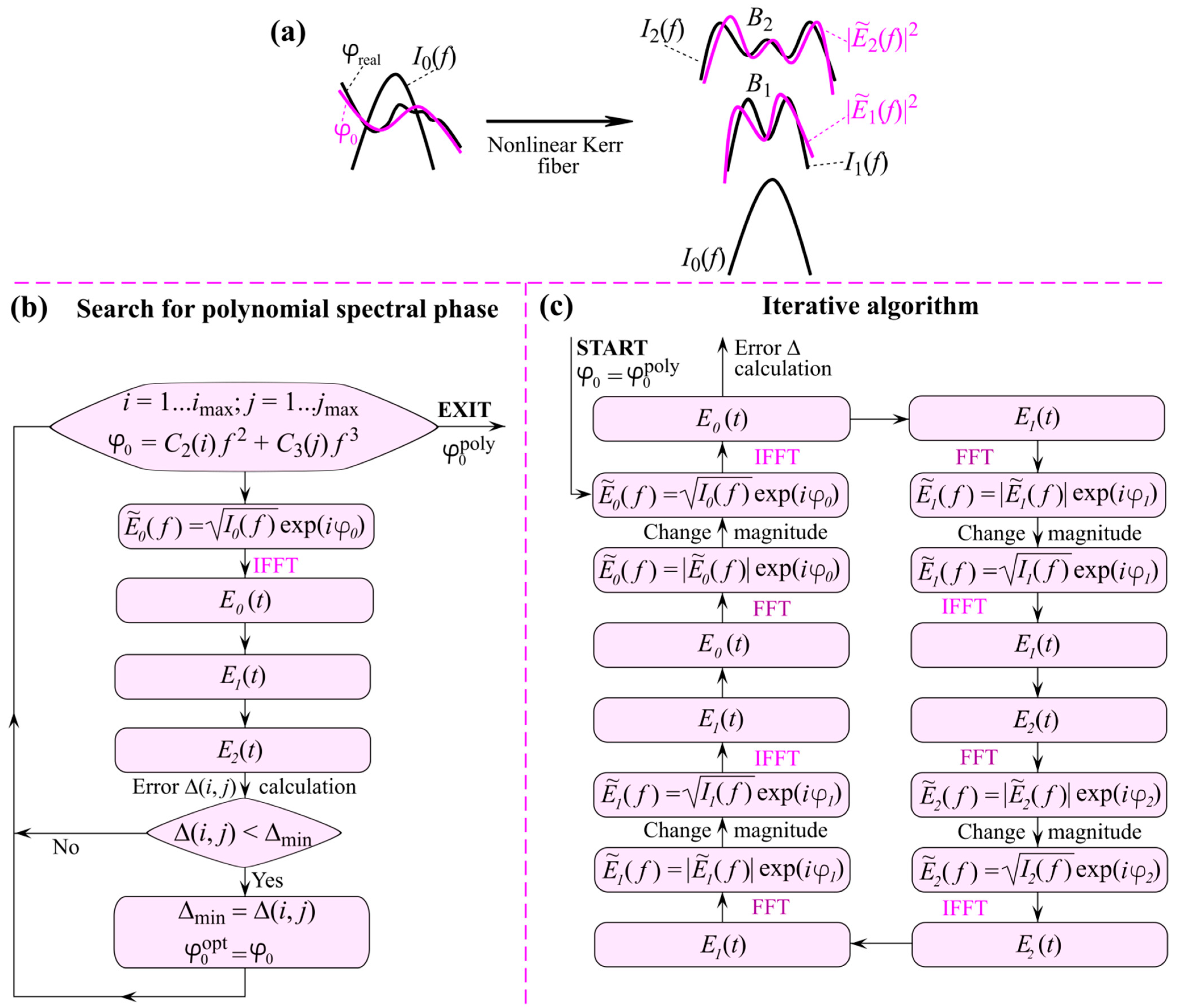
2. Methods
3. Results
3.1. Reconstruction of “Ideal” Signal
3.2. Reconstruction of Signals with Spectral Noise
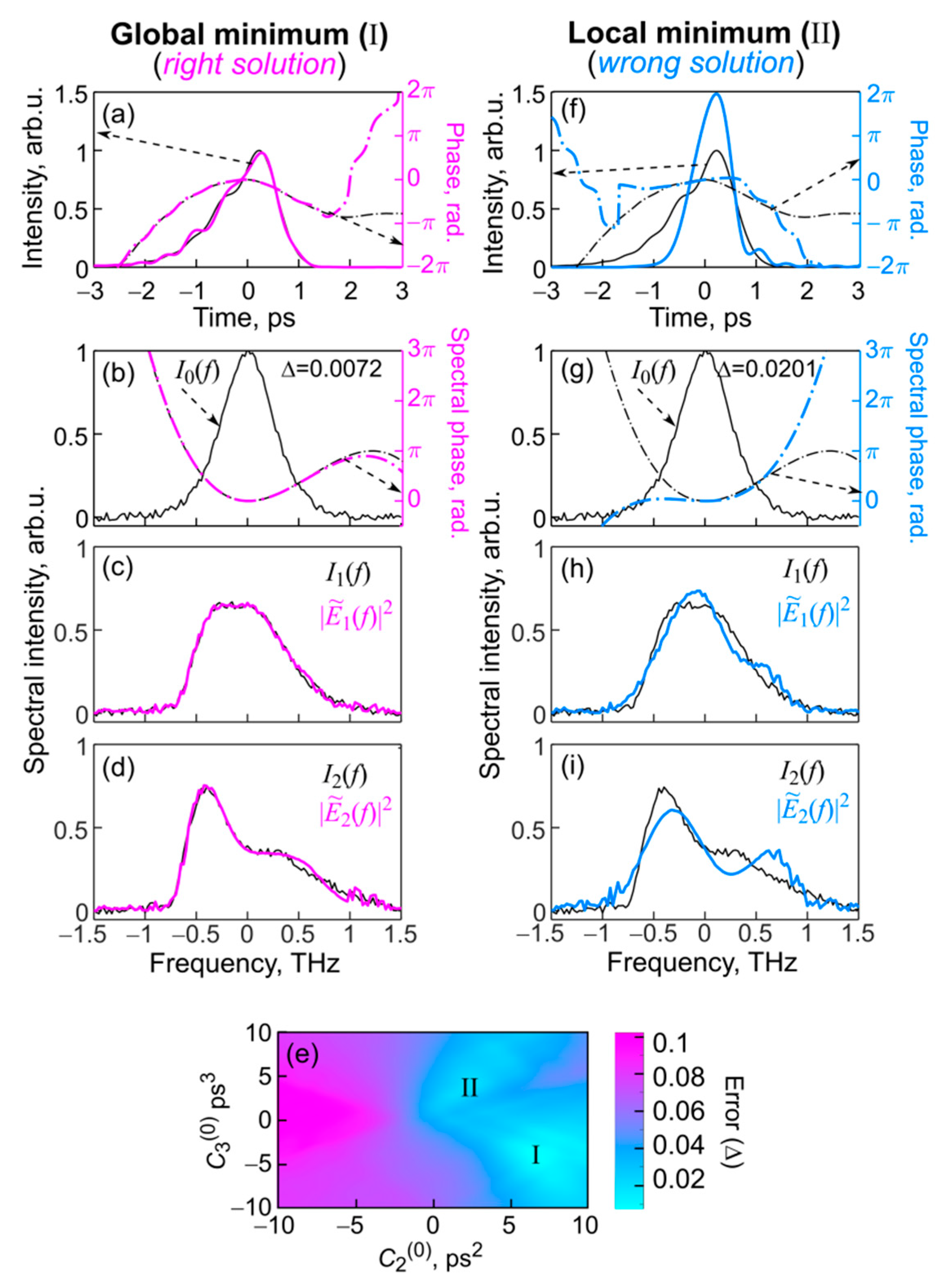
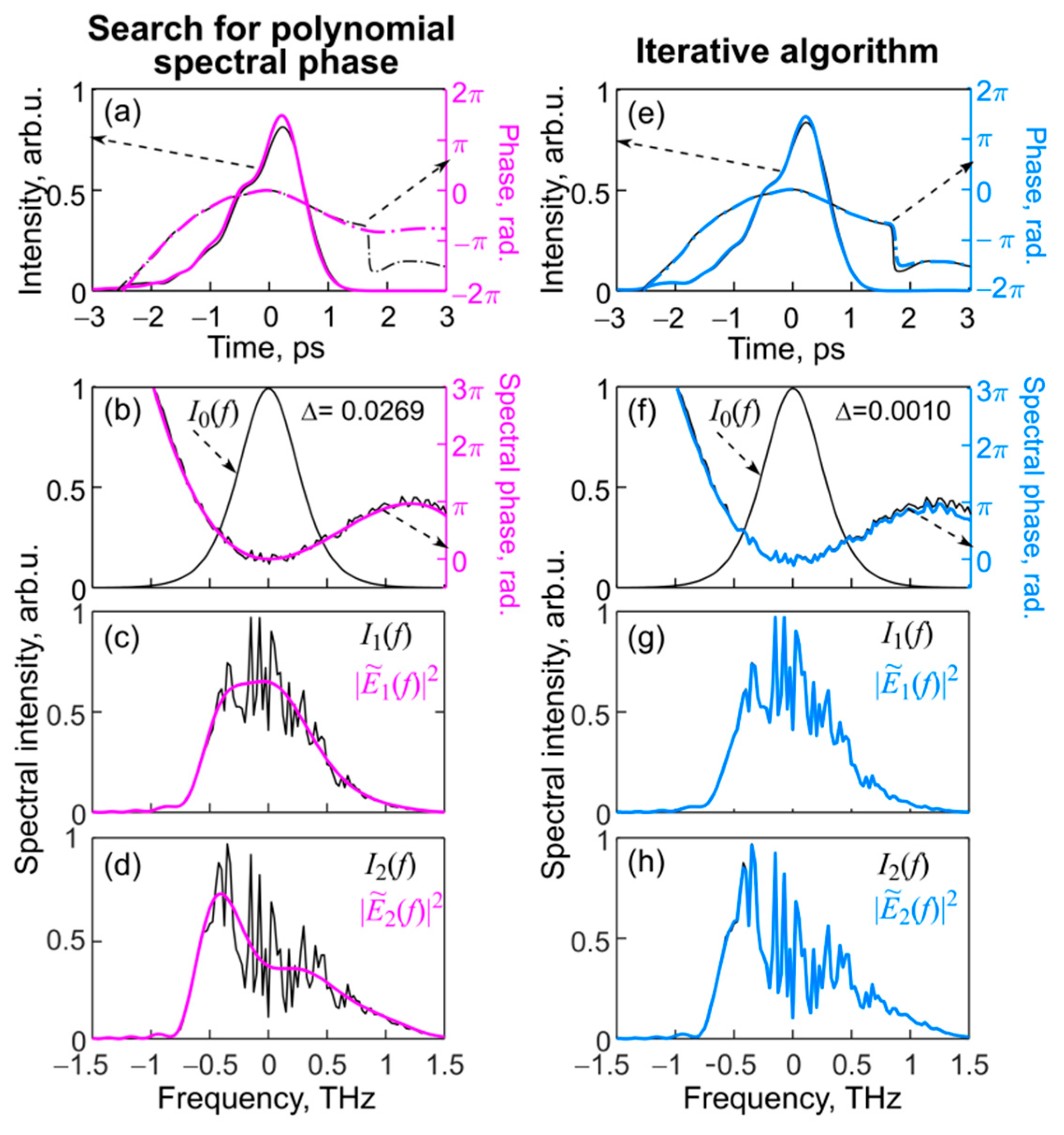
3.3. Reconstruction of Signal with Spectral Phase Perturbations
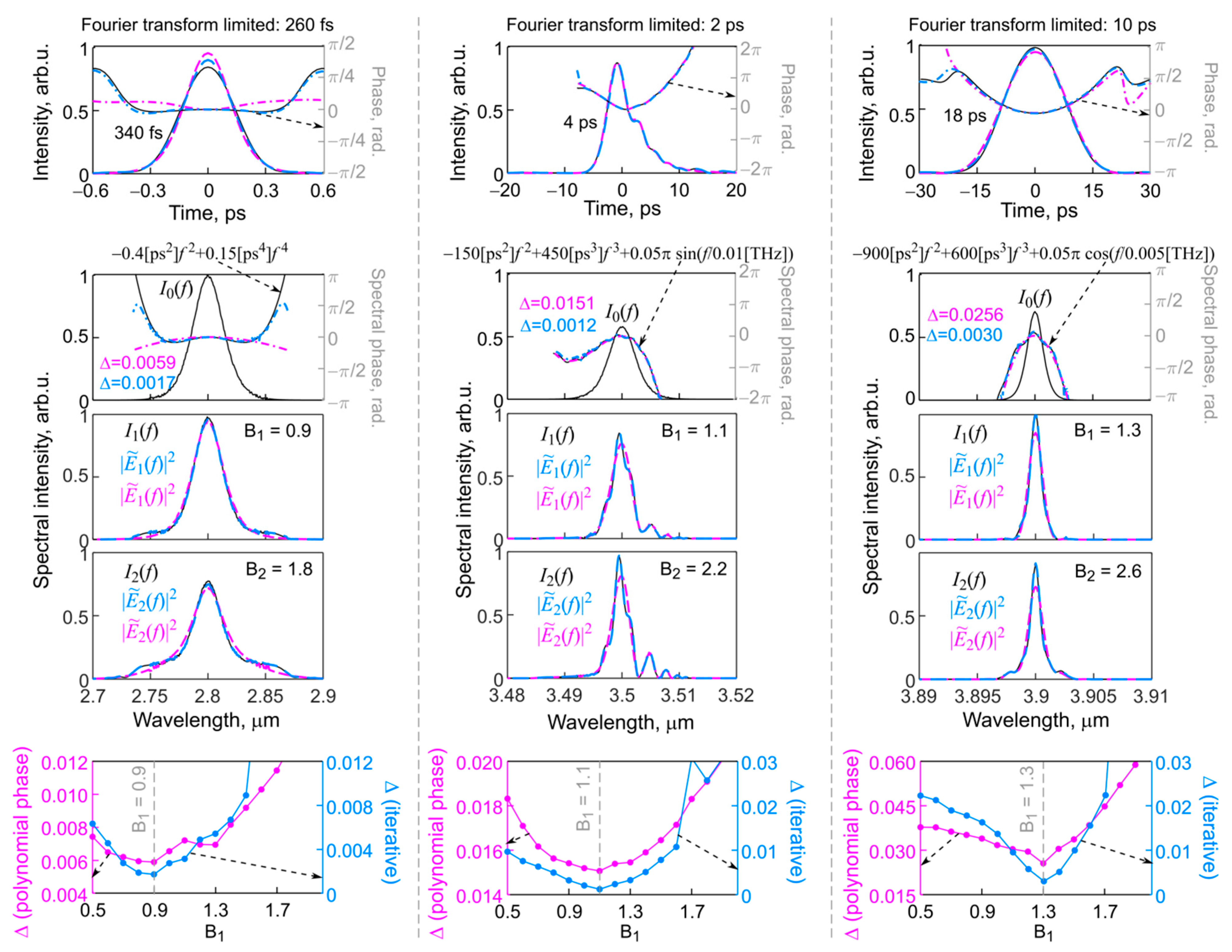
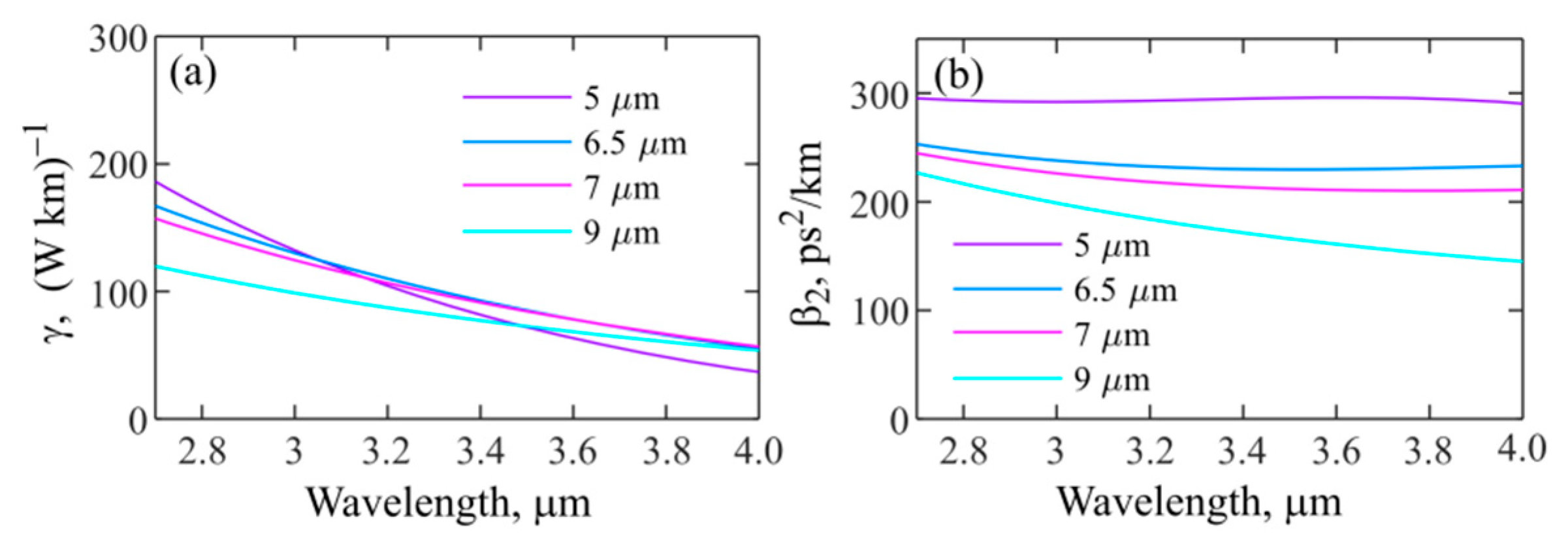
3.4. Reconstruction of Mid-IR Signals Using Chalcogenide Fiber
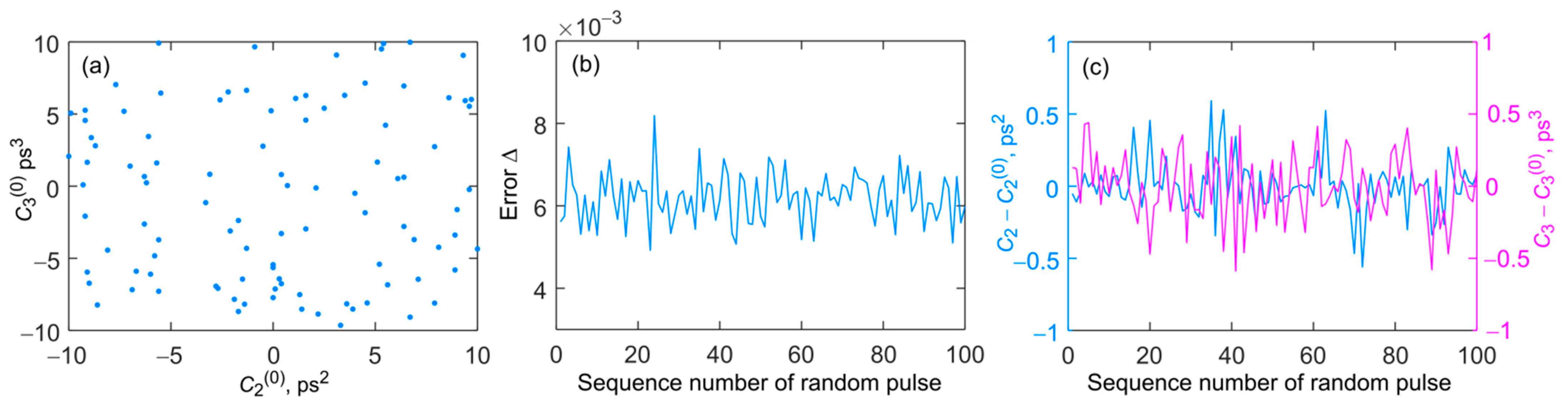
4. Discussion
5. Conclusions
Author Contributions
Funding
Institutional Review Board Statement
Informed Consent Statement
Data Availability Statement
Conflicts of Interest
References
- Trebino, R.; Jafari, R.; Akturk, S.A.; Bowlan, P.; Guang, Z.; Zhu, P.; Escoto, E.; Steinmeyer, G. Highly Reliable Measurement of Ultrashort Laser Pulses. J. Appl. Phys. 2020, 128, 171103. [Google Scholar] [CrossRef]
- Walmsley, I.A.; Dorrer, C. Characterization of Ultrashort Electromagnetic Pulses. Adv. Opt. Photonics 2009, 1, 308–437. [Google Scholar] [CrossRef]
- Trebino, R. Frequency-Resolved Optical Gating: The Measurement of Ultrashort Laser Pulses; Kluwer Academic Publishers: Boston, MA, USA, 2002. [Google Scholar]
- Zahavy, T.; Dikopoltsev, A.; Moss, D.; Haham, G.I.; Cohen, O.; Mannor, S.; Segev, M. Deep Learning Reconstruction of Ultrashort Pulses. Optica 2018, 5, 666–673. [Google Scholar] [CrossRef]
- Churkin, D.V.; Sugavanam, S.; Tarasov, N.; Khorev, S.; Smirnov, S.V.; Kobtsev, S.M.; Turitsyn, S.K. Stochasticity, Periodicity and Localized Light Structures in Partially Mode-Locked Fibre Lasers. Nat. Commun. 2015, 6, 7004. [Google Scholar] [CrossRef] [PubMed]
- Miranda, M.; Arnold, C.L.; Fordell, T.; Silva, F.; Alonso, B.; Weigand, R.; L’Huillier, A.; Crespo, H. Characterization of Broadband Few-Cycle Laser Pulses with the d-Scan Technique. Opt. Express 2012, 20, 18732–18743. [Google Scholar] [CrossRef] [PubMed]
- Pipahl, A.; Anashkina, E.A.; Toncian, M.; Toncian, T.; Skobelev, S.A.; Bashinov, A.V.; Gonoskov, A.A.; Willi, O.; Kim, A.V. High-Intensity Few-Cycle Laser-Pulse Generation by the Plasma-Wakefield Self-Compression Effect. Phys. Rev. E 2013, 87, 033104. [Google Scholar] [CrossRef]
- Geib, N.C.; Zilk, M.; Pertsch, T.; Eilenberger, F. Common Pulse Retrieval Algorithm: A Fast and Universal Method to Retrieve Ultrashort Pulses. Optica 2019, 6, 495–505. [Google Scholar] [CrossRef]
- Andrianov, A.V.; Anashkina, E.A. Asymmetric Interferometric Frequency Resolved Optical Gating for Complete Unambiguous Ultrashort Pulse Characterisation. Results Phys. 2021, 29, 104740. [Google Scholar] [CrossRef]
- Lapre, C.; Billet, C.; Meng, F.; Ryczkowski, P.; Sylvestre, T.; Finot, C.; Genty, G.; Dudley, J.M. Real-Time Characterization of Spectral Instabilities in a Mode-Locked Fibre Laser Exhibiting Soliton-Similariton Dynamics. Sci. Rep. 2019, 9, 13950. [Google Scholar] [CrossRef] [PubMed]
- Goda, K.; Jalali, B. Dispersive Fourier Transformation for Fast Continuous Single-Shot Measurements. Nat. Photon 2013, 7, 102–112. [Google Scholar] [CrossRef]
- Sugavanam, S.; Fabbri, S.; Le, S.T.; Lobach, I.; Kablukov, S.; Khorev, S.; Churkin, D. Real-Time High-Resolution Heterodyne-Based Measurements of Spectral Dynamics in Fibre Lasers. Sci. Rep. 2016, 6, 23152. [Google Scholar] [CrossRef] [PubMed]
- Anashkina, E.A.; Ginzburg, V.N.; Kochetkov, A.A.; Yakovlev, I.V.; Kim, A.V.; Khazanov, E.A. Single-Shot Laser Pulse Reconstruction Based on Self-Phase Modulated Spectra Measurements. Sci. Rep. 2016, 6, 33749. [Google Scholar] [CrossRef] [PubMed]
- Anashkina, E.A.; Andrianov, A.V.; Koptev, M.Y.; Kim, A.V. Complete Field Characterization of Ultrashort Pulses in Fiber Photonics. IEEE J. Select. Top. Quantum Electron. 2018, 24, 8700107. [Google Scholar] [CrossRef]
- Agrawal, G.P. Nonlinear Fiber Optics, 6th ed.; Elsevier: Amsterdam, The Netherlands, 2019. [Google Scholar]
- Zhu, X.; Zhu, G.; Wei, C.; Kotov, L.V.; Wang, J.; Tong, M.; Norwood, R.A.; Peyghambarian, N. Pulsed Fluoride Fiber Lasers at 3 µm [Invited]. J. Opt. Soc. Am. B 2017, 34, A15–A28. [Google Scholar] [CrossRef]
- Available online: https://irflex.com/products/irf-s-series/ (accessed on 12 September 2022).
- Available online: http://www.amorphousmaterials.com (accessed on 12 September 2022).
- Eggleton, B.J.; Luther-Davies, B.; Richardson, K. Chalcogenide Photonics. Nat. Photon. 2011, 5, 141–148. [Google Scholar] [CrossRef]
- Cai, D.; Xie, Y.; Guo, X.; Wang, P.; Tong, L. Chalcogenide Glass Microfibers for Mid-Infrared Optics. Photonics 2021, 8, 497. [Google Scholar] [CrossRef]
- Anashkina, E.A.; Andrianov, A.V.; Corney, J.F.; Leuchs, G. Chalcogenide Fibers for Kerr Squeezing. Opt. Lett. 2020, 45, 5299. [Google Scholar] [CrossRef]
- Wang, W.; Wang, K.; Li, Z.; Mao, G.; Zhang, C.; Chen, F. Linear and Third-Order Nonlinear Optical Properties of Chalcogenide Glasses within a GeS2-Sb2S3-CsCl Pseudo-Ternary System. Opt. Mater. Express 2022, 12, 1807–1816. [Google Scholar] [CrossRef]
- Anashkina, E.A.; Shiryaev, V.S.; Koptev, M.Y.; Stepanov, B.S.; Muravyev, S.V. Development of As-Se Tapered Suspended-Core Fibers for Ultra-Broadband Mid-IR Wavelength Conversion. J. Non-Cryst. Solids 2018, 480, 43–50. [Google Scholar] [CrossRef] [Green Version]


Publisher’s Note: MDPI stays neutral with regard to jurisdictional claims in published maps and institutional affiliations. |
© 2022 by the authors. Licensee MDPI, Basel, Switzerland. This article is an open access article distributed under the terms and conditions of the Creative Commons Attribution (CC BY) license (https://creativecommons.org/licenses/by/4.0/).
Share and Cite
Sorokin, A.A.; Andrianov, A.V.; Anashkina, E.A. Numerical Study of Mid-IR Ultrashort Pulse Reconstruction Based on Processing of Spectra Converted in Chalcogenide Fibers with High Kerr Nonlinearity. Fibers 2022, 10, 81. https://doi.org/10.3390/fib10100081
Sorokin AA, Andrianov AV, Anashkina EA. Numerical Study of Mid-IR Ultrashort Pulse Reconstruction Based on Processing of Spectra Converted in Chalcogenide Fibers with High Kerr Nonlinearity. Fibers. 2022; 10(10):81. https://doi.org/10.3390/fib10100081
Chicago/Turabian StyleSorokin, Arseny A., Alexey V. Andrianov, and Elena A. Anashkina. 2022. "Numerical Study of Mid-IR Ultrashort Pulse Reconstruction Based on Processing of Spectra Converted in Chalcogenide Fibers with High Kerr Nonlinearity" Fibers 10, no. 10: 81. https://doi.org/10.3390/fib10100081
APA StyleSorokin, A. A., Andrianov, A. V., & Anashkina, E. A. (2022). Numerical Study of Mid-IR Ultrashort Pulse Reconstruction Based on Processing of Spectra Converted in Chalcogenide Fibers with High Kerr Nonlinearity. Fibers, 10(10), 81. https://doi.org/10.3390/fib10100081