Thermal Boundaries in Cone Calorimetry Testing


Abstract
:1. Introduction
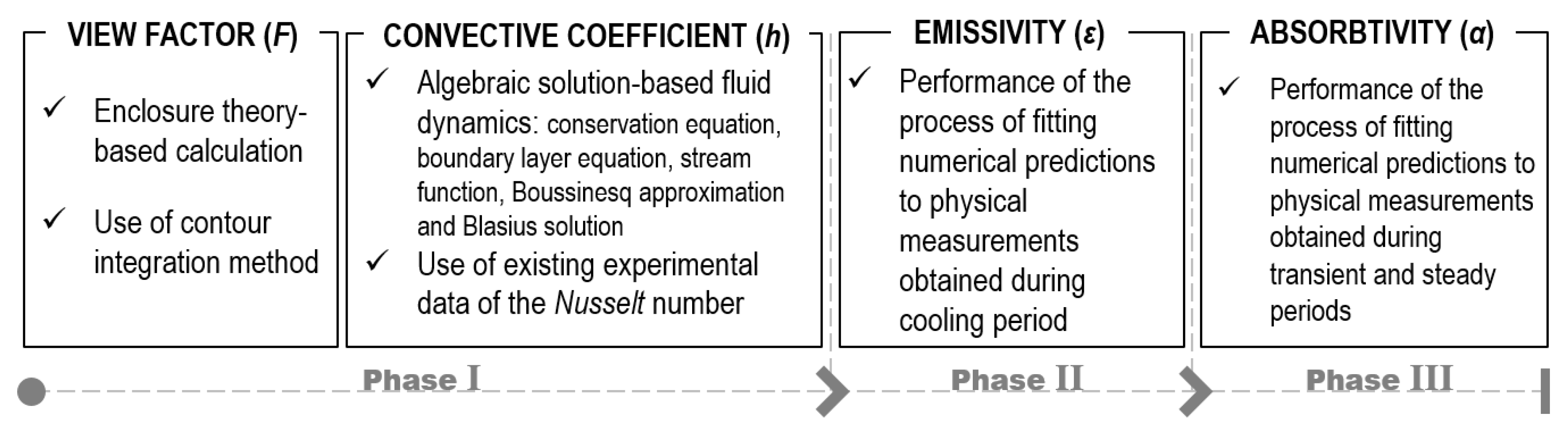
- Non-uniform distribution of irradiance on both the exposed top and side surfaces due to the truncated cone-shaped heat source. The actual quantity of this distribution is theoretically predicted by calculating geometric view factors based on the contour integration method [10];
- Radiant absorption into the surfaces. The fraction of the irradiance that is actually absorbed by the areas is represented by absorptivity. This property is strongly dependent on optical aspects, such as the nature of absorbing surfaces and spectral/directional characteristics of incident radiation. In this study, a coupled numerical–experimental process was used for its determination;
- Heat losses from the surfaces by radiant emission. This radiation transfer is represented by emissivity. This radiative property is highly case-dependent on the nature of the materials and their surface conditions. In this study, radiant heat losses were determined using a cooling test procedure;
- Heat losses from the surfaces in convection mode, which are represented by the convective coefficient. Two sets of coefficients were individually defined for the dissimilar orientations of the top and side surfaces. Their derivations are demonstrated from correlations for buoyancy-induced air flows over horizontally and vertically-oriented planes, since such thermal energy transfers are correlated with physical fluid motions driven on the solids’ boundaries.
2. Heat Transfers in Cone Calorimeter Testing
2.1. External Heat Transfers
2.1.1. Power of Heat Source
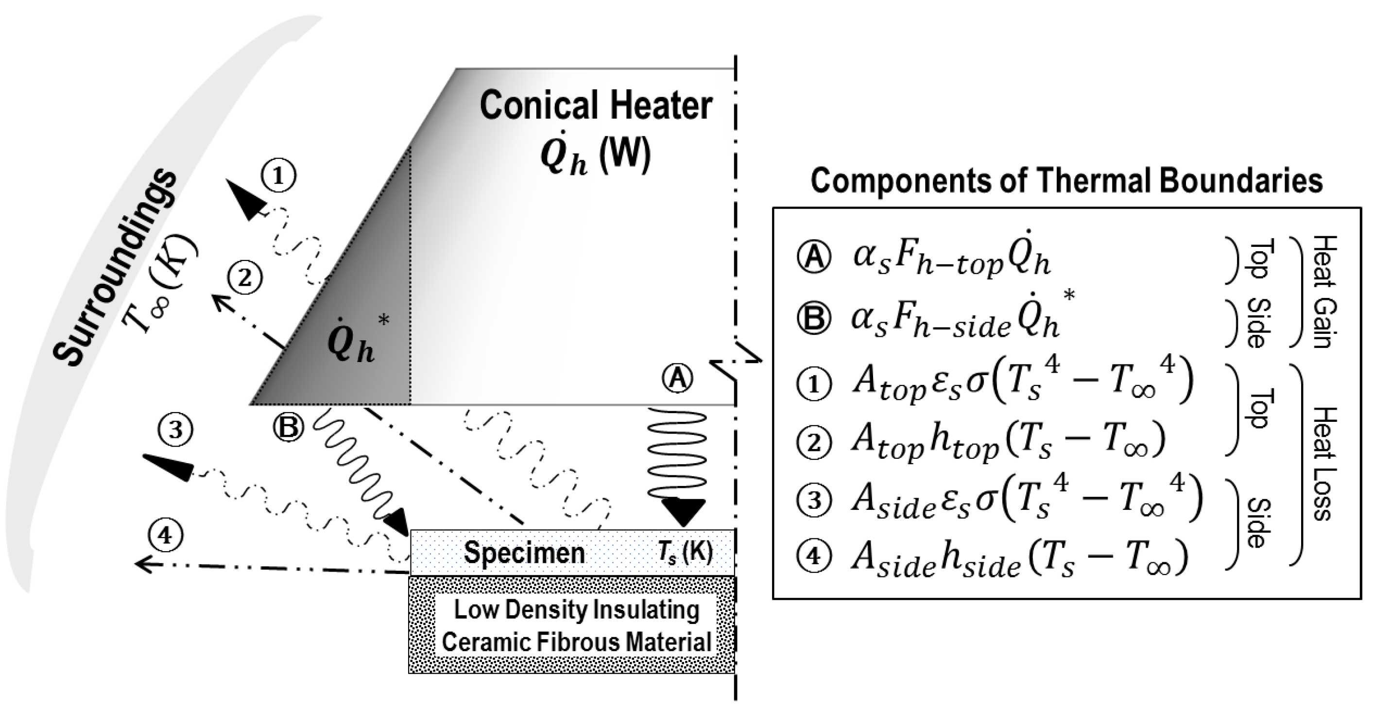
2.1.2. Radiation Absorption Mechanism (Ⓐ and Ⓑ)
2.1.3. Radiation Emission Mechanism (① and ③)
2.1.4. Convection Loss Mechanism
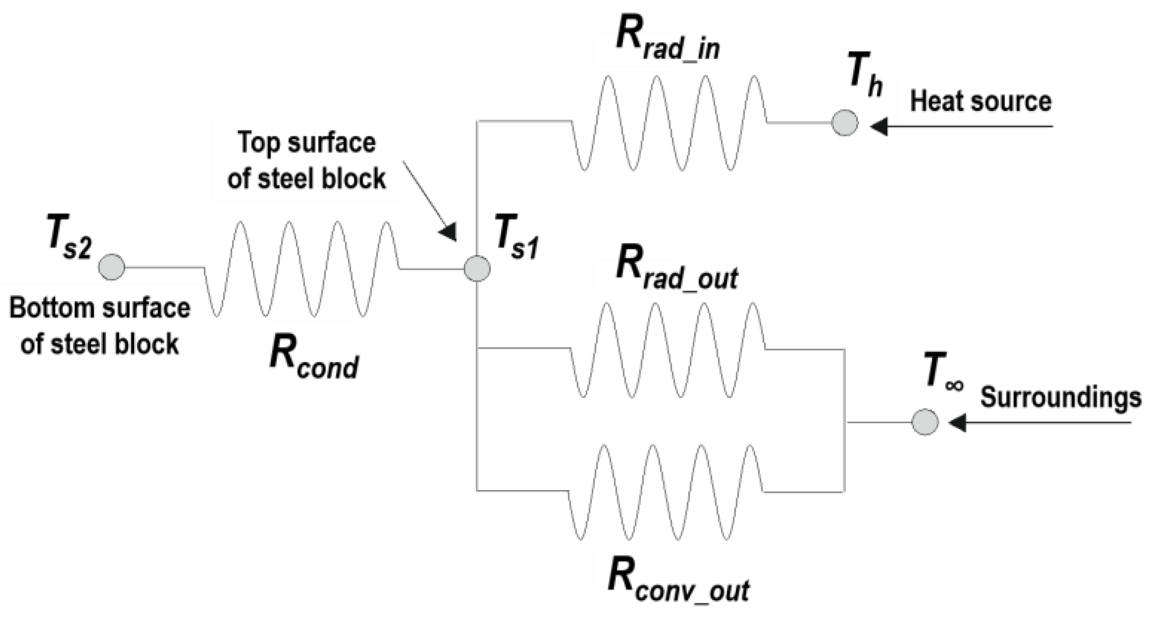
2.2. Internal Heat Transfer
2.3. Energy Balance
2.4. Determination Procedure of Key Parameters
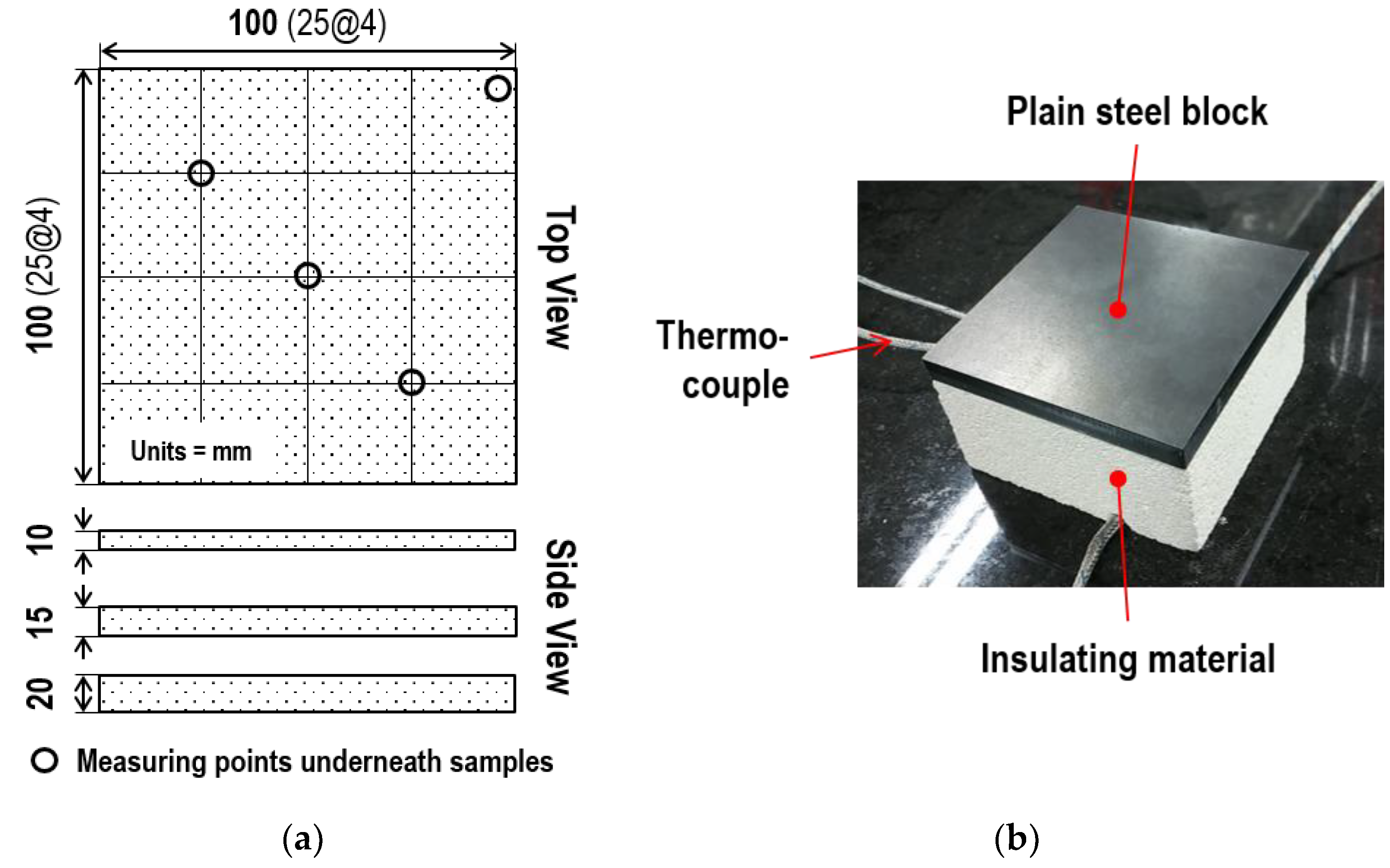
3. Experimental Details
4. Determination of Key Parameters
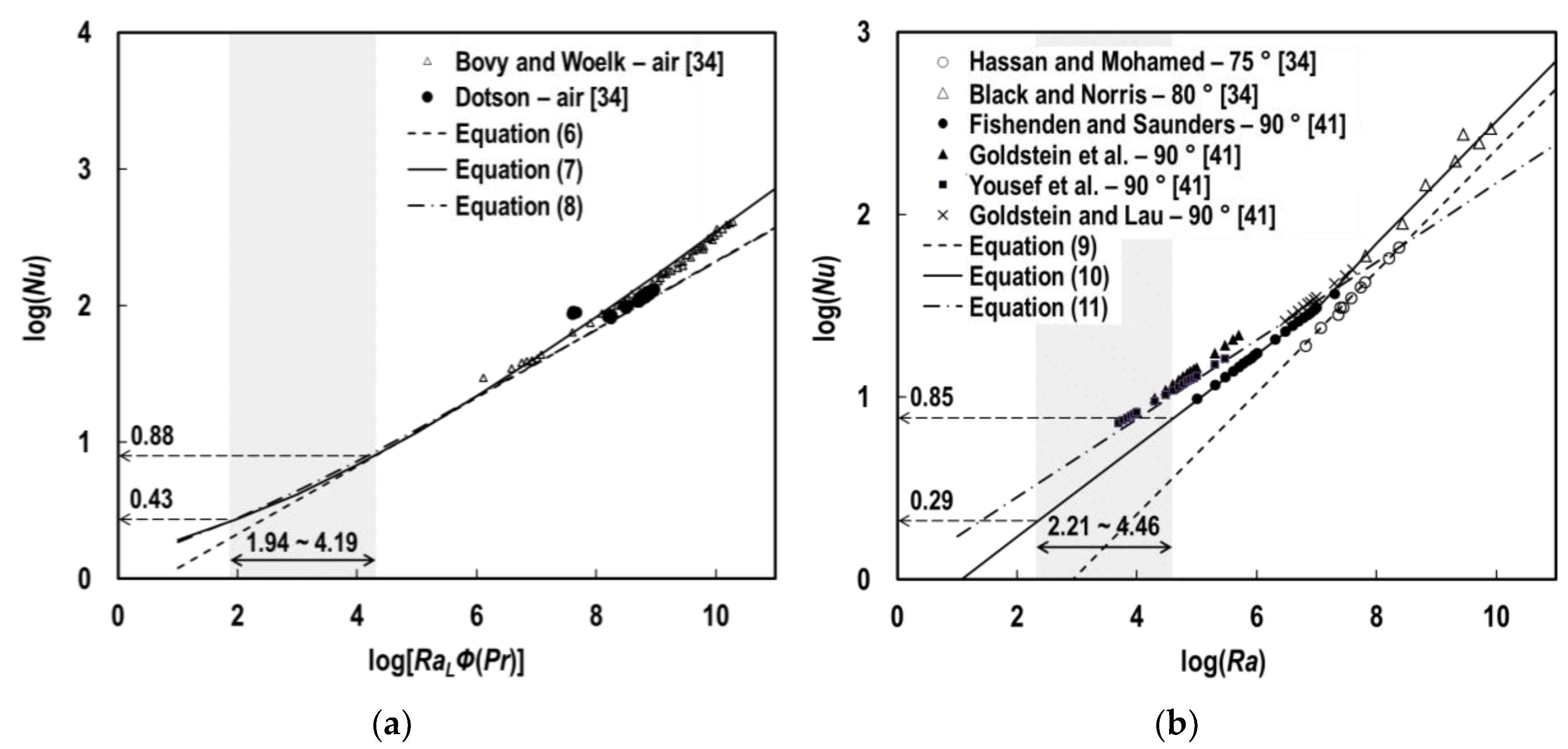
4.1. Convection Heat Transfer Coefficient
- In the tests, specimens’ exposed surfaces were heated consistently by a uniform radiant flux density emitted by the conical heater. Prior research [32,33] examined free convection from a vertical plane under such heating conditions, differentiated from the conventional condition for uniform wall temperatures, and developed a modified Rayleigh number. However, the deviations between the correlations obtained under the two different heating conditions are negligible in the case of free convective flow, adjacent to the vertical and horizontal planes [34]. Hence, the conventional version of the Rayleigh number, which has been more widely examined, was adopted for the steel block model studied in this work.
- Regarding surface orientation, the use of gravitational term in place of the gravitational acceleration ( in m/s2) in the typical Grashof number (Gr) was suggested for inclined surfaces, including horizontal surfaces [35], where θ is the angle of inclination from vertical in radians. This approach was capable of correlating well with the classical studies on free convective motion adjacent to vertical planes [36]. However, the correlations were not satisfactory for the horizontal top surface of the heated blocks [37], and even the turbulence data in this orientation from the air provide a closer correlation to the general than with the modified [34]. Considering these assertions, the conventional was adopted for the convection on the top surface of solids in this work.
- With respect to the flow regime, the onset of the transition in free convection over vertical planes occurs when is in the order of [38]. For inclined, upward-facing planes under uniform heat fluxes, a correlation for the critical was derived to be [39]. According to these suggestions, the patterns of fluid motions anticipated in this instrument were evaluated as laminar and turbulent for the side and top surfaces of the heated steel bodies, respectively.
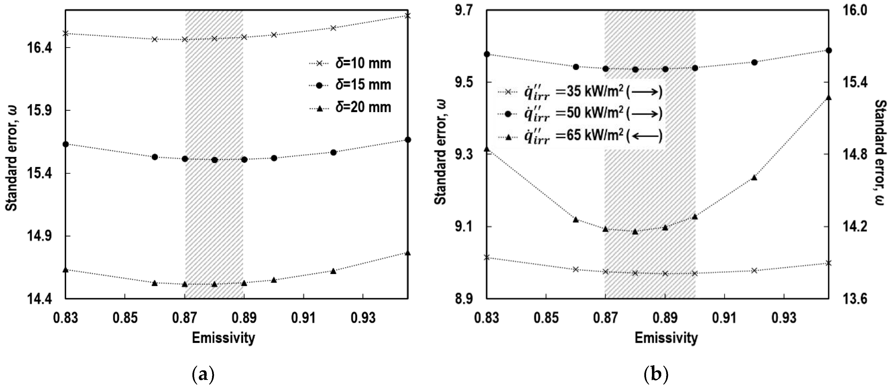
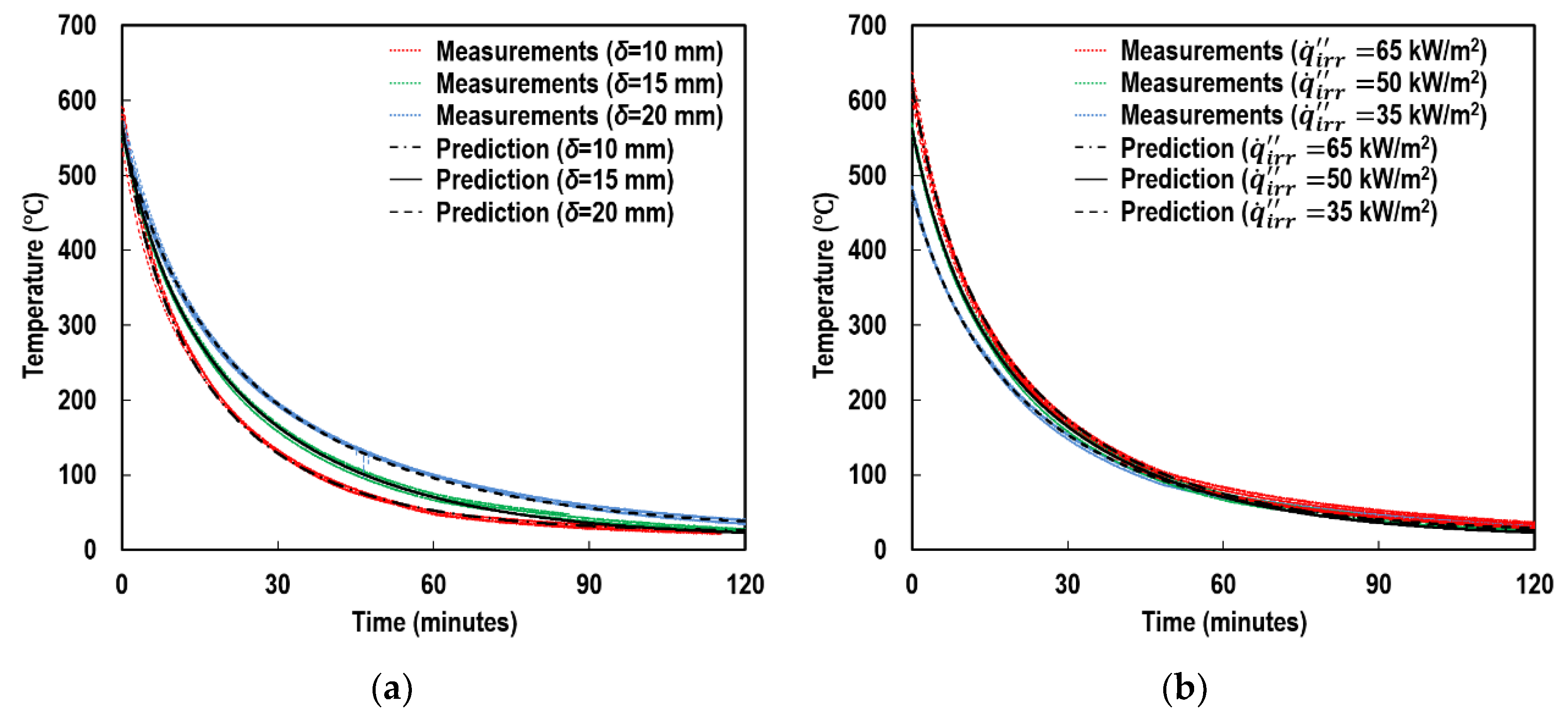
4.2. Emissivity
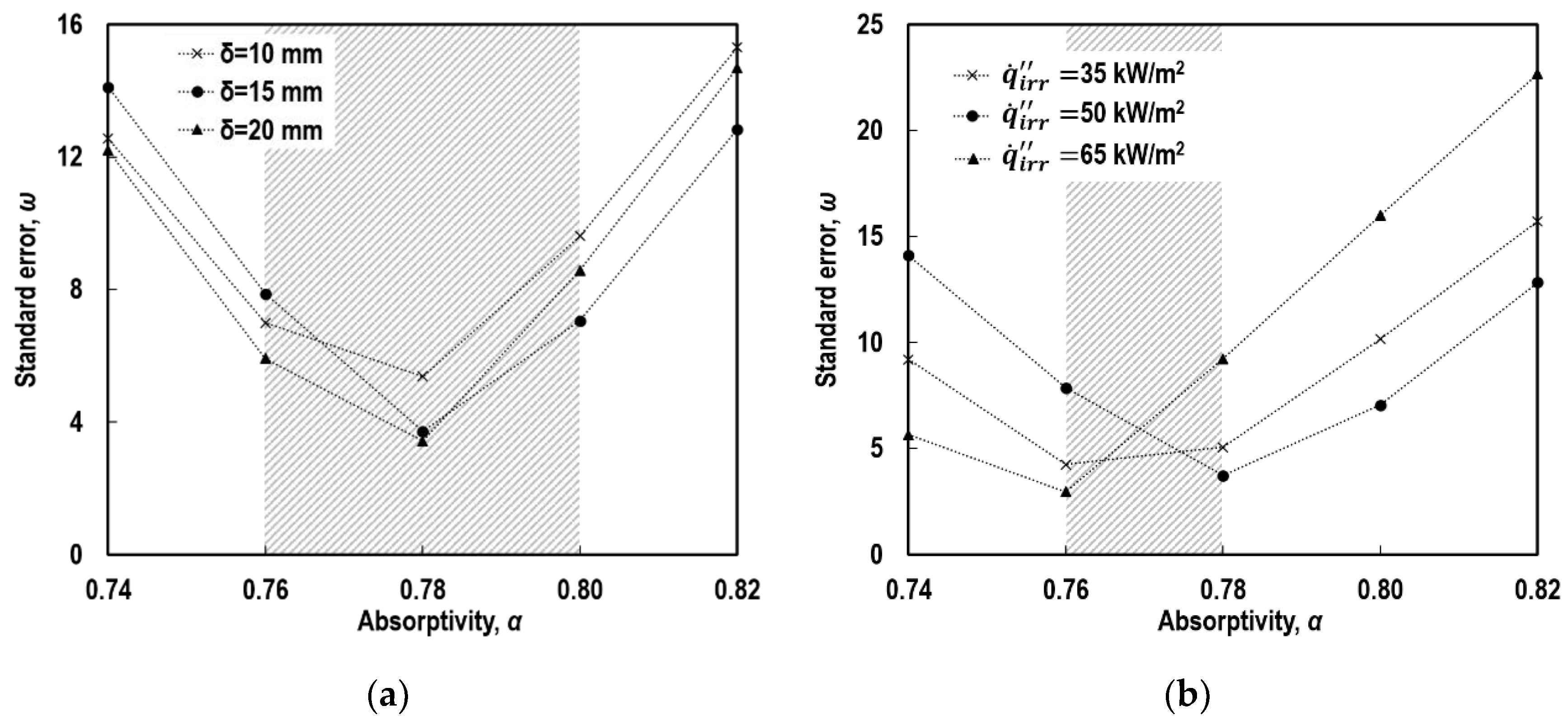
4.3. Absorptivity
5. Discussion
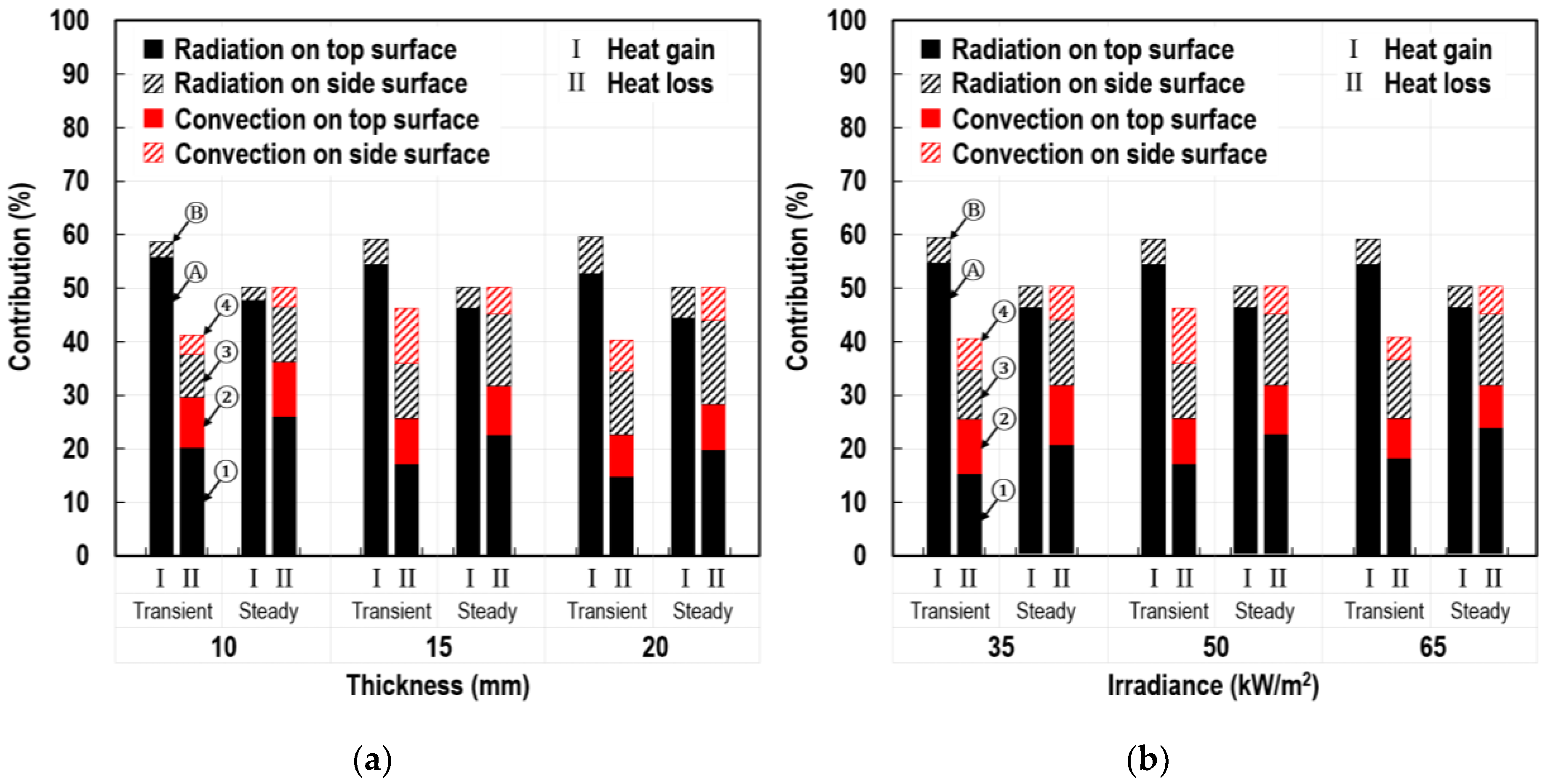
5.1. Individual Contributions of Top and Side Surfaces
5.2. Individual Contributions of Radiation and Convection Modes
5.3. Individual Contributions of Radiant Absorption and Emission
6. Conclusions
Author Contributions
Funding
Conflicts of Interest
References
- Janssens, M. Calorimetry (Chapter 27). In SFPE Handbook of Fire Protection Engineering, 5th ed.; Springer: New York, NY, USA, 2016. [Google Scholar]
- Babrauskas, V. The cone calorimeter (Chapter28). In SFPE Handbook of Fire Protection Engineering, 5th ed.; Springer: New York, NY, USA, 2016. [Google Scholar]
- Bartholmai, M.; Schriever, R.; Schartel, B. Influence of external heat flux and coating thickness on the thermal insulation properties of two different intumescent coatings using cone calorimeter and numerical analysis. Fire Mater. 2003, 27, 151–162. [Google Scholar] [CrossRef]
- Zhang, J.; Delichatsios, M.A. Determination of the convective heat transfer coefficient in three-dimensional inverse heat conduction problems. Fire Saf. J. 2009, 44, 681–690. [Google Scholar] [CrossRef]
- Griffin, G.J. The modelling of heat transfer across intumescent polymer coatings. J. Fire Sci. 2010, 28, 249–277. [Google Scholar] [CrossRef]
- Zhang, Y.; Wang, Y.C.; Bailey, C.G.; Taylor, A.P. Global modelling of fire protection performance of intumescent coating under different cone calorimeter heating conditions. Fire Saf. J. 2012, 50, 51–62. [Google Scholar] [CrossRef]
- Wang, Y.; Göransson, U.; Holmstedt, G.; Omrane, A. A model for prediction of temperature in steel structure protected by intumescent coating, based on tests in the cone calorimeter. Fire Saf. Sci. 2005, 8, 235–246. [Google Scholar] [CrossRef]
- Mesquita, L.M.R.; Piloto, P.A.G.; Vaz, M.A.P.; Pinto, T.M.G. Decomposition of intumescent coatings: Comparison between a numerical method and experimental results. Acta Polytech. 2009, 49, 60–65. [Google Scholar]
- Han, Z.; Fina, A.; Malucelli, G.; Camino, G. Testing fire protective properties of intumescent coatings by in-line temperature measurements on a cone calorimeter. Prog. Org. Coat. 2010, 69, 475–480. [Google Scholar] [CrossRef]
- Kang, S.; Choi, S.; Choi, J.Y. View factor in cone calorimeter testing. Int. J. Heat Mass Transf. 2016, 93, 217–227. [Google Scholar] [CrossRef]
- Kang, S.; Choi, S.; Choi, J.Y. Numerical prediction on interacting thermal-structural behaviour of inorganic intumescent coating. In Proceedings of the International Conference and Exhibition on Fire Science and Engineering (Interflam), Nr Windsor, UK, 4–6 July 2016; pp. 213–224. [Google Scholar]
- Kang, S.; Choi, S.; Choi, J.Y. Mechanism of heat transfer through porous media of inorganic intumescent coating in cone calorimeter testing. Polymers 2019, 11, 221. [Google Scholar] [CrossRef] [PubMed]
- Kang, S.; Choi, S.; Choi, J.Y. Coupled thermos-physical behaviour of an inorganic intumescent system in cone calorimeter testing. J. Fire Sci. 2017, 35, 207–234. [Google Scholar] [CrossRef]
- Wilson, M.T.; Dlugogorski, B.Z.; Kennedy, E.M. Uniformity of radiant heat fluxes in cone calorimeter. Fire Saf. Sci. 2003, 7, 815–826. [Google Scholar] [CrossRef]
- Siegel, R.; Howell, J.R. Thermal Radiation Heat Transfer, 4th ed.; Taylor & Francis: London, UK, 2002. [Google Scholar]
- Rhodes, B.T.; Quintiere, J.G. Burning rate and flame heat flux for PMMA in a cone calorimeter. Fire Saf. J. 1996, 26, 221–240. [Google Scholar] [CrossRef]
- Hopkins, D.; Quintiere, J.G. Material fire properties and predictions for thermoplastics. Fire Saf. J. 1996, 26, 241–268. [Google Scholar] [CrossRef]
- Janssens, M. A thermal model for piloted ignition of wood including variable thermophysical properties. Fire Saf. Sci. 1991, 3, 167–176. [Google Scholar] [CrossRef]
- Janssens, M.L. Improved method for analysing ignition data from the Cone Calorimeter in the vertical orientation. Fire Saf. Sci. 2003, 7, 803–814. [Google Scholar] [CrossRef]
- Staggs, J.E.J. Convection heat transfer in the cone calorimeter. Fire Saf. J. 2009, 44, 469–474. [Google Scholar] [CrossRef]
- de Ris, J.L.; Khan, M.M. A sample holder for determining material properties. Fire Mater. 2000, 24, 219–226. [Google Scholar] [CrossRef]
- Lautenberger, C.; Rein, G.; Fernandez-Pello, C. The application of a genetic algorithm to estimate material properties for fire modelling from bench-scale fire test data. Fire Saf. J. 2006, 41, 204–214. [Google Scholar] [CrossRef]
- Modest, M.F. Radiative Heat Transfer, 2nd ed.; Academic Press: London, UK, 2003. [Google Scholar]
- Bergström, D. The Absorption of Laser Light by Rough Metal Surfaces. Ph.D. Thesis, Lulea University of Technology, Lulea, Sweden, June 2008. [Google Scholar]
- Furber, B.N.; Broderick, R. The development of an apparatus to measure the normal emissivity of small plane samples in a controlled atmosphere. SAGE J. 1967, 182, 120–129. [Google Scholar] [CrossRef]
- Boyden, S.; Zhang, Y. Temperature and wavelength-dependent spectral absorptivities of metallic materials in the infrared. J. Thermophys. Heat Transf. 2006, 20, 9–15. [Google Scholar] [CrossRef]
- Paloposki, T.; Liedquist, L. NT technical report 570. In Steel Emissivity at High Temperatures; VTT: Espoo, Finland, 2006. [Google Scholar]
- Wen, C.D. Investigation of steel emissivity behaviours: Examination of Multispectral Radiation Thermometry (MRT) emissivity models. Int. J. Heat Mass Transf. 2010, 53, 2035–2043. [Google Scholar] [CrossRef]
- Försth, M.; Roos, A. Absorptivity and its dependence on heat source temperature and degree of thermal breakdown. Fire Mater. 2011, 35, 285–301. [Google Scholar] [CrossRef]
- Kays, W.M.; Crawford, M.E. Free-convection boundary layers. In Convective Heat and Mass Transfer, 3rd ed.; McGraw-Hill Inc.: New York, NY, USA, 1993. [Google Scholar]
- Çengel, Y.A. Heat and Mass Transfer-A Practical Approach, 3rd ed.; McGraw-Hill Inc.: New York, NY, USA, 2007. [Google Scholar]
- Sparrow, E.M.; Gregg, J.L. Laminar free convection from a vertical plate with uniform surface heat flux. Trans. ASME 1956, 78, 435–440. [Google Scholar]
- Churchill, S.W.; Chu, H.H.S. Correlating equations for laminar and turbulent free convection from a vertical plate. Int. J. Heat Mass. Transf. 1975, 18, 1323–1329. [Google Scholar] [CrossRef]
- Churchill, S.W. Heat exchanger theory. In Heat Exchanger Design Handbook; Hemisphere Publishing Corporation: Washington, DC, USA, 1983; pp. 2.5.7-1–2.5.7-31. [Google Scholar]
- Rich, B.R. An investigation of heat transfer from an inclined flat plate in free convection. Trans. ASME 1953, 75, 489. [Google Scholar]
- Lloyd, J.R.; Sparrow, E.M.; Eckert, E.R.G. Laminar, transition and turbulent natural convection adjacent to inclined and vertical surfaces. Int. J. Heat Mass Transf. 1972, 15, 457–473. [Google Scholar] [CrossRef]
- Bergman, T.L.; Lavine, A.S.; Incropera, F.P.; DeWitt, D.P. Fundamentals of Heat and Mass Transfer, 7th ed.; John Wiley & Sons: Hoboken, NJ, USA, 2011. [Google Scholar]
- Klyacho, L.S. Relations for the critical state describing transition from laminar to turbulent flow in free convection. Int. J. Heat Mass Transf. 1962, 5, 763–764. [Google Scholar] [CrossRef]
- Fussey, D.E.; Warneford, I.P. Free convection from a downward facing inclined flat plate. Int. J. Heat Mass Transf. 1978, 21, 119–216. [Google Scholar] [CrossRef]
- Churchill, S.W.; Ozoe, H. A correlation for laminar free convection from a vertical plate. ASME J. Heat Transf. 1973, 95, 540–541. [Google Scholar] [CrossRef]
- Corcione, M. Heat transfer correlations for free convection from upward-facing horizontal rectangular surfaces. WSEAS Trans. Heat Mass Transf. 2007, 2, 48–60. [Google Scholar]
- KS D3515:2014. Rolled Steels for Welded Structures; Korean Industrial Standard; Korean Agency for Technology and Standards: Chungcheongbuk-do, Korea, 2013.
- Hyundai Steel, Products Guide. Available online: https://www.hyundai-steel.com/kr/down/ProductsGuide.pdf (accessed on 7 July 2019).
- Touloukian, Y.S.; DeWitt, D.P. Thermal Radiative Properties: Metallic Elements and Alloys; IFI/Plenum: New York, NY, USA; Washington, DC, USA, 1970; Volume 7. [Google Scholar]
- BS EN 1993-1-2 Eurocode 3: Design of Steel Structures—Part 1-2: General Rules—Structural Fire Design; European Committee for Standardization: Brussels, Belgium, 2005.


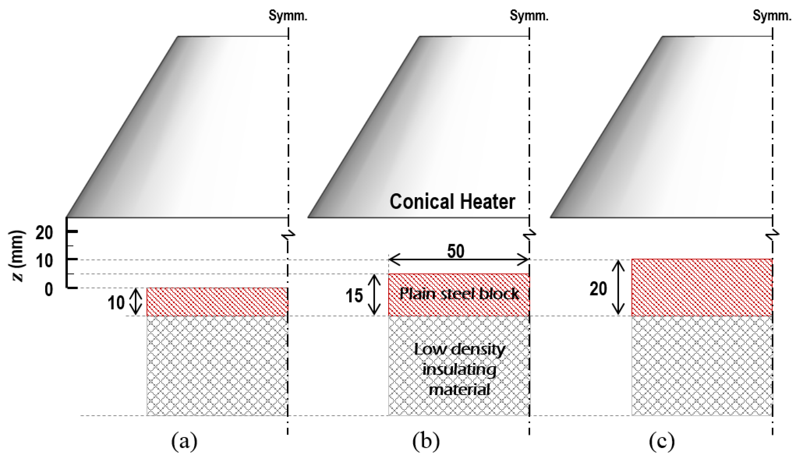
| H a (mm) | Thickness of Specimens δ (mm) | View Factor | |
|---|---|---|---|
| Top Surface b (Fh-top) | Side Surface c (Fh-side) | ||
| 25 | 10 | 0.2508 | 0.0151 |
| 20 | 15 | 0.2627 | 0.0263 |
| 15 | 20 | 0.2730 | 0.0410 |
| Author | Convection Heat Transfer Coefficient (W/m2K) |
|---|---|
| Janssens (1991) | 9–27 a |
| Rhodes et al. (1996) | 10 |
| Hopkins Jr. et al. (1996) | 10 |
| de Ris et al. (2000) | 7.6 |
| Janssens (2002) | 3.9–17.1 a |
| Bartholmai et al. (2003) | 20 |
| Wang (2005) | 20 |
| Lautenberger et al. (2006) | 10 |
| Staggs (2009) | 15.15–25.25 |
| Zhang et al. (2009) | 7–15 |
| Mesquita et al. (2009) | 20 |
© 2019 by the authors. Licensee MDPI, Basel, Switzerland. This article is an open access article distributed under the terms and conditions of the Creative Commons Attribution (CC BY) license (http://creativecommons.org/licenses/by/4.0/).
Share and Cite
Kang, S.; Kwon, M.; Choi, J.Y.; Choi, S. Thermal Boundaries in Cone Calorimetry Testing. Coatings 2019, 9, 629. https://doi.org/10.3390/coatings9100629
Kang S, Kwon M, Choi JY, Choi S. Thermal Boundaries in Cone Calorimetry Testing. Coatings. 2019; 9(10):629. https://doi.org/10.3390/coatings9100629
Chicago/Turabian StyleKang, Sungwook, Minjae Kwon, Joung Yoon Choi, and Sengkwan Choi. 2019. "Thermal Boundaries in Cone Calorimetry Testing" Coatings 9, no. 10: 629. https://doi.org/10.3390/coatings9100629
APA StyleKang, S., Kwon, M., Choi, J. Y., & Choi, S. (2019). Thermal Boundaries in Cone Calorimetry Testing. Coatings, 9(10), 629. https://doi.org/10.3390/coatings9100629