Abstract
The shape, size, and interfacial transition zone (ITZ) of aggregates significantly impact the nonlinear mechanical behavior of concrete. This study investigates concrete’s mechanical response and damage mechanisms by developing a three-dimensional, three-phase mesoscale model comprising coarse aggregates, mortar, and ITZ to explore the compressive performance of concrete. A method for simulating the random distribution of aggregates based on three-dimensional grid partitioning is proposed, where the value of each grid point represents the maximum aggregate radius that can be accommodated if the point serves as the aggregate center. Aggregates are generated by randomly selecting grid points that meet specific conditions, avoiding overlapping distributions and significantly improving computational efficiency as the generation progresses. This model effectively enhances the precision and efficiency of aggregate distribution and provides a reliable tool for studying the random distribution characteristics of aggregates in concrete. Additionally, an efficient discrete element model (DEM) was established based on this mesoscale model to simulate the compressive behavior of concrete, including failure modes and stress–strain curves. The effects of aggregate shape and maximum aggregate size on the uniaxial compressive failure behavior of concrete specimens were investigated. Aggregate shape has a particular influence on the compressive strength of concrete, and the compressive strength decreases with an increase in maximum aggregate size. Combined with existing experimental results, the proposed mesoscale model demonstrates high reliability in analyzing the compressive performance of concrete, providing valuable insights for further research on the mechanical properties of concrete.
1. Introduction
Concrete is a typical heterogeneous multiphase composite material composed of coarse aggregates, mortar, and the interfacial transition zone (ITZ) between them. Due to its excellent mechanical properties, durability, and engineering adaptability, concrete is widely used in various civil engineering applications [1,2,3]. However, significant physical and mechanical differences exist among the internal components of concrete, especially regarding the geometry, size distribution, and spatial arrangement of aggregates, which greatly influence the overall mechanical response and failure mechanism of concrete [4,5]. Therefore, accurately characterizing the spatial distribution of aggregates and conducting multiscale mechanical behavior analysis based on this is key to understanding the nonlinear mechanical properties of concrete materials. Mesoscale numerical simulation of concrete holds significant theoretical and practical importance [6].
In recent years, with the continuous advancement of computational mechanics and material modeling technologies, mesoscale numerical simulation methods have received widespread attention in the mechanical study of concrete [7,8,9]. Particularly at the two-dimensional (2D) level, various random aggregate generation methods have been proposed, such as the Monte Carlo method, digital image-based techniques, and Voronoi diagram-based algorithms [10,11,12,13]. These approaches have achieved notable progress in simulating aggregate shape, size distribution, and spatial occupation characteristics, thereby supporting 2D mesoscale mechanical analyses to a certain extent. The Voronoi-based methods enable the generation of polygonal aggregates resembling real shapes observed in concrete sections [10], while digital image methods can reconstruct actual microstructures from thin-section images or CT scans [11], thus ensuring more accurate spatial distributions. Monte Carlo simulations provide a statistical framework for controlling gradation and area fractions [12]. However, due to the inherent limitations of 2D models in representing the actual spatial distribution and mechanical interactions of aggregates, they are unable to accurately capture the complex three-dimensional (3D) behavior of aggregates and the propagation paths of cracks. This restricts their applicability in realistically simulating the failure processes of concrete. Consequently, 3D mesoscale models have emerged as essential tools for investigating the heterogeneous properties and failure mechanisms of concrete. In 3D models, coarse aggregates, mortar, and ITZ are typically treated as separate physical phases. By accurately simulating their geometrical configurations, mechanical properties, and interactions, these models enable more realistic predictions of concrete’s mechanical response and damage evolution under loading.
Although three-dimensional mesoscale modeling can more realistically reflect the internal structure and mechanical response of concrete, the generation of randomly distributed aggregates in 3D still faces numerous challenges [3,14,15,16]. Existing studies mainly adopt the following types of methods for 3D aggregate modeling: (1) sphere packing methods, which achieve aggregate filling by controlling the particle size distribution and enforcing non-overlapping constraints [17,18]; (2) image reconstruction-based 3D visualization techniques, such as CT image reconstruction or digital voxel models, which are suitable for simulating realistic aggregate morphologies [19,20]; and (3) geometric modeling methods based on mathematical shape descriptions (e.g., polyhedra, ellipsoids) to approximate the actual shape of aggregates [8,21,22]. The work of Yang and Wang [17] introduced an improved dynamic packing algorithm for polydisperse spherical particles, significantly enhancing packing efficiency. Wang et al. [19] used high-resolution CT scanning and segmentation algorithms to extract realistic 3D aggregate shapes, which were then meshed for finite element analysis. These methods each have their strengths and weaknesses in terms of modeling accuracy, but they commonly suffer from high computational costs, low modeling efficiency, and difficulties in overlap control—issues that become particularly significant in large-scale or high-volume-fraction simulations. Furthermore, to ensure the stability and convergence of subsequent numerical simulations, the aggregate generation process must balance spatial uniformity and physical realism, which further increases the complexity of modeling. Therefore, achieving efficient and automated 3D aggregate generation and model construction while maintaining physical realism remains one of the key challenges in the current field of mesoscale concrete modeling.
Based on the development of three-dimensional mesoscale models, researchers have gradually applied them to analyze the mechanical behavior of concrete, particularly in studying crack evolution, failure mechanisms, and strength prediction [23,24,25,26]. Common approaches include the finite element method (FEM), finite difference method (FDM), and phase-field method, which, under the assumption of continuum mechanics, can effectively simulate internal stress distributions and macroscopic responses [27,28,29,30]. However, concrete is inherently a discontinuous and heterogeneous material, and its failure process often involves particle-level cracking, sliding, and rearrangement. Therefore, traditional continuum-based methods exhibit limitations in capturing nonlinear failure behavior. For instance, crack paths cannot naturally emerge, local stress concentrations may lead to numerical instability, and it remains difficult to accurately model damage evolution in the ITZ region—especially in post-peak and large-deformation stages. Continuum-based FEM tends to smear cracks and underestimate strain localization [28], whereas the incorporation of discontinuity-enhanced formulations has been emphasized to better capture crack initiation and branching [29]. To overcome these limitations, increasing attention has been given to the discrete element method (DEM) for modeling and analyzing the mesoscale structure of concrete [31,32,33]. DEM treats the material as an assembly of rigid or elastic particles, and by defining contact interactions between particles, it can explicitly simulate crack initiation, propagation, and coalescence, making it inherently suitable for modeling discontinuous failure processes. Moreover, DEM excels in handling large deformations, particle interactions, and nonlinear mechanical properties, making it particularly effective in studying the influence of aggregate shape, interface strength, and particle distribution on overall mechanical performance. Therefore, integrating DEM into an efficient 3D aggregate generation method holds great potential for significantly improving the accuracy and stability of concrete mechanical simulations and provides a robust numerical tool for uncovering failure mechanisms and guiding structural design optimization.
Over the last decade, the typical take-and-place method involving overlap detection has become well developed [34,35,36,37,38]. Despite substantial efforts to improve the efficiency of aggregate placement, overlap detection remains complex and time-consuming, especially in 3D cases. As described in the recent literature, conventional 2D random aggregate concrete samples generated using this method require several hours, while 3D methods may take dozens of hours [35,36,37,38]. This study addresses some challenges associated with traditional methods for generating random aggregates in concrete and proposes a novel algorithm with significant advantages. Traditional methods typically require constant calculation of the distance relationships between newly generated aggregates and existing ones. As more aggregates are generated, the algorithm may become redundant, leading to a significant decline in efficiency, mainly when dealing with densely packed composite materials. The random aggregate generation algorithm proposed in this study performs exceptionally well in addressing these issues. The main advantage of this algorithm is that the speed of generating individual new aggregates gradually increases as the number of aggregates grows. By employing an innovative approach, the occupied regions of already-generated aggregates are excluded from subsequent calculations for new aggregates, effectively avoiding overlaps between newly generated and existing aggregates. This strategy ensures that the overall generated aggregates remain non-overlapping and significantly enhances computational efficiency. The effectiveness of this method was validated through discrete element numerical simulations and physical experiments. Additionally, the study investigated the effects of aggregate shape and particle size on the uniaxial compressive strength of concrete specimens.
2. Materials and Methods
Herein, this paper proposes a method for generating randomly distributed irregular concrete aggregates, including a 3D grid partitioning method, a random ellipsoid generation method, an irregular polyhedron generation method, an optimization method for irregular polyhedra, and a method for generating ITZs.
2.1. Three-Dimensional Grid Partitioning
This paper proposes an original method for partitioning 3D meshes [39,40]. The method calculates a value d for each mesh, where d can be interpreted as the radius of the most enormous inscribed sphere. The core of the method involves dividing the unoccupied regions into 3D meshes and assigning values to all mesh regions. The maximum value, dmax, represents the radius of the most enormous inscribed sphere, and the major axis of the generated aggregate is constrained not to exceed dmax. After generating new aggregates, the mesh values for regions not occupied by aggregates must be recalculated.
The specific steps are as follows: We assume the entire computational domain initially consists of cement mortar before the first aggregate generation. A boundary layer is added around the computational domain to serve as the boundary conditions, and its value is set to 0. For each cement mortar mesh, the d-value is calculated. All cement mortar meshes are initialized with d = 0.5. If all meshes within a distance of d + 0.5 from a given cement mortar mesh also consist of cement mortar, the d-value is incremented by 0.5; otherwise, the d-value remains unchanged. This process is repeated until d-values for all cement mortar meshes are calculated, resulting in the distribution of d-values across the computational domain. The specific process is illustrated in Figure 1, and Figure 2 presents d-value distributions for some simple meshes.
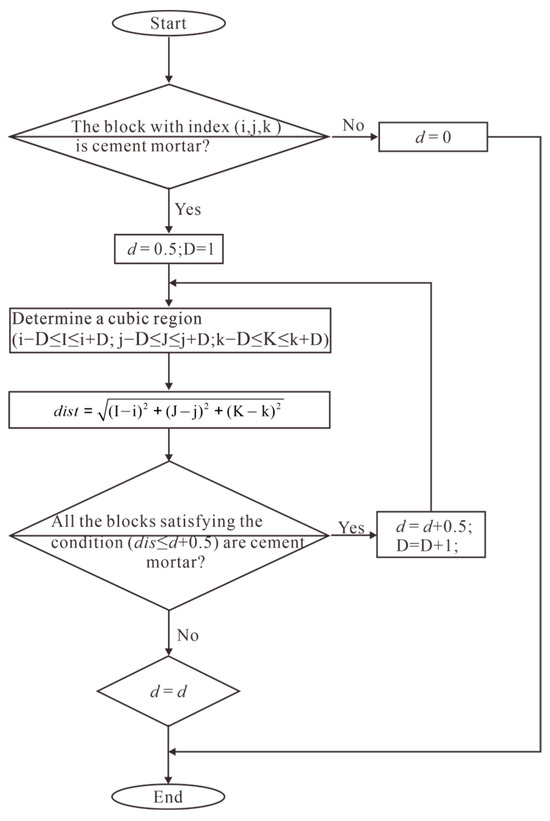
Figure 1.
Flowchart of d-value distribution. D represents half the side length of the cubic computational domain. I, J, and K denote the coordinates of the small cubes within the computational domain in the x, y, and z directions, respectively.
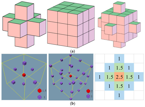
Figure 2.
Simple cement mortar model and d-value distribution: (a) schematic diagram of a simple model, (b) d-value distribution map, where different colors represent the corresponding d-values of each grid element shown in (a).
2.2. Arbitrary Distribution Ellipsoid Generation Method
This paper adopts an aggregate generation strategy of first placing large-sized aggregates, followed by small-sized aggregates. This approach better fills the gaps between coarse aggregates, enhancing the compactness of the concrete. It ensures a uniform distribution of all components in the concrete, thereby improving its workability and performance. The subsequent addition of small-sized aggregates further fills the voids, reducing the porosity and enhancing the compactness and durability of the concrete.
The maximum value in the d-value distribution corresponds to the maximum length of the ellipsoid’s major axis. Ellipsoids with larger major axes are generated first to achieve a more reasonable random aggregate distribution. Regions where the d-value is greater than or equal to a are identified. These regions can accommodate the ellipsoid. The center point and orientation angle of the ellipsoid are randomly selected within these regions. The parametric equation of the ellipsoid in spherical coordinates is
where (rx, ry, rz) are the coordinates of the ellipsoid’s center. a, b, and c are the semi-axis lengths of the ellipsoid along the three coordinate axes. θ is the polar angle, and ϕ is the azimuthal angle.
The rotation matrices Rx, Ry, and Rz are obtained by rotating around the x, y, and z axes, respectively. They are represented as follows:
The overall rotation matrix is
The coordinates of any point (x, y, z) inside the ellipsoid are transformed into new coordinates after being rotated by the rotation matrix R. The specific expression is as follows:
2.3. Generation Method for Irregular Polyhedra
One of the most frequently occurring sequences in nature is the Fibonacci sequence. With further exploration, it was discovered that this sequence leads to the golden ratio [41,42]. The Golden Section Spiral method has been widely applied and validated in science and engineering, demonstrating a strong theoretical foundation and practical effectiveness. Due to its ability to generate points with excellent uniformity and distribution properties, the Golden Section Spiral method is extensively used in computer graphics, scientific computation, and materials science. Its solid theoretical basis has been verified and applied in numerous studies.
The Golden Section Spiral method is highly extensible and can generate points on spheres, ellipsoids, and other geometric shapes. Its application is not limited to specific geometries. Simple yet effective, this method can produce large-scale point sets with minimal computation, avoiding complex iterative or optimization processes. It is particularly adept at generating uniformly distributed points on spherical or ellipsoidal surfaces. Uniform distribution ensures equal intervals between points, avoiding clustering or sparse regions.
To prevent collinearity or coplanarity, this paper utilizes the Golden Section Spiral method to generate 2N uniformly distributed points on the surface of an ellipsoid. N points are randomly selected from these to construct irregular polyhedra, ensuring randomness in the polyhedron’s shape.
For the i-th point generated using the Golden Section Spiral method on the surface of the ellipsoid, its polar and azimuthal angles can be expressed as follows:
The expression for mapping points onto the surface of an ellipsoid is
This generates a 3D irregular aggregate (Figure 3) comprising 10 vertices.
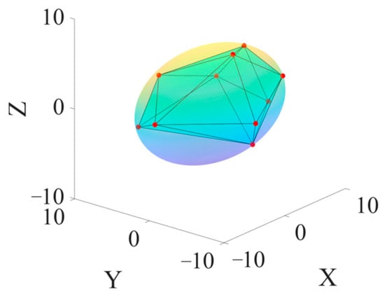
Figure 3.
Three-dimensional irregular aggregate.
2.4. Optimization of Irregular Polyhedra
Although the above method can generate irregular aggregates, the resulting aggregates require optimization before they can be used for numerical calculations. Three aspects of optimization are performed here: eliminating flatness, removing triangular faces with very short edges, and eliminating triangular faces with extremely small interior angles.
Flat polyhedra, especially those with complex shapes [43,44], may have overlapping vertices or edges. They may also have intersecting or overlapping faces on the same plane. Aggregates with very short edges can affect computational efficiency. Extremely small interior angles can also reduce simulation accuracy. This study further optimizes the generated aggregates to address this issue.
First, sphericity describes the degree of flatness to avoid obtaining flat-shaped aggregates. Sphericity B is defined as [45]
where Ll, Li, and Ls represent the longest, intermediate, and shortest particle dimensions, respectively. Considering that planar aggregates usually have very low sphericity, the minimum sphericity is set to 0.4. Therefore, only aggregates with a sphericity greater than 0.4 can be generated.
Next, edge length optimization is performed by calculating the length of each edge of the aggregate. If the shortest edge in a triangular face is smaller than the predefined minimum length Lmin, one of the vertices of that edge is removed (Figure 4). Lmin is set as one tenth of the aggregate’s maximum edge length. The new aggregate, defined by the remaining vertices, is further optimized until all edge lengths exceed Lmin.
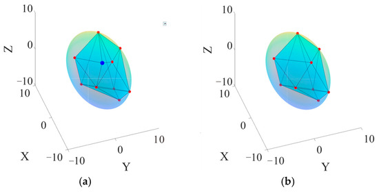
Figure 4.
Optimization of triangles with shortest edges: (a) aggregate before optimization; (b) aggregate after optimization. The blue dots represent the vertices to be removed, and the red dots indicate the vertices to be retained.
Finally, interior angle optimization is carried out by calculating the interior angles of each triangular face of the aggregate. If the smallest interior angle is less than the predefined value β (set to 10° here), the other two interior angles of the triangle are compared. The vertex corresponding to the larger interior angle is removed (Figure 5). The new aggregate, formed by the remaining vertices, undergoes further optimization until all interior angles exceed β. After the geometric optimization of all aggregates, the resulting aggregates are well-shaped and free from overlaps.
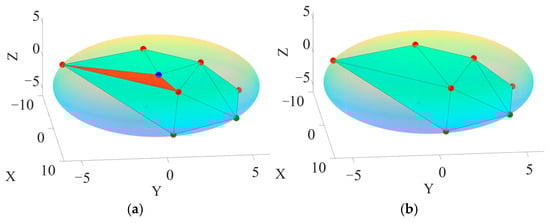
Figure 5.
Optimization of triangles with minimum interior angles: (a) aggregate before optimization; (b) aggregate after optimization. The blue dots represent the vertices to be removed, and the red dots indicate the vertices to be retained.
2.5. Generate Bonding Interface
First, calculate the centroid of the polyhedron. The centroid is the average of all vertex coordinates:
where represents the centroid coordinates, N is the number of vertices, and Xi, Yi, and Zi are the coordinates of the i-th vertex.
Next, calculate the distance di from each vertex to the centroid:
Assuming the thickness of the bonding interface is l, the distance from the shrunken new vertex to the centroid is
The coordinates of the new shrunken vertex are
Figure 6 shows the bonding interface constructed in this study. In the figure, the red points represent the original vertices of the irregular polyhedron randomly selected on the ellipsoidal surface. In contrast, the blue points represent the vertices of the shrunken irregular polyhedron. The region between the two polyhedra constitutes the bonding interface. Since the bonding interface is generated using a shrinking method, DD = H + 2l, ensuring sufficient space for the generation of aggregates and the bonding interface. Figure 7 illustrates the flowchart for generating three-dimensional randomly distributed irregular aggregates. Figure 8 displays the three-dimensional randomly distributed irregular aggregates, with different colors representing aggregates of different particle sizes.
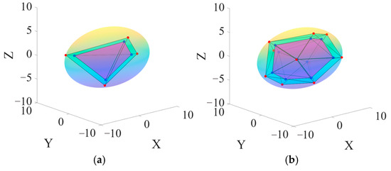
Figure 6.
Schematic diagram of the 3D bonding interface: (a) randomly select 4 points; (b) randomly select 10 points. Red points are the original polyhedron vertices on the ellipsoidal surface, and blue points are the vertices of the shrunken polyhedron. The bonding interface lies between the two polyhedra.
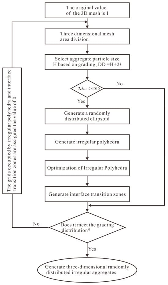
Figure 7.
Flowchart for generating 3D randomly distributed irregular aggregates. dmax represents the maximum value after dividing the 3D grid region, and l represents the thickness of the bonding interface.
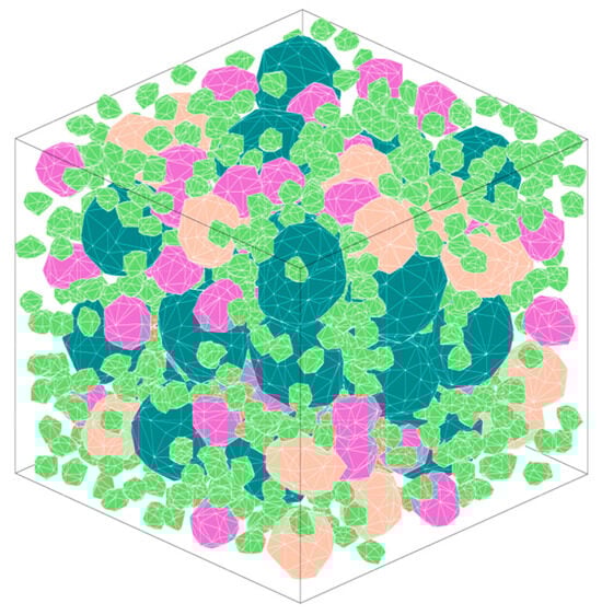
Figure 8.
Three-dimensional randomly distributed irregular aggregates. Different colors represent aggregates of different particle sizes.
In traditional methods for generating 3D random aggregates, the spatial relationship between a new aggregate and the existing aggregates must be determined [36,46]. As the number of generated aggregates increases, the time required to generate new aggregates also grows. The random aggregate generation model proposed in this study adopts a three-dimensional grid partitioning method. Each grid cell’s value represents the maximum aggregate radius that can be accommodated if the grid point is used as the aggregate center. By randomly selecting grid points that meet the conditions, aggregates are generated, ensuring a reasonable distribution of aggregates. The innovation of the model lies in the fact that when a new aggregate is generated, the regions occupied by existing aggregates are excluded from further grid partitioning. This approach avoids overlap between new and existing aggregates and significantly reduces the time required to generate new aggregates as the number of aggregates increases. Twenty irregular aggregates with a particle size of 20 mm are randomly generated within a model of dimensions 75 mm × 75 mm × 75 mm (Figure 9). Figure 10 shows the time required to generate each aggregate. The figure indicates that as the number of generated aggregates increases, the time required to generate new aggregates decreases, with a noticeable reduction in the time required for the initial stages of aggregate generation.
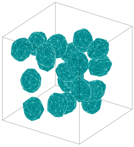
Figure 9.
Randomly distributed irregular aggregates of the same size.
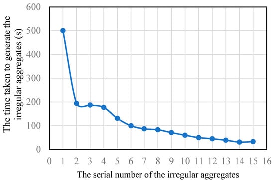
Figure 10.
The time taken to generate irregular aggregates of the same size.
3. Discrete Element Method
The particle flow method is founded on Newton’s second law and the force–displacement law. The computational process revolves around two core iterative steps: applying Newton’s second law to particle elements and applying the force–displacement law to contact points. Newton’s second law primarily determines each particle element’s motion state and updates its state variables accordingly. The force–displacement law updates contact state variables based on the relative motion at each contact point, thereby updating contact forces, as illustrated in Figure 11.
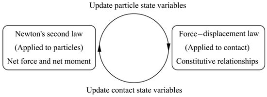
Figure 11.
Diagram of the PFC computational iteration process.
Additionally, Newton’s second law does not apply to the movement of walls, as their motion is generally predefined. In PFC simulations, the force–displacement law only considers the contact interactions between particle elements and walls during calculations.
3.1. Force–Displacement Law
The force–displacement law is central to the computational process of PFC simulations. By introducing the normal stiffness and tangential stiffness parameters, PFC effectively resolves the relationship between force and displacement for two contacting elements. The normal vector of the contacting elements determines the exact position of the contact point. In particle flow simulations, the contact forms are mainly categorized into “particle–particle” and “particle–wall” interactions, both crucial for describing the dynamic behavior of the particle flow system, as shown in Figure 12. In this figure, , represents the radii of the particles, and denote the centers of the particles, stands for the center of rotation and displacement of the wall, and indicates the distance between two elements. When is negative, it signifies the contact amount (or overlap), denoted as .
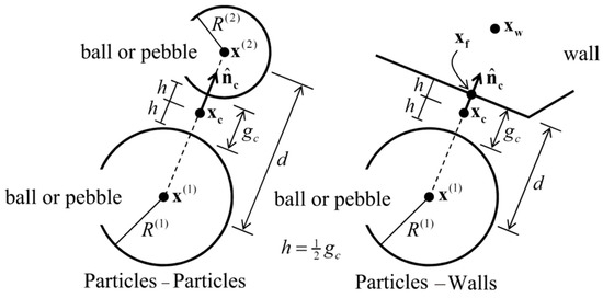
Figure 12.
Forms of element contact.
In applying the force–displacement law to specific calculations, the contact force between two elements is divided into normal and tangential components. The normal force is proportional to the overlap amount, denoted as
where is the normal force, is the normal stiffness, and is the overlap amount.
The tangential force calculation is more complex due to its dependence on the motion and loading history of the particle elements. It is usually expressed in incremental form. When the relative displacement between two entities is , the incremental tangential force at the i-th time step can be expressed as
where is the incremental tangential force at the i-th step and is the tangential stiffness.
Considering the tangential force from the previous time step, the total tangential force is given by
These equations can be used to calculate the total contact force and contact moment of the contact elements in each computational time step.
3.2. Laws of Motion
In the particle flow model, the motion of particle elements is determined by the forces and moments acting on them. These forces and moments reflect the overall motion through the particle’s linear and angular velocities. The motion equations for particles consist of two main components: the linear motion equation, resulting from the net force, and the rotational motion equation, resulting from the net moment.
The linear motion equation is expressed as
where , , and are the net forces in the x, y, and z directions, respectively; represents the mass of the particle; , , and are the accelerations in the x, y, and z directions, respectively; and denotes gravitational acceleration.
The rotational motion equation is expressed as
where Mx, My, and Mz represent the net moments in the x, y, and z directions, respectively; Ixx, Iyy, and Izz are the elements of the inertia matrix; and ax, ay, and az are the angular accelerations in the x, y, and z directions, respectively.
3.3. Constitutive Models in PFC
In PFC, the description of macroscopic material constitutive properties relies on the definition of particle micro-contact models and their parameters. PFC includes various micro-contact models, categorized into three main types: contact stiffness models, sliding models, and bonding models. This article uses bonding models for numerical simulation.
The bonding model simulates the cohesive or cementitious behavior between particles by introducing additional bonding forces. This model effectively describes strong connections between particles due to chemical bonds, cementitious materials, or other bonding mechanisms. It is particularly suitable for simulating non-loose materials with significant bonding characteristics, such as rocks and concrete. Depending on the type of bonding between particles, the bonding model can be classified into linear contact bonding models and linear parallel bonding models.
In the contact bonding model, the contact range between particles is restricted, approximating a point-contact state. This contact mode can be considered as a spring with constant normal and tangential stiffness at the contact point, allowing force transmission but not moment transmission. Conversely, the parallel bonding model has broader mechanical properties, permitting the transmission of both forces and moments between particles, as illustrated in Figure 13a. In this model, the contact area between adjacent particle elements is assumed to form a circular or rectangular bond material, with the constitutive relationship shown in Figure 13b. This relationship comprises linear elements, damping elements, and contact bonds.
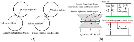
Figure 13.
Comprehensive schematic diagram of the structure and constitutive relationship for the bonded model: (a) schematic diagram of the bonded model; (b) schematic diagram of the constitutive relationship for the parallel bonded model.
The model’s characteristics are defined by five parameters: normal stiffness, tangential stiffness, normal strength, tangential strength, and bond radius. These parameters collectively define the linear elastic deformation, friction, and viscous behavior between particle elements. Adjusting these parameters allows for a more accurate simulation of the mechanical properties of rock materials, enhancing the accuracy and reliability of the simulations.
4. Results and Discussion
4.1. Physical Experiments and Numerical Simulations
The main materials used for the actual concrete specimens included cement, fine aggregates, coarse aggregates, water, and admixtures. The cement used was ordinary Portland cement. The fine aggregate was natural river sand, and the coarse aggregate was crushed stone (Figure 14a). Tap water was used. The admixture was PCA-I type high-efficiency water reducer. The concrete mix proportions were configured according to design requirements. The concrete strength grade used in the experiments was C30, with the specific mix proportions provided in Table 1. It should be noted that the concrete mix components in this study were not scaled down to match the characteristic dimensions. For all specimens, the maximum size of the coarse aggregate was approximately 30 mm. The mass contents of the cement and water were 340 kg/m3 and 178 kg/m3, respectively. The water-to-cement ratio was approximately 0.52. The total mass content of the concrete (Sum) was 2278 kg/m3. The prepared concrete mix was poured into standard cubic molds with dimensions of 150 mm × 150 mm × 150 mm. To ensure that the specimens were compact and uniform, tamping rods or vibrating tables were used to consolidate the concrete during pouring. After pouring, the surface was leveled with a scraper, and a damp cloth was placed over the specimens after initial setting to prevent water evaporation. After demolding, the specimens were immediately placed in a curing room under standard conditions with a temperature of 20 ± 2 °C and a relative humidity of no less than 95%. The curing duration was 28 days, during which the specimens were kept moist (Figure 14b). Compressive strength tests were performed on the concrete specimens using a hydraulic pressure testing machine (Figure 14c). The loading rate of the testing machine was 0.5 MPa/s, ensuring uniform and stable loading. The ultimate load values for the three specimens were 753.75 kN, 778.5 kN, and 747 kN, respectively (Figure 15). The average compressive strength was calculated to be 33.8 MPa.
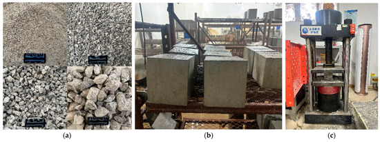
Figure 14.
Compressive strength test of standard concrete specimens: (a) Aggregates; (b) concrete specimens; (c) hydraulic testing machine.

Table 1.
Concrete mixture proportions utilized.
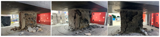
Figure 15.
Concrete specimen after uniaxial compressive strength test.
At the mesoscopic scale, concrete is typically considered a three-phase composite material consisting of aggregate particles, a mortar matrix, and an interfacial transition zone (ITZ) between the first two phases. Evaluating the composite behavior of concrete at the mesoscale requires generating a random aggregate structure in which the shape, size, and distribution of the aggregate particles statistically resemble those of real concrete. Additionally, aggregates, including fine and coarse aggregates, usually account for 60%–80% of concrete’s volume, significantly influencing its performance, mix proportions, and cost-efficiency. For simplicity in this study, fine aggregates and cement paste are combined into the mortar matrix. Coarse aggregates make up approximately 40%–50% of the concrete’s volume [47]. The shape of aggregate particles depends on the type of aggregate. Gravel aggregates are generally rounded, while crushed-stone aggregates are angular [34]. Modeling with spherical aggregates can satisfy the grading distribution in real concrete but lacks accuracy in representing aggregate morphology. Using ellipsoidal aggregates for modeling can meet three parameters of real concrete—grading, aspect ratio, and angular distribution—but still falls short of capturing the aggregate’s true morphology. Modeling with polygonal aggregates can satisfy four parameters: grading, aspect ratio, angular distribution, and roundness. Grading refers to determining the particle size distribution of aggregates, often expressed as a cumulative percentage passing through a series of sieve sizes. This can be represented through formulas, tables, or charts. In practice, one of the most well-known and widely accepted aggregate distributions is the one proposed by Fuller. The Fuller curve-based aggregate grading provides optimal aggregate packing, generating more fine aggregate particles to maximize concrete density and macroscopic strength. The grading curve formula is
where P is the cumulative percentage passing a sieve with aperture diameter D, and Dmax is the maximum size of aggregate particles.
In order to determine the mechanical parameters, especially the compressive strengths, a cubic concrete sample size of 150 mm × 150 mm × 150 mm was established, as presented in Figure 16. The concrete mix composition used in the numerical model was the same as that listed in Table 1. To ensure that the 3D three-phase random aggregate model accurately reflected the material composition and physical characteristics of the concrete used in the experiments, the mass-based mix proportions provided in Table 1 were systematically converted into volume fractions and mechanical input parameters required by the model. First, the volume fraction of coarse aggregates was derived by combining their mass proportion with the known densities of the constituent materials, and this value was used to define the aggregate content in the 3D model. Second, based on the actual composition of the concrete, the model was divided into three distinct phases: coarse aggregates, the mortar matrix, and the interfacial transition zone (ITZ). The shapes and sizes of the aggregates were randomly generated to match the maximum particle size and grading of the crushed stone used in the experiments. Finally, the mechanical properties of each phase—including Young’s modulus, Poisson’s ratio, and compressive strength—as well as the ITZ thickness, were determined based on the target strength grade of the experimental mix, the published literature, and known material characteristics. This parameterization ensures consistency between the numerical model and the experimental conditions in terms of both material composition and mechanical behavior, thereby providing a reliable basis for subsequent simulation analyses and result comparisons. The Fuller’s curve was utilized to describe the aggregate size distribution. The numbers of random aggregates within the particle size ranges of 5–10 mm and 10–30 mm are 1227 and 258, respectively. The major mechanical parameters of the three meso components used in the simulations are provided in Table 2. It is to be noted that Young’s modulus, Poisson’s ratio, the compressive strength of the aggregate particles, and the mortar matrix are obtained from the tests, while the mechanical properties of the ITZs are given with reasonable assumption [48]. The real typical thickness of the ITZ is about 0.05 mm; however, because of the limitation in computational capacity, it is impossible to use such small elements to model the real thickness of the ITZ.
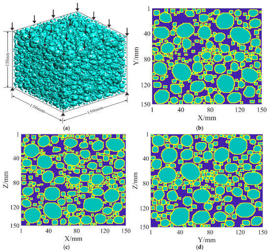
Figure 16.
Modeling of the proposed mesoscale numerical model: (a) uniaxial compressive simulation of concrete samples with dimensions of 150 mm × 150 mm × 150 mm, the arrows indicate the applied force on the top surface; (b) XY section of the concrete model; (c) XZ section of the concrete model; (d) YZ section of the concrete model. Green, yellow, and blue represent aggregate, ITZ, and mortar, respectively.
Table 2.
Mechanical parameters of the meso components.
In the concrete model generated, green, blue, and red spherical particles represent mortar, aggregate, and ITZ, respectively (Figure 17). It is worth noting that due to experimental limitations, it is challenging to measure the mechanical properties of the ITZ directly. In numerical simulations, the mechanical properties of the ITZ are typically described as weaker mechanical parameters of the mortar matrix, with the ITZ assumed to range between 30% and 80% of the mortar matrix’s strength [49,50].
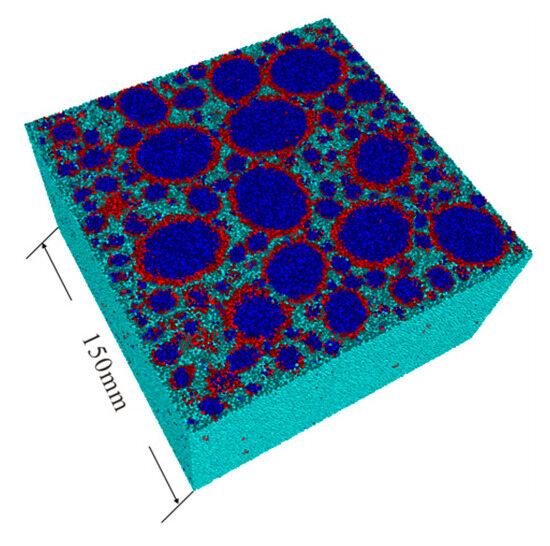
Figure 17.
DEM three-dimensional numerical model. Blue, red, and green represent aggregate, ITZ, and mortar, respectively.
In this study, concrete is treated as a three-phase composite material consisting of a mortar matrix, coarse aggregates, and an ITZ. The physical and mechanical properties of each phase are summarized in Table 2. The elastic modulus, Poisson’s ratio, and compressive strength of the mortar matrix and aggregates were obtained from standard specimen tests. Since the ITZ is difficult to isolate and test directly in experiments, its mechanical parameters were adopted from the existing literature [49,50], and its strength was set to approximately 75% of that of the mortar. Regarding boundary conditions, uniaxial compression was applied by imposing vertical displacement on the top and bottom loading plates. The bottom plate was fully fixed in all directions, while the top plate was allowed to move only in the vertical direction. The lateral sides of the specimen were left unconstrained, employing free boundary conditions to better replicate realistic loading conditions. To meet the requirements of quasi-static loading, a time-stepping algorithm was used for the simulation, with the total number of steps reaching several tens of thousands. During each time step, the forces and displacements between particles were updated. The simulation was terminated when the axial stress dropped to 80% of its peak value [51]. For model validation, the simulated specimen’s dimensions (150 mm × 150 mm × 150 mm), mix proportions (Table 1), maximum aggregate size (30 mm), and loading rate were all consistent with the experimental setup. The coarse aggregate used was natural crushed stone, with an elastic modulus set to 70 GPa, which is consistent with the properties of hard limestone rocks [48]. Figure 18a presents the simulation results under uniaxial compression with an ultimate strength of 31.1 MPa, corresponding to the experimental result of 33.8 MPa. The simulation results show good consistency with the experimental results. In this study, the mechanical parameters listed in Table 2 were adopted in the subsequent simulations. Figure 18b shows the numerical failure mode. Under uniaxial compression loading, the interfacial transition zone (ITZ) is the weakest phase in concrete, where numerous microcracks develop. Microcracks extending into the mortar form interfacial cracks, which eventually connect to form macroscopic cracks; this progression represents a typical feature of brittle failure in concrete. The simulated failure mode is consistent with the results observed in laboratory experiments. Furthermore, the results of this study were compared with those obtained from an existing two-dimensional (2D) mesoscale finite element model [52]. Although the 2D model also incorporated randomly distributed coarse aggregates to evaluate the mechanical behavior of concrete, and its resulting stress–strain curve (Figure 18a) exhibits a similar macroscopic trend to our numerical results, it is inherently limited to in-plane mechanical behavior and thus fails to accurately capture the three-dimensional characteristics of crack propagation. In contrast, the 3D mesoscale model developed in this study not only accurately reproduces the stochastic distribution of aggregate sizes but also fully captures the spatial distribution of cracks within the specimen volume. The predicted strain localization zones and crack paths show good agreement with experimentally observed fracture morphologies. In the 2D model, cracks tend to concentrate along the weakest plane, and their inclination and continuity are restricted by the simplified treatment of the thickness direction, making it difficult to reflect the complex through-thickness failure modes. Overall, although 2D simulations offer certain advantages in computational efficiency and in capturing general mechanical trends, the 3D mesoscale model provides more realistic and detailed representations of crack evolution paths, spatial failure mechanisms, and size effects. This makes it a more reliable numerical tool for investigating concrete fracture mechanisms and for applications at the engineering scale.
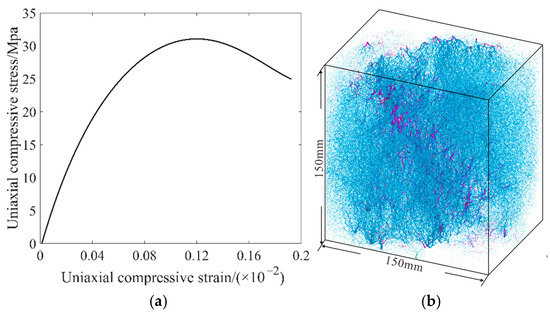
Figure 18.
Concrete uniaxial compression stress–strain curve and failure mode: (a) uniaxial compressive stress–strain curve; (b) uniaxial compressive failure mode, the purple area represents the damaged region, and the blue area indicates the undamaged region.
4.2. The Influence of Aggregate Shape Content on the Compressive Strength of Concrete Specimens
Commonly used aggregates in concrete include pebbles, crushed stone, and gravel. Pebbles are natural aggregates that are round or nearly round in shape, typically obtained from natural deposits such as rivers, lakes, or beaches. Their surfaces are generally smooth, and their rounded shape contributes to better workability (flowability and ease of handling) of concrete. Crushed stone is an aggregate produced by mechanically crushing natural rocks. It is usually irregular and angular in shape, with rough surfaces. This type of aggregate bonds well with cement paste, enhancing the strength of the concrete. Gravel generally refers to irregularly shaped rock fragments formed through natural weathering or water flow. Compared to pebbles, gravel has a more irregular shape but smoother surfaces, falling between pebbles and crushed stone in terms of characteristics. In this study, spheres or ellipsoids are used to model pebbles, while irregular polyhedra are used to model crushed stone and gravel.
The coarse aggregates used in the experimental program were natural crushed stone, primarily composed of limestone. These aggregates exhibit irregular polyhedral shapes with pronounced angularity and complex geometrical features (Figure 14a). Therefore, it is necessary to investigate the influence of aggregate shape on the simulated compressive strength of concrete. To examine the effect of different aggregate geometries on the macroscopic mechanical behavior of concrete, three types of aggregate models were constructed in numerical simulations: spherical, ellipsoidal, and irregular polyhedral shapes. Among them, the irregular polyhedral aggregates were generated using a stochastic algorithm designed to closely approximate the geometrical characteristics of real crushed stone. The results indicate that aggregate shape has a noticeable influence on the simulated uniaxial compressive strength.
The 3D aggregate random generation method proposed in this study was used to create three models. Each model had dimensions of 150 mm × 150 mm × 150 mm and an aggregate volume fraction of 40%. The aggregate shapes included spherical, ellipsoidal, and irregular polyhedral forms (Figure 19). Figure 20 shows DEM three-dimensional numerical models of aggregates with different shapes. Figure 21 presents the compressive stress–strain curves of models with different aggregate shapes. The figure shows that for an aggregate volume fraction of 40%, specimens with polyhedral aggregates have the lowest compressive strength, while those with spherical and ellipsoidal aggregates exhibit similar compressive strength. This conclusion aligns well with previous findings [53,54,55].
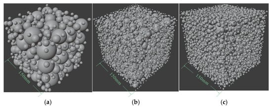
Figure 19.
Cubic samples containing differently shaped aggregates: (a) spherical aggregates; (b) ellipsoidal aggregates; (c) polyhedral aggregates.
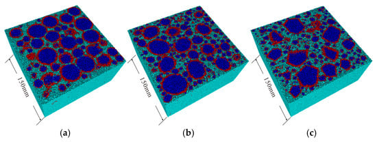
Figure 20.
DEM three-dimensional numerical models of aggregates with different shapes: (a) spherical aggregate model; (b) ellipsoidal aggregate model; (c) polyhedral aggregate model. Blue, red, and green represent aggregate, ITZ, and mortar, respectively.
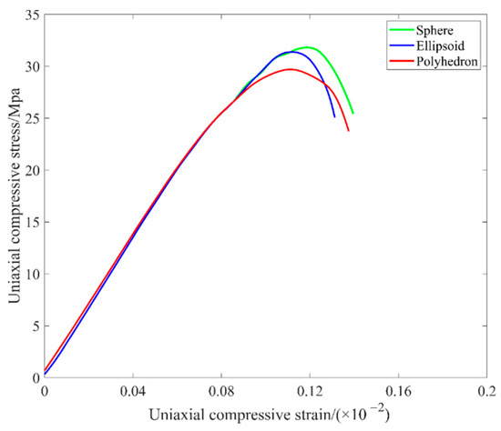
Figure 21.
Compressive stress–strain curves obtained from simulations of concrete with different aggregate shapes.
4.3. The Influence of Aggregate Particle Size on the Compressive Strength of Concrete Specimens
A two-graded concrete was selected, with model dimensions of 150 mm × 150 mm × 150 mm. The aggregate particle sizes were randomly distributed within the ranges of 5–10 mm and 10–30 mm, with a total aggregate content of 40%. Aggregates in the 5–10 mm range were uniformly distributed, while the 10–30 mm aggregates were divided into three groups based on the maximum particle size: Dmax = 20, 25, and 30 mm (Figure 22). This approach ensured that all other parameters remained constant, with only the maximum aggregate size varying. Figure 23 shows DEM three-dimensional numerical models with various maximum aggregate particle sizes. The stress–strain curves of specimens with different aggregate sizes are shown in Figure 24. It can be observed that the stress–strain curves in the elastic deformation region are quite similar. However, differences are evident in the peak stress and the softening stage, with some deviations near the yield point and peak stress. The compressive strength of the specimens decreases as the aggregate size increases, which is consistent with previous experimental results [52].
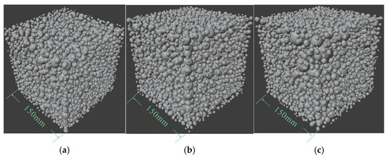
Figure 22.
Cubic samples containing various maximum aggregate particle sizes: (a) Dmax = 20 mm; (b) Dmax = 25 mm; (c) Dmax = 30 mm.
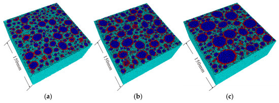
Figure 23.
DEM three-dimensional numerical models with various maximum aggregate particle sizes: (a) Dmax = 20 mm; (b) Dmax = 25 mm; (c) Dmax = 30 mm. Blue, red, and green represent aggregate, ITZ, and mortar, respectively.
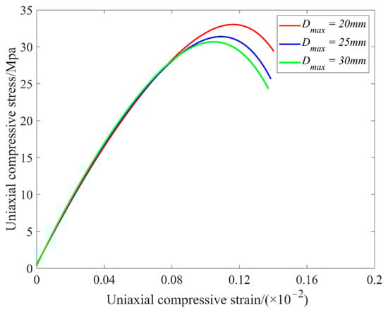
Figure 24.
Compressive stress–strain curves for cubes with different maximum aggregate particle sizes.
When the load is below 80% of the peak stress, the concrete material remains in the linear elastic damage phase. At this stage, the interfacial transition zone (ITZ) develops some relatively stable microcracks that have not yet interconnected or penetrated one another. Once the load exceeds 80% of the peak stress, irreversible plastic damage occurs within the concrete, and cracks begin to propagate unstably. Microcracks extend and connect to form larger cracks. The increase in aggregate size weakens the bonding performance of the ITZ, leading to a decline in compressive strength. In the initial elastic stage of the stress–strain curves, the curves corresponding to different maximum aggregate sizes nearly overlap, indicating that aggregate size has a negligible effect on the overall elastic stiffness of concrete. This is primarily because the deformation in this stage is dominated by the synergistic action between the mortar matrix and the aggregate skeleton, while the interfacial transition zone (ITZ) has not yet developed significant microcracks—only isolated and stable microcracks may appear, which do not cause substantial stress disturbances. However, once the material enters the inelastic stage, the peak stress decreases significantly with increasing maximum aggregate size. This phenomenon can be attributed to the fact that, under the same volume fraction, larger aggregates possess a smaller specific surface area, resulting in more concentrated stress at the mortar–aggregate interfaces. This exacerbates stress concentration in the ITZ and weakens its mechanical performance, promoting earlier initiation and faster coalescence of interfacial microcracks. In contrast, smaller aggregates can form a more uniform and compact particle structure, which helps to restrain crack propagation. As the aggregate size increases, size effects become more pronounced, leading to more severe local stress concentration and crack instability. Consequently, concrete with larger aggregates tends to enter the softening stage more abruptly after reaching the peak stress, and the failure process exhibits more brittle characteristics.
5. Conclusions
This study systematically investigates the mechanism by which aggregate shape and size affect the compressive performance of concrete by constructing a 3D three-phase mesoscale model and employing the discrete element method. The main conclusions are as follows:
- (1)
- To study the compressive performance of concrete, a three-dimensional three-phase mesoscale model composed of coarse aggregates, mortar, and the interfacial transition zone was constructed. The proposed aggregate generation method uses grid partitioning and conditional screening to achieve a random distribution of aggregates, avoiding aggregate overlap and significantly improving generation efficiency and accuracy. This model provides an effective tool for investigating the random distribution characteristics of aggregates in concrete.
- (2)
- The 3D random aggregate generation method introduced in this study has significant advantages: the computational time required to generate a single aggregate decreases rapidly as the number of already generated aggregates increases, effectively avoiding computational redundancy.
- (3)
- The discrete element method was used to simulate the effects of different aggregate shapes and maximum aggregate sizes on the compressive behavior of concrete. The simulation results reveal that increasing the maximum aggregate size from 20 mm to 30 mm leads to an 8% reduction in the peak compressive strength of concrete. Furthermore, under a constant aggregate volume fraction of 40%, the use of irregular polyhedral aggregates results in a decrease of approximately 7% in compressive strength compared to spherical and ellipsoidal aggregates. These findings indicate that larger aggregate sizes and more irregular shapes tend to exacerbate interfacial stress concentrations and promote unstable crack propagation, ultimately compromising the overall load-bearing capacity of concrete.
Additionally, this study considers only one type of coarse aggregate and assumes uniform properties for the interfacial transition zone (ITZ). The effects of aggregate type diversity and ITZ variability on crack development were not explored, limiting the model’s ability to simulate interface damage. Certainly, the model still has some limitations when applied to more complex concrete systems, such as fiber-reinforced concrete or multiphase coarse-grained concrete. At present, the model is not yet capable of accurately capturing interfacial behavior and the interactions between fibers and the matrix. Future research should incorporate multi-scale modeling strategies and improve constitutive relationships for different material phases. Future research should address these factors to improve model adaptability and engineering relevance.
Author Contributions
Conceptualization, S.W. and H.Z.; methodology, D.W. and X.W.; software, D.W.; validation, H.Z.; formal analysis, S.W.; investigation, S.W. and M.C.; resources, H.Z.; data curation, H.Z.; writing—original draft preparation, S.W. and H.Z.; writing—review and editing, S.W. and D.W.; visualization, H.Z.; supervision, S.W.; project administration, S.W.; funding acquisition, S.W. and X.W. All authors have read and agreed to the published version of the manuscript.
Funding
This research was funded by the National Key Research and Development Program of China, grant number 2023YFC2907600 and project ZR2022QD056 supported by Shandong Provincial Natural Science Foundation, and Qingdao Postdoctoral Science Foundation, grant number QDBSH20240101037.
Institutional Review Board Statement
Not applicable.
Informed Consent Statement
Not applicable.
Data Availability Statement
Data will be made available on request.
Conflicts of Interest
The authors declare no conflicts of interest.
References
- Ren, Q.; Pacheco, J.; de Brito, J. Methods for the modelling of concrete mesostructures: A critical review. Constr. Build. Mater. 2023, 408, 133570. [Google Scholar] [CrossRef]
- Xiong, Q.; Wang, X.; Jivkov, A.P. A 3D multi-phase meso-scale model for modelling coupling of damage and transport properties in concrete. Cem. Concr. Compos. 2020, 109, 103545. [Google Scholar] [CrossRef]
- Bai, F.; Li, Y.; Liu, L.; Li, X.; Liu, W. An efficient and high-volume fraction 3D mesoscale modeling framework for concrete and cementitious composite materials. Compos. Struct. 2023, 325, 117576. [Google Scholar] [CrossRef]
- Diehl, M.; Wang, D.; Liu, C.; Mianroodi, J.R.; Han, F.; Ma, D.; Kok, P.J.J.; Roters, F.; Shanthraj, P. Solving Material Mechanics and Multiphysics Problems of Metals with Complex Microstructures Using DAMASK—The Düsseldorf Advanced Material Simulation Kit. Adv. Eng. Mater. 2020, 22, 1901044. [Google Scholar] [CrossRef]
- Wang, D.; Shanthraj, P.; Springer, H.; Raabe, D. Particle-induced damage in Fe–TiB2 high stiffness metal matrix composite steels. Mater. Des. 2018, 160, 557–571. [Google Scholar] [CrossRef]
- Xiao, J.; Lv, Z.; Duan, Z.; Zhang, C. Pore structure characteristics, modulation and its effect on concrete properties: A review. Constr. Build. Mater. 2023, 397, 132430. [Google Scholar] [CrossRef]
- Xia, Y.; Wu, W.; Yang, Y.; Fu, X. Mesoscopic study of concrete with random aggregate model using phase field method. Constr. Build. Mater. 2021, 310, 125199. [Google Scholar] [CrossRef]
- Chen, T.; Xiao, S. Three-dimensional mesoscale modeling of concrete with convex aggregate based on motion simulation. Constr. Build. Mater. 2021, 277, 122257. [Google Scholar] [CrossRef]
- Li, H.; Huang, Y.; Yang, Z.; Yu, K.; Li, Q.M. 3D meso-scale fracture modelling of concrete with random aggregates using a phase-field regularized cohesive zone model. Int. J. Solids Struct. 2022, 256, 111960. [Google Scholar] [CrossRef]
- Wang, X.F.; Yang, Z.J.; Yates, J.R.; Jivkov, A.P.; Zhang, C. Monte Carlo simulations of mesoscale fracture modelling of concrete with random aggregates and pores. Constr. Build. Mater. 2015, 75, 35–45. [Google Scholar] [CrossRef]
- Zhang, S.; Hamed, E.; Song, C. An image-based meso-scale model for the hygro-mechanical time-dependent analysis of concrete. Comput. Mech. 2023, 72, 1191–1214. [Google Scholar] [CrossRef]
- Alwash, M.; Breysse, D.; Sbartaï, Z.M. Using Monte-Carlo simulations to evaluate the efficiency of different strategies for nondestructive assessment of concrete strength. Mater. Struct. 2017, 50, 90. [Google Scholar] [CrossRef]
- Gong, F.; Yang, L.; Wang, Z.; Jia, J.; Ning, Y.; Ueda, T. Mesoscale discrete analysis of mechanical properties of recycled aggregate concrete based on Voronoi mesh. Constr. Build. Mater. 2023, 370, 130649. [Google Scholar] [CrossRef]
- Wang, J.; Yu, X.; Fu, Y.; Zhou, G. A 3D Meso-Scale Model and Numerical Uniaxial Compression Tests on Concrete with the Consideration of the Friction Effect. Materials 2024, 17, 1204. [Google Scholar] [CrossRef] [PubMed]
- Zhou, R.; Song, Z.; Lu, Y. 3D mesoscale finite element modelling of concrete. Comput. Struct. 2017, 192, 96–113. [Google Scholar] [CrossRef]
- Ouyang, H.; Chen, X. 3D meso-scale modeling of concrete with a local background grid method. Constr. Build. Mater. 2020, 257, 119382. [Google Scholar] [CrossRef]
- Yang, X.; Wang, M. Fractal dimension analysis of aggregate packing process: A numerical case study on concrete simulation. Constr. Build. Mater. 2021, 270, 121376. [Google Scholar] [CrossRef]
- Xu, W.; Fu, J.; Hua, R.; Han, F. ITZ volume fraction and thermal conductivity of concrete: A unified random packing model for gravels and crushed rocks. J. Build. Eng. 2024, 90, 109457. [Google Scholar] [CrossRef]
- Wang, J.; Jivkov, A.P.; Engelberg, D.L.; Li, Q. Image-Based vs. Parametric Modelling of Concrete Meso-Structures. Materials 2022, 15, 704. [Google Scholar] [CrossRef]
- Song, Y.; Shen, C.; Damiani, R.M.; Lange, D.A. Image-based restoration of the concrete void system using 2D-to-3D unfolding technique. Constr. Build. Mater. 2021, 270, 121476. [Google Scholar] [CrossRef]
- Pan, G.; Song, T.; Li, P.; Jia, W.; Deng, Y. Review on finite element analysis of meso-structure model of concrete. J. Mater. Sci. 2025, 60, 32–62. [Google Scholar] [CrossRef]
- Xu, W.; Han, Z.; Tao, L.; Ding, Q.; Ma, H. Random non-convex particle model for the fraction of interfacial transition zones (ITZs) in fully-graded concrete. Powder Technol. 2018, 323, 301–309. [Google Scholar] [CrossRef]
- Paruthi, S.; Husain, A.; Alam, P.; Khan, A.H.; Hasan, M.A.; Magbool, H.M. A review on material mix proportion and strength influence parameters of geopolymer concrete: Application of ANN model for GPC strength prediction. Constr. Build. Mater. 2022, 356, 129253. [Google Scholar] [CrossRef]
- Ren, D.; Liu, X.; Cui, B.; Wang, E.; Ma, Q.; Yan, F.; Xie, W. Meso-crack evolution based constitutive model for concrete material under compression. Compos. Part B Eng. 2023, 265, 110956. [Google Scholar] [CrossRef]
- Zhou, R.; Lu, Y.; Wang, L.-G.; Chen, H.-M. Mesoscale modelling of size effect on the evolution of fracture process zone in concrete. Eng. Fract. Mech. 2021, 245, 107559. [Google Scholar] [CrossRef]
- Sun, Y.; Roubin, E.; Shao, J.; Colliat, J.-B. Meso-scale Finite Element modeling of the Fracture Process Zone evolution for concrete. Theor. Appl. Fract. Mech. 2023, 125, 103869. [Google Scholar] [CrossRef]
- Baktheer, A.; Martínez-Pañeda, E.; Aldakheel, F. Phase field cohesive zone modeling for fatigue crack propagation in quasi-brittle materials. Comput. Methods Appl. Mech. Eng. 2024, 422, 116834. [Google Scholar] [CrossRef]
- Schröder, J.; Pise, M.; Brands, D.; Gebuhr, G.; Anders, S. Phase-field modeling of fracture in high performance concrete during low-cycle fatigue: Numerical calibration and experimental validation. Comput. Methods Appl. Mech. Eng. 2022, 398, 115181. [Google Scholar] [CrossRef]
- Wu, Z.; Lei, J.; Ye, C.; Yu, C.; Zhao, J. Coupled FDM-DEM simulations of axial compression tests on FRP-confined concrete specimens. Constr. Build. Mater. 2022, 351, 128885. [Google Scholar] [CrossRef]
- Mansour, D.M.; Ebid, A.M. Predicting thermal behavior of mass concrete elements using 3D finite difference model. Asian J. Civ. Eng. 2024, 25, 1601–1611. [Google Scholar] [CrossRef]
- Nitka, M. Static and dynamic concrete calculations: Breakable aggregates in DEM model. J. Build. Eng. 2024, 89, 109006. [Google Scholar] [CrossRef]
- Nitka, M.; Tejchman, J. Modelling of concrete behaviour in uniaxial compression and tension with DEM. Granul. Matter 2015, 17, 145–164. [Google Scholar] [CrossRef]
- Wang, P.; Gao, N.; Ji, K.; Stewart, L.; Arson, C. DEM analysis on the role of aggregates on concrete strength. Comput. Geotech. 2020, 119, 103290. [Google Scholar] [CrossRef]
- Wang, Z.M.; Kwan, A.K.H.; Chan, H.C. Mesoscopic study of concrete I: Generation of random aggregate structure and finite element mesh. Comput. Struct. 1999, 70, 533–544. [Google Scholar] [CrossRef]
- Chen, J.; Wang, H.; Dan, H.; Xie, Y. Random Modeling of Three-Dimensional Heterogeneous Microstructure of Asphalt Concrete for Mechanical Analysis. J. Eng. Mech. 2018, 144, 04018083. [Google Scholar] [CrossRef]
- Ma, H.; Xu, W.; Li, Y. Random aggregate model for mesoscopic structures and mechanical analysis of fully-graded concrete. Comput. Struct. 2016, 177, 103–113. [Google Scholar] [CrossRef]
- Sun, Y.; Wei, X.; Gong, H.; Du, C.; Wang, W.; Chen, J. A two-dimensional random aggregate structure generation method: Determining effective thermo-mechanical properties of asphalt concrete. Mech. Mater. 2020, 148, 103510. [Google Scholar] [CrossRef]
- Ma, H.; Song, L.; Xu, W. A novel numerical scheme for random parameterized convex aggregate models with a high-volume fraction of aggregates in concrete-like granular materials. Comput. Struct. 2018, 209, 57–64. [Google Scholar] [CrossRef]
- Wei, S.; Shen, J.; Yang, W.; Li, Z.; Di, S.; Ma, C. Application of the renormalization group approach for permeability estimation in digital rocks. J. Pet. Sci. Eng. 2019, 179, 631–644. [Google Scholar] [CrossRef]
- Wei, S.; Wang, D.; Wang, X.; Zhang, H.; Cao, H.; Liu, Q. Research on the random generation model of 2D irregular aggregates in concrete based on fast grid region division method and its ground penetrating radar characteristics. Case Stud. Constr. Mater. 2024, 21, e03932. [Google Scholar] [CrossRef]
- Marples, C.R.; Williams, P.M. The Golden Ratio in Nature: A Tour across Length Scales. Symmetry 2022, 14, 2059. [Google Scholar] [CrossRef]
- Sen, S.K.; Agarwal, R.P. Golden ratio in science, as random sequence source, its computation and beyond. Comput. Math. Appl. 2008, 56, 469–498. [Google Scholar] [CrossRef]
- Zhang, J.; Ma, R.; Pan, Z.; Zhou, H. Review of Mesoscale Geometric Models of Concrete Materials. Buildings 2023, 13, 2428. [Google Scholar] [CrossRef]
- Wei, D.; Hurley, R.C.; Poh, L.H.; Dias-da-Costa, D.; Gan, Y. The role of particle morphology on concrete fracture behaviour: A meso-scale modelling approach. Cem. Concr. Res. 2020, 134, 106096. [Google Scholar] [CrossRef]
- Masad, E.; Olcott, D.; White, T.; Tashman, L. Correlation of Fine Aggregate Imaging Shape Indices with Asphalt Mixture Performance. Transp. Res. Rec. J. Transp. Res. Board 2001, 1757, 148–156. [Google Scholar] [CrossRef]
- Qiu, W.; Fu, S.; Ye, J. Auto-generation methodology of complex-shaped coarse aggregate set of 3D concrete numerical test specimen. Constr. Build. Mater. 2019, 217, 612–625. [Google Scholar] [CrossRef]
- Wriggers, P.; Moftah, S.O. Mesoscale models for concrete: Homogenisation and damage behaviour. Finite Elem. Anal. Des. 2006, 42, 623–636. [Google Scholar] [CrossRef]
- Jin, L.; Zhang, S.; Li, D.; Xu, H.; Du, X.; Li, Z. A combined experimental and numerical analysis on the seismic behavior of short reinforced concrete columns with different structural sizes and axial compression ratios. Int. J. Damage Mech. 2018, 27, 1416–1447. [Google Scholar] [CrossRef]
- Liao, K.-Y.; Chang, P.-K.; Peng, Y.-N.; Yang, C.-C. A study on characteristics of interfacial transition zone in concrete. Cem. Concr. Res. 2004, 34, 977–989. [Google Scholar] [CrossRef]
- Zhang, S.; Zhang, C.; Liao, L.; Wang, C. Numerical study of the effect of ITZ on the failure behaviour of concrete by using particle element modelling. Constr. Build. Mater. 2018, 170, 776–789. [Google Scholar] [CrossRef]
- Li, J.; Zhang, J.; Qian, G.; Zheng, J.; Zhang, Y. Three-Dimensional Simulation of Aggregate and Asphalt Mixture Using Parameterized Shape and Size Gradation. J. Mater. Civ. Eng. 2019, 31, 04019004. [Google Scholar] [CrossRef]
- Zheng, Y.; Zhang, Y.; Zhuo, J.; Zhang, P.; Hu, S. Mesoscale synergistic effect mechanism of aggregate grading and specimen size on compressive strength of concrete with large aggregate size. Constr. Build. Mater. 2023, 367, 130346. [Google Scholar] [CrossRef]
- Zhou, X.; Xie, Y.; Long, G.; Li, J. Effect of surface characteristics of aggregates on the compressive damage of high-strength concrete based on 3D discrete element method. Constr. Build. Mater. 2021, 301, 124101. [Google Scholar] [CrossRef]
- Ghosh, S.; Dhang, N.; Deb, A. Influence of aggregate geometry and material fabric on tensile cracking in concrete. Eng. Fract. Mech. 2020, 239, 107321. [Google Scholar] [CrossRef]
- Wang, X.; Zhang, M.; Jivkov, A.P. Computational technology for analysis of 3D meso-structure effects on damage and failure of concrete. Int. J. Solids Struct. 2016, 80, 310–333. [Google Scholar] [CrossRef]
Disclaimer/Publisher’s Note: The statements, opinions and data contained in all publications are solely those of the individual author(s) and contributor(s) and not of MDPI and/or the editor(s). MDPI and/or the editor(s) disclaim responsibility for any injury to people or property resulting from any ideas, methods, instructions or products referred to in the content. |
© 2025 by the authors. Licensee MDPI, Basel, Switzerland. This article is an open access article distributed under the terms and conditions of the Creative Commons Attribution (CC BY) license (https://creativecommons.org/licenses/by/4.0/).