Automated Assessment of Marine Steel Corrosion Using Visible–Near-Infrared Hyperspectral Imaging

Abstract

Marine steel structures face severe corrosion risks due to harsh environmental conditions, posing significant logistical, economic, and safety challenges for inspection and maintenance. Traditional corrosion assessment methods are costly, labor-intensive, and potentially hazardous. This study evaluated the capabilities of visible-to-near-infrared hyperspectral imaging (HSI) for automating corrosion detection and severity classification in steel samples subjected to accelerated corrosion conditions simulating marine exposure. Marine steel coupons were partially coated to simulate protective paint and immersed in natural brackish water from the Panama Canal, creating varying corrosion levels. Hyperspectral images were acquired in controlled illumination conditions, calibrated radiometrically, and reduced in dimensionality via principal component analysis (PCA). Four machine learning models, including k-nearest neighbors, support vector machine, random forest, and multilayer perceptron, were tested for classifying corrosion severity. The multilayer perceptron achieved the highest accuracy at 96.18%, clearly distinguishing among five defined corrosion stages. These findings demonstrate that hyperspectral imaging, coupled with machine learning techniques, provides a viable, accurate, non-destructive methodology for assessing marine steel corrosion, potentially reducing costs, improving safety, and streamlining maintenance procedures.

1. Introduction

Marine vessels and offshore structures operate in highly corrosive environments. The marine atmosphere combines humidity, salt spray, temperature fluctuations, and pollutants that aggressively attack steel surfaces through electrochemical processes [1,2]. Marine steel exposed in coastal and open-ocean conditions rapidly develops corrosion unless properly protected. For example, cyclic wetting by saltwater and high humidity in marine regions creates an electrolyte layer on steel that accelerates rust formation [3]. Over time, corrosion products can form in layers and alter the mechanical properties of the steel surface, sometimes offering partial protection [4] but often leading to further functional degradation [2]. As corrosion severity increases, the structural integrity of critical components (such as ship hull plates) is compromised; the effective cross-sectional area of load-bearing members is reduced, making them vulnerable to failure under operational loads [5]. Thus, regular inspection and maintenance of marine vessels are mandated to ensure safety and prevent structural failures.

Routine maintenance of ship hulls typically involves periodic dry-dock inspections (often at least twice every five years) where the vessel is removed from water and surfaces are cleaned, inspected, and recoated [2]. These scheduled inspections aim to detect corrosion damage and perform corrective actions before significant strength loss occurs. However, dry-docking is logistically complex and expensive. The cumulative costs of repeated dry-dock maintenance over a vessel’s life are substantial [6,7]. For instance, the cost of repairing and recoating a ship’s hull during a single dry-dock can range from approximately $ 0.2 million to $ 0.7 million [2]. In addition to direct costs, taking a vessel out of service for inspection incurs downtime losses. Furthermore, manual inspection of large structures is labor-intensive and often dangerous: inspectors must access vast steel surfaces (sometimes at heights or confined spaces), working long hours in the presence of hazardous substances such as lead-based paints, volatile and/or combustible solvents, or simply the marine environment itself. This exposes personnel to a high degree of risk and potential accidents. However, shipping regulations and standards require a human component in marine vessel inspection processes [8,9]. Thus, the development of methodologies to inspect for corrosion in a manner that can reduce extensive dry-docking operations or direct human involvement has the potential to introduce significant logistical, economic, and safety benefits.

Over the years, numerous non-destructive evaluation (NDE) techniques have been proposed to detect or monitor corrosion in steel structures. In laboratory settings, researchers have employed electrochemical methods such as electrical resistance methods [10], linear polarization resistance [11], and electrochemical impedance spectroscopy (EIS) [12] to quantitatively assess corrosion rates. Other approaches include electromagnetic techniques such as eddy current testing, which can detect flaws or thinning under coatings [13], and various forms of spectroscopy to identify corrosion products. For example, Raman spectroscopy [14,15,16] and Fourier-transform infrared (FTIR) spectroscopy can characterize iron oxide compounds formed on steel [17,18,19,20,21,22,23], while X-ray diffraction (XRD) [18,24,25,26,27] and X-ray photoelectron spectroscopy (XPS) provide crystallographic and surface chemical information about rust layers [19,28,29]. Scanning electron microscopy (SEM) is also used to examine corroded surfaces at high resolution [26], and thermographic methodologies can be used to evaluate spatial inconsistencies in hull thermal images [30]. These laboratory methods offer detailed insights but typically require extracted samples or contact probes, making them impractical for rapid inspection over large structures in the field.

Recently, attention has turned to developing in-situ and automated corrosion inspection techniques that can be deployed directly on structures. Vision-based methods, in particular, have shown promise for remote sensing of corrosion. High-resolution RGB cameras combined with digital image processing allow inspectors or algorithms to survey large surface areas quickly. By employing machine-learning-based techniques, features such as color changes, texture, and shape of corrosion spots can be automatically detected for further analysis. Early studies focused on color space transformations (e.g., converting RGB images to L*a*b* or HSI color spaces) to enhance rust visibility [31]. Texture analysis techniques, such as gray level co-occurrence matrix features, have also been applied to quantify the surface roughness associated with rust [31]. With the rise of deep learning, convolutional neural networks (CNNs) have been trained to recognize corrosion directly from photographs of steel structures. For instance, Yao et al. developed a CNN model to identify corrosion damage on ship hull plates from images [32]. Xu et al. used an ensemble of CNNs to classify the rust grade and rust coverage on steel surfaces [33]. More recently, Wang et al. presented an image recognition method to evaluate marine corrosion on Q420 steel, demonstrating high accuracy using deep learning on visible images [34]. Moreover, vision transformers are emerging as a viable tool for image analysis in a variety of detection and assessment tasks [35,36,37]. In this context, Vasan et al. developed a methodology for the detection of surface defects in images of steel using vision transformers [38]. These vision-based approaches can be deployed using drones or camera-equipped robots, enabling faster coverage of the large surfaces in marine vessel hulls. Their limitation, however, is that conventional color images provide limited spectral information in the form of three broad wavelength bands corresponding to red, green, and blue colors as perceived by the human eye. Subtle differences in corrosion chemistry or early-stage oxidation might not produce significant color differences, especially under varying lighting conditions. This can lead to false negatives/positives if a rust patch is camouflaged, unevenly shaded in the operational context of image capture, or if benign stains are misidentified as corrosion.

Parallel to these developments, robotic systems have been introduced to automate physical inspection tasks. For example, magnetic climbing robots can carry ultrasonic thickness gauges to measure steel plate thickness and detect metal loss due to corrosion [39]. Enjikalayil et al. demonstrated a robot that traverses a ship hull and performs autonomous ultrasonic thickness measurements, mapping corrosion-related thinning without human intervention. Other robotic developments focus on maintenance tasks such as the cleaning and recoating of marine vessel hulls. For instance, Le et al. (2021) developed a reconfigurable robotic system for hydro-blasting and cleaning corroded hull surfaces [40]. While robotic platforms can reduce human risk and access hard-to-reach areas, they typically still rely on traditional sensors (cameras, ultrasonic probes, etc.) for detection. The effectiveness of these systems is therefore tied to the capabilities and limitations of their individual sensing devices and their modalities.

Hyperspectral Imaging as an Alternative Sensing Modality

One emerging technology that offers enhanced detection capability is hyperspectral imaging (HSI). Hyperspectral imaging combines aspects of spectroscopy and imaging, capturing a detailed spectrum at each pixel of a 2D scene [17,41,42]. For these reasons, HSI acquisition devices are alternatively referred to as imaging spectrometers [43,44].

Whereas conventional imaging records only three broad channels corresponding to perceived red, green, and blue channels, HSI preserves the complete spectral profile returned from a scene, typically sampling dozens to hundreds of contiguous bands that cover the visible and near-infrared ranges [45]. Thus, the fine spectral granularity contained in a hyperspectral images enables accurate material recognition by analyzing each substance’s distinctive spectral fingerprint. Due to the fact that an individual material’s chemical composition dictates which wavelengths it preferentially absorbs or reflects, hyperspectral analysis can both discriminate among different materials and reveal impurities or subtle compositional variations within ostensibly similar samples [46,47]. HSI has been successfully applied in fields such as agriculture [48], environmental monitoring [49], food quality control [50,51], and art conservation [52,53] to identify materials or detect subtle changes invisible to the naked eye. Its high spectral resolution makes it a promising tool for corrosion detection, where the spectral characteristics of iron oxides (goethite, lepidocrocite, hematite, etc.) might be differentiated from bare metal or paint [42,54].

Several recent studies have demonstrated the potential of HSI for steel corrosion assessment. DeKerf et al. used shortwave-infrared HSI (up to 1700 nm) to identify four common corrosion minerals on steel (goethite, magnetite, lepidocrocite, and hematite) by comparing hyperspectral signatures to a reference spectral library [54]. Lavadiya et al. showed that HSI in the visible/NIR range can eliminate some of the ambiguity of visual inspection, successfully distinguishing corrosion caused by different chemical agents (acidic, saline, etc.) by using principal component analysis (PCA) on the spectra followed by an SVM classifier [42]. Yang et al. developed a non-contact method for grading the corrosion on transmission tower steel using HSI, comparing the performance of SVM and partial least squares discriminant analysis (PLS-DA) after spectral feature reduction; they found that both models could detect corrosion grades with good accuracy, with HSI providing a viable means to inspecting tower members that are otherwise difficult to access [41]. These studies demonstrate that HSI products contain the base information necessary for both the successful detection of corrosion and further inference of various aspects of its nature, such as corrosion severity or causes. In addition, they establish the capability of machine learning methodologies to extract and process the necessary information to deliver these insights accurately. HSI for corrosion inspection is still a nascent area, and optimal analysis techniques remain an open question [31]. In particular, the choice of machine learning model and the handling of high-dimensional spectral data are important considerations in the development of an HSI-based corrosion detection system.

The current article presents an experimental study evaluating hyperspectral imaging for corrosion detection and classification in steel coupons subjected to marine-like accelerated corrosion conditions. Marine-grade steel samples with controlled paint coverage were exposed to natural brackish water from the Panama Canal to simulate realistic marine corrosion at multiple severity levels. Hyperspectral images in the visible-to-near-infrared range were acquired under controlled illumination and preprocessed through radiometric calibration and dimensionality reduction using principal component analysis (PCA). Machine learning techniques, including k-nearest neighbors (k-NN), support vector machine (SVM), random forest (RF), and a multilayer perceptron (MLP) neural network, were then trained and compared in their capability to classify corrosion severity based on hyperspectral measurements. The results obtained confirm the capability of hyperspectral imaging coupled with machine learning methodologies to accurately differentiate corrosion states.

The rest of this article is organized as follows. Section 2 reviews current remote sensing methodologies for marine vessel inspection, including conventional visual imaging techniques, ultrasonic and electromagnetic non-destructive evaluation (NDE) methods, infrared thermography, and recent hyperspectral imaging approaches. Section 3 describes the materials and methods of our study, including the sample preparation, hyperspectral data acquisition, preprocessing steps, and the machine learning models and evaluation metrics employed. Section 4 presents the experimental results of the corrosion classification, comparing the performance of the different models and discussing the implications, advantages, and trade-offs of each. Finally, Section 5 concludes the paper by affirming the viability of HSI for marine corrosion inspection and suggesting directions for future work, such as extending the approach to real-world conditions and integrating chemical identification and standards-based classification.

2. Remote Sensing Methodologies for Marine Vessel Inspection

Hyperspectral imaging (HSI) presents a modern, data-driven approach that can augment corrosion inspections by providing rich spectral information for each point on a surface. As presented in Section 1, HSI captures images in a large number of spectral bands, effectively performing a statistically independent reflectance spectroscopy measurement at each pixel in the scene [55]. For corrosion detection, the premise is that different materials, such as intact paint, bare steel, and steel at various corrosion stages, have discriminable spectral signatures that can be discerned with high spectral resolution. In a context where an RGB image might show all corrosion as a similar brown color, an HSI system could potentially differentiate between, for instance, a light hydrated iron oxide and a darker magnetite-rich rust with previous knowledge of their individual spectral curves.

One advantage of HSI for this application is its ability to cover a spatial area, much like a conventional camera, while still being able to observe detailed chemical information. Thus, it can produce corrosion “maps” indicating not just the spatial distribution of present corrosion but also potentially what specific corrosion grade or product has formed. Zabalza et al. demonstrated that common iron oxide corrosion products (goethite, akaganeite, lepidocrocite, etc.) each have unique reflectance features in the visible-to-near-infrared range, enabling their identification via hyperspectral analysis [31]. In their work, samples of steel with various known rust minerals were distinguishable in VNIR HSI data. Similarly, Chen et al. used machine learning on hyperspectral data to classify corrosion on steel into three categories, reporting that including bands beyond the visible improved the classification robustness [56]. Additionally, Lavadiya et al. used HSI to differentiate the cause of corrosion, which is a considerably difficult approach to develop exclusively using RGB images. They prepared steel samples corroded under different chemical exposures, simulating common environmental factors leading to corrosion in steel surfaces, such as acid rain and salt spray. These differing factors produced surface corrosion of slightly different chemical composition. By applying PCA to reduce the hyperspectral data and training a support vector machine (SVM) model, their approach was able to accurately identify which corrosive agent was responsible for a given measured surface corrosion spectrum [42]. This inference modality and these capabilities are beyond the scope of conventional RGB imaging and highlight HSI’s utility for detailed material analysis in the field. Similarly, the work by DeKerf et al. demonstrated the possibility of quantitatively identifying specific minerals in the rust layer [54]. By using shortwave infrared (SWIR) hyperspectral imaging up to 2.5 µm and a reference spectral library of pure corrosion minerals, they employed a normalized spectral correlation algorithm to match image pixels to probable compounds. Their methodology was able to produce distributed abundance maps of different corrosion chemical compounds, which visually show the predomination of different compounds across the image. Such information is valuable because the type of oxide can indicate the corrosion mechanism and the protective quality of the rust layer in a specific context.

Other studies such as Yang et al. focus on corrosion grading or determining how advanced corrosion is. Using HSI data from steel samples corroded for varying durations (48 h up to 384 h), their study compared k-NN and PLS-DA models to perform automated corrosion grade classification [41]. They reported that both models achieved good accuracy, with performance depending on the feature extraction method (PCA vs. a specialized wavelength selection algorithm). It is worth highlighting that even the k-NN, a relatively computationally simple model, performed well when provided with meaningful spectral features, indicating that the spectral differences between early and late corrosion, while subtle, are learnable.

These works highlight that HSI-based approaches foster the development of models based on enriched datasets for corrosion detection, but they also indicate common challenges: HSI-based methods suffer from the well-studied Hughes’ phenomenon (also known as the curse of dimensionality), where the classification performance of these classification algorithms diminishes proportionally to increased spectral information [57,58,59]. In order to mitigate this, these methods require an additional dimensionality reduction step prior to their algorithmic classification. In addition, hyperspectral cameras can be prohibitively expensive, limiting their deployability across a variety of fields [60,61]. Further, HSI acquisition has additional considerations for ensuring data integrity, requiring either controlled or carefully measured lighting conditions and calibration procedures to produce reliable spectra [62,63]. Finally, the volume of data contained in an HSI is considerably larger than that of an RGB image, which raises computational and data transmission concerns for real-time use [58,61]. Regardless, the trend in the literature is that HSI is emerging as a promising addition to the inspector’s toolbox, especially as sensor technology improves, analysis algorithms become more efficient, and sensors costs are reduced due to miniaturization and economies of scale [64,65].

In the context of marine vessel inspection, hyperspectral imagers could be deployed via handheld devices, on static infrastructure dedicated to ship inspection, or mounted on drones/robots to remotely scan and evaluate large portions of a ship’s hull. Such an approach could aid in early corrosion detection even before it becomes visible or severe and classify the severity or type of corrosion for targeted maintenance. However, it is important to note that governing regulations regarding marine vessel inspection still oblige a flag-state-approved surveyor to carry out the statutory annual, intermediate, and five-year renewal surveys prescribed by SOLAS Chapter I (Regulations 7 and 10) [8] and the Harmonized System of Survey and Certification (HSSC) (A.1120(30) and A.1140(31)) [9]. Specifically, these requirements include at least one dry-dock bottom examination in every five-year cycle. Although the International Association of Classification Societies has, through Recommendation 42 (Rev 2, 2016), formally recognized “remote inspection techniques” such as drone-borne or hyperspectral imaging as equivalent means, these may only be used under the surveyor’s direct supervision and do not eliminate the need for conventional spot hammering, visual confirmation, or ultrasonic gauging where the surveyor deems it necessary [66]. In other words, any methodologies based on hyperspectral imaging for remote inspection and evaluation of marine vessel hulls would represent a powerful and convenient supplemental evaluation, with the potential to reduce time and cost requirements by allowing inspectors to focus on identified problem areas, but not be a replacement for the statutorily mandated evaluation procedures.

In the remainder of this paper, we focus on the application of our HSI approach to the classification of corrosion severity, and we compare different data processing and machine learning strategies in their ability to effectively handle the spectral data.

3. Materials and Methods

3.1. Sample Preparation and Accelerated Corrosion Exposure

In order to obtain representative data for corrosion at various levels of progression, steel coupons were prepared and subjected to controlled corrosive exposure for different durations.

Specifically, eight coupons of SAE 316 stainless steel measuring $4\times 4$ inches (approximately $10\times 10$ cm) were used. Each steel plate was polished to a clean metal surface finish at the start of the experiment. The plates were then partially coated with a protective paint to simulate a common ship maintenance scenario where some areas are painted and others are bare or have failing coating. In particular, six of the plates had about 50% of their surface area coated with a commercial matte anti-corrosion paint (leaving the rest of the steel exposed), while the remaining two plates were left unpainted (fully exposed). This arrangement created samples that had side-by-side regions of bare steel, which was vulnerable to corrosion, and protected steel with an industry-standard anti-corrosion coating. The intention was to use the painted portions as a “no corrosion” class in the dataset, and the unpainted portions, following their exposure to a corrosive environment, as corroded classes. For the purposes of training, the measurements from four steel coupons were used (one for each corrosion medium exposure step), while the images from the remaining coupons were used for validation.

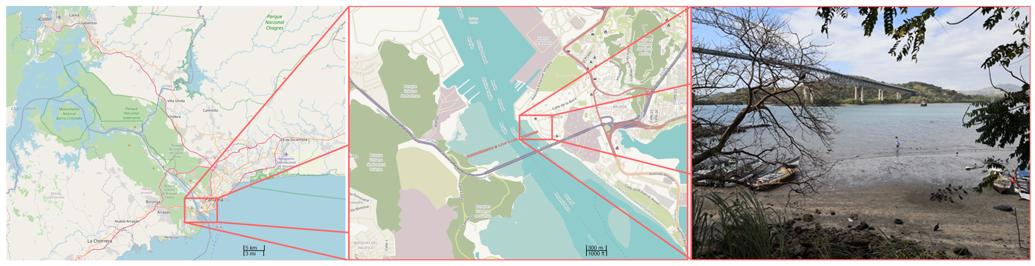
The steel coupons were subjected to accelerated corrosion via immersion in a brackish water solution over different time periods. Each plate was placed in a separate container filled with water obtained from the Panama Canal (Balboa area, Pacific entrance in Panama City). The Panama Canal water is a mix of sea and fresh water, containing salts and minerals that promote corrosion in steel, which is a reasonable proxy for marine coastal conditions. The extracted water sample was measured using a multiparametric water quality meter (HQ40d, Hach Lange GmbH, Dusseldorf, Germany), showing moderately saline conditions with a salinity 0.54 PSU, a slightly alkaline pH of 7.8, and dissolved oxygen levels of approximately 6.0 mg/L, influenced by frequent maritime traffic, consistent with previous observations [67]. For reference, the specific location where the corrosion medium was extracted is shown in Figure 1. The containers were kept at ambient laboratory temperature, between 25 and 30 °C, in order to mimic natural environmental conditions. No additional corrosive chemicals were added to the aqueous medium, and the natural salt content and oxygen availability in the water were relied upon to induce the corrosion process. The exposure durations for each coupon were 5 days, 10 days, 15 days, and 20 days, respectively. During these periods, the steel coupons were fully submerged and then taken out and sampled at the end of the allotted time.

Following their exposure to the corrosive medium, each steel coupon exhibited an incremental degree of corrosion on its unpainted regions proportional to its exposure time. The plate exposed for 5 days developed a light layer of yellowish-brown rust, with some metal still visible in places. The 10-day plate showed more extensive rust coverage and the 15-day plate further so, and the 20-day plate was almost entirely covered in a thick dark rust. The painted halves of the first three plates remained mostly uncorroded (the paint was intact, with only minor undercutting or edge corrosion, if any). These conditions provided a range of corrosion “levels”, which we associated with the exposure time: longer immersion produced more advanced corrosion. In our subsequent analysis, we defined five classes of interest:

• No corrosion (class C0): painted/protected steel with no visible corrosion.
• Light corrosion (class C1): corrosion after 5 days’ exposure (minimal surface rust).
• Moderate corrosion (class C2): corrosion after 10 days’ exposure.
• High corrosion (class C3): corrosion after 15 days’ exposure.
• Severe corrosion (class C4): corrosion after 20 days’ exposure (heaviest rust).

These categories align with increasing severity of rusting. Visually, C1 appeared as a thin rust film, C2 and C3 as progressively thicker and more uniformly distributed rust, and C4 as a dense dark rust covering the entire surface.

3.2. Hyperspectral Image Acquisition

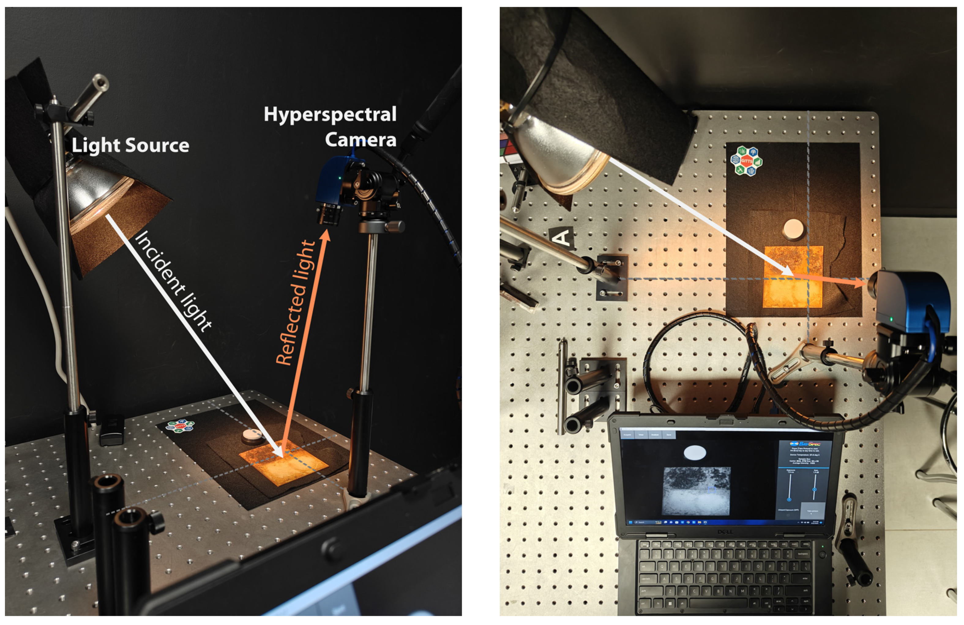
Following the corrosion exposure, the steel coupons were imaged using a hyperspectral camera in a controlled setup. The sampling procedure was performed using a GoldenEye snapshot hyperspectral camera (BaySpec, Inc., San Jose, CA, USA). The employed device captures images in 141 spectral bands from the visible-through-near-infrared range, specifically in the wavelengths from 400 nm to 1100 nm. The spectral resolution is such that contiguous bands are 5 nm apart. The imager features a CMOS detector with a spatial resolution of $648\times 488$ pixels. In other words, each hyperspectral image produced is structured as a $648\times 488\times 141$ data cube (x pixels by y pixels by 141 bands).

In order to ensure consistent illumination and reduce measurement noise across all samples, each steel coupon was imaged in a darkroom environment. In this environment, the samples were illuminated exclusively with a Halogen broadband light source at an angle perpendicular to the direction of the hyperspectral camera in order to reduce specular reflections [68]. Before capturing the sample images, we performed a calibration procedure using reference panels: a dark current frame (with the lens covered) and a Spectralon White Diffuse Reflectance Standard (LabSphere Inc., North Sutton, NH, USA) under the same lighting. The hyperspectral camera was mounted on a rigid structure on an optical table and focused in such a manner that the entire $4\times 4$ inch plate fit within the field of view. In order to reduce background noise and endure adequate contrast for HSI annotation, the sample was placed on light-absorbing material to ensure a homogeneous background. For illustrative purposes, an annotated image of the HSI acquisition configuration is presented in Figure 2. In order to further compensate for any possible spectral distribution drifts in the halogen lamp due to temperature variations [69], the diffuse reflectance standard was included in the hyperspectral measurements of all steel coupons.

The experimental specifications were as follows:

• Sensor: CMOS snapshot imaging spectrometer (BaySpec GoldenEye).
• Spatial resolution: $648\times 488$ pixels.
• Spectral range: 400–1100 nm (VIS + NIR).
• Number of bands: 141 (continuous).
• Interface: USB 3.0 (direct data acquisition to computer).
• Illumination: Tungsten–Halogen broadband light source with darkroom conditions.

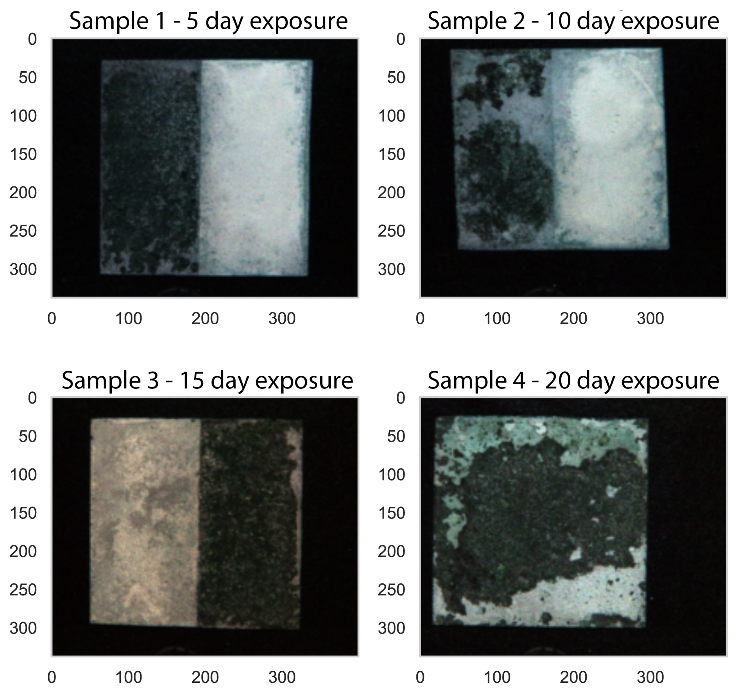
Following these preparations, a hyperspectral image was captured for each of the steel coupons. The resulting images showed the corroded and non-corroded regions clearly. For illustrative purposes, Figure 3 displays an RGB composite of the hyperspectral images for the four samples (using three selected bands mapped to R, G, B for visualization). In these RGB composites, the painted (unrusted) areas appear as the gray paint color, while the corroded areas appear in brownish tones, with darker brown for the more heavily corroded samples. Qualitatively, it could be observed in these images that that corrosion extent positively correlates with exposure time, for example in the difference between Sample 1 and Sample 4 in Figure 3. However, subtle differences between, for example, the 10-day and 15-day rust are not very distinguishable by the eye in the RGB view, which motivates the current work.

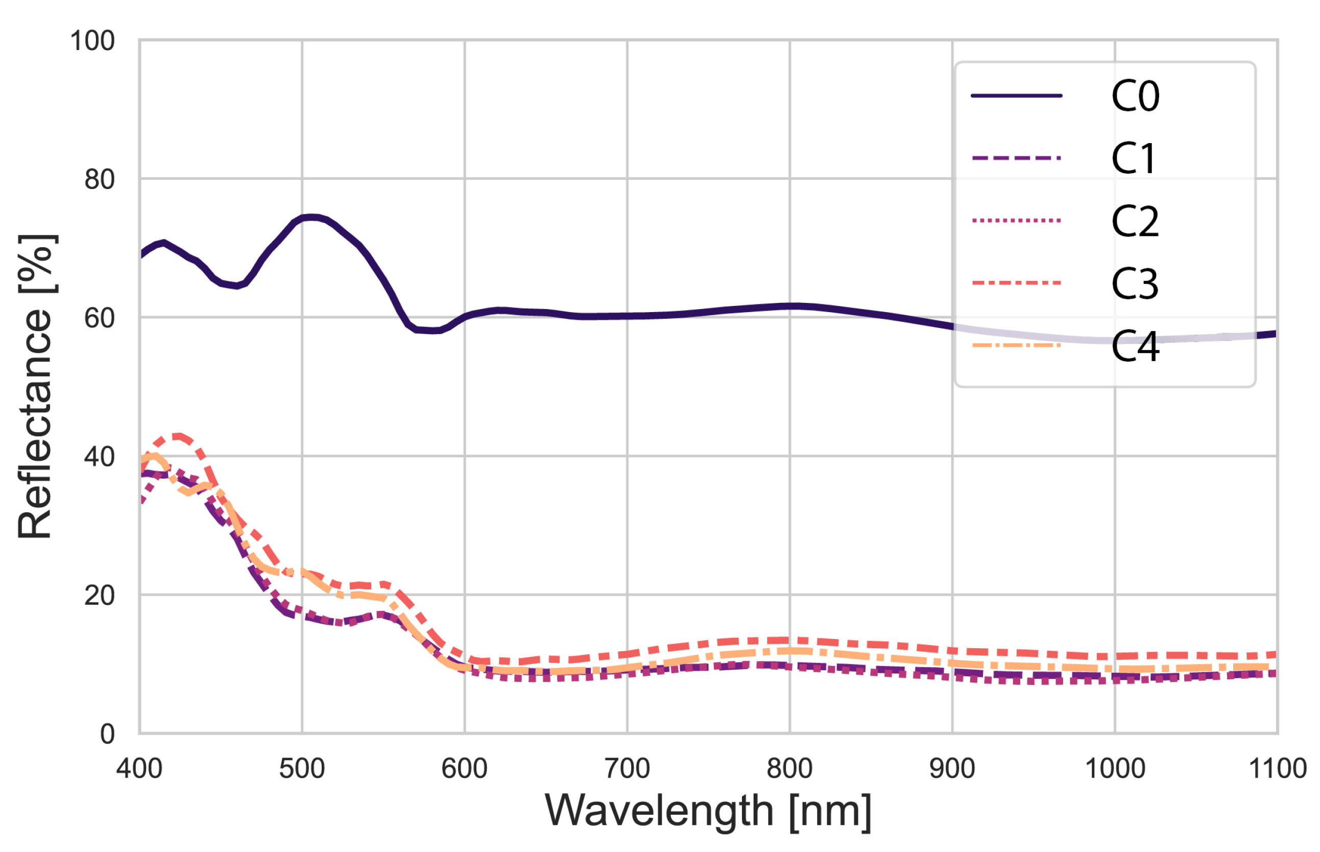
Following the capture of raw hyperspectral images, an intensity calibration procedure was performed in order to convert the raw sensor data to normalized reflectance values, as described in Section 3.3. Furthermore, from each calibrated hyperspectral image, summary spectral profiles for each corrosion exposure level were extracted. Figure 4 shows the mean spectral reflectance curves for each corrosion level (averaged over representative regions of each class). The spectral curve for the C0 class (no corrosion, painted) describes a uniform spectral behavior with high reflectance in the visible range, which is consistent with the corrosion-inhibiting white paint, whereas the corroded levels (1 through 4) have distinct spectral shapes, generally with lower reflectance in the blue and higher in the red/NIR, consistent with the reddish coloration of rust.

It is important to highlight the limitations of conventional RGB imaging compared to hyperspectral imaging for corrosion analysis. Typically, RGB imaging corresponds to broad spectral bands around approximately 640 nm (red), 550 nm (green), and 470 nm (blue). As evident from Figure 4, the measured reflectance values at these wavelengths do not provide sufficient statistical separability between closely related corrosion severity classes, being effective only at distinguishing a clear presence or absence of surface corrosion. This limitation further reinforces the advantage of hyperspectral imaging for corrosion severity classification.

3.3. Preprocessing of Hyperspectral Data

Raw hyperspectral images often contain systematic noise and artifacts due to the sensor and lighting. A critical preprocessing step is calibration using reference measurements. We performed dark current subtraction and white reference normalization on each image to obtain calibrated reflectance $R\left(\lambda \right)$ for each pixel. The calibration procedure is given by Equation (1).

$$R(x,y,\lambda )={\displaystyle \frac{I(x,y,\lambda )-I{(x,y,\lambda )}_{\mathrm{dark}}}{I{(x,y,\lambda )}_{\mathrm{white}}-I{(x,y,\lambda )}_{\mathrm{dark}}}},$$

(1)

where $I(x,y,\lambda )$ is the raw reflectance image measured by the camera for a given pixel at the spatial coordinates $(x,y)$ and wavelength $\lambda$; $I{(x,y,\lambda )}_{\mathrm{dark}}$ is the intensity recorded in a dark frame with the camera lens covered, representing sensor offset and dark noise; and $I{(x,y,\lambda )}_{\mathrm{white}}$ is the intensity recorded from the white reference standard under the same lighting, which directly represents the illumination spectrum and is assumed to be a 100% reflectance baseline. In an ideal scenario, applying Equation (1) yields the fraction of light reflected by the sample at each wavelength, where the values of $R(x,y,\lambda )\in (0,1)$.

In practice, we found that the dark current images for the hyperspectral camera utilized were uniformly very close or equal to zero relative to the target image intensities throughout the sampling operations due to stable environmental temperatures. Due to this, calibration was performed exclusively using the white reflectance reference for simplicity. Thus, Equation (1) was reformulated as presented in Equation (2)

$$R(x,y,\lambda )\approx {\displaystyle \frac{I(x,y,\lambda )}{I{(x,y,\lambda )}_{\mathrm{white}}}},$$

(2)

given the negligible contents of $I{(x,y,\lambda )}_{\mathrm{dark}}$. This simplification did not noticeably affect the results, and it streamlined the capture process by not requiring dark frames for every acquisition under laboratory conditions and temperature dynamics. Following the calibration procedure, each hyperspectral image’s pixel values represented normalized reflectance, ensuring consistent measurements across all samples for machine learning model training.

Following the intensity normalization step, the high dimensionality and correlation of hyperspectral data were addressed. Each pixel’s spectrum contains its normalized intensity across 141 bands, many of which are highly correlated, particularly in adjacent wavelengths, despite being statistically independent measurements. The presence of any measurement noise in individual bands, coupled with the redundancy in information, can pose challenges for certain machine learning models, both in terms of computational cost and risk of overfitting [57]. A common technique to overcome this is principal component analysis (PCA) [70,71].

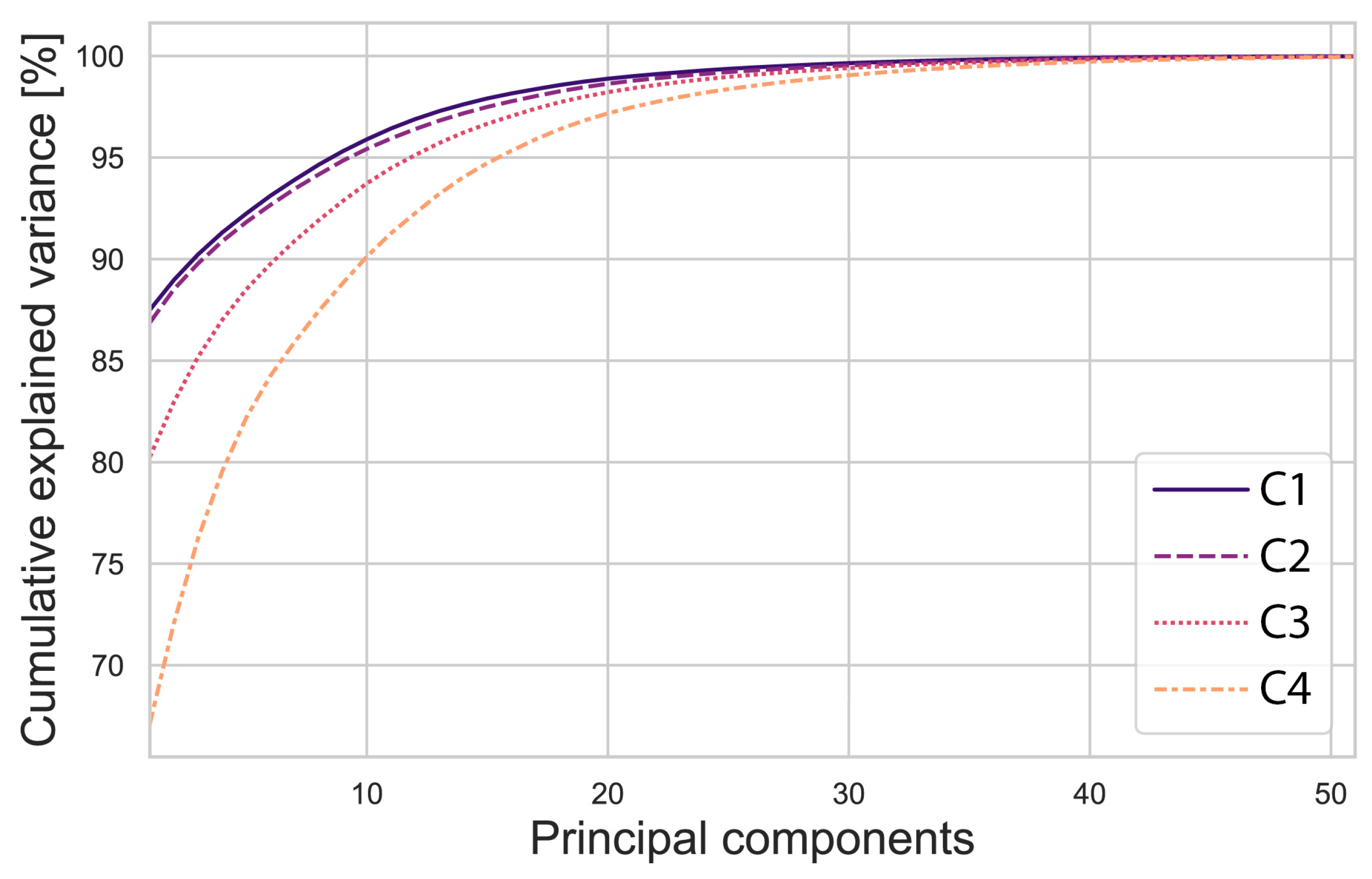
Thus, PCA was performed on the hyperspectral dataset in order to reduce the number of features per pixel and allow machine learning models to operate on a lower-dimensional feature space. In order to ensure consistency in the reduced feature set across the entire dataset, all pixel spectra from all training images were pooled to compute a global covariance matrix of the spectral data. Following standard PCA procedure, its eigenvalues and eigenvectors were determined. Specifically, eigenvectors representing linear combinations of the original spectral bands were calculated from the covariance matrix, and those associated with the largest eigenvalues were selected as principal components. The eigenvectors, acting as principal axes, corresponding to the largest eigenvalues, produce the directions of greatest variance in the data. From this analysis, it was experimentally determined that the first 51 principal components were sufficient to account for 99.99% of the total variance in our hyperspectral data. For reference, Figure 5 shows the cumulative explained variance as a function of number of principal components. As illustrated, further inclusion of additional principal components leads to an asymptotic approximation toward 100% explained variance. Thus, the number of principal components was set to $N_{\mathrm{PC}}=51$, and all hyperspectral pixel vectors were mapped from 141-dimensional to 51-dimensional feature vectors. This transformation considerably reduced data size and, most importantly, removed the multicollinearity between bands [70]. It is worth noting that the first few principal components in our transformed data captured broad spectral shape differences, such as overall reflectance level, and the slope from blue to red, which are likely related to the presence or absence of rust, whereas later components captured finer distinctions.

Following the dimensionality reduction step, two versions of the constructed dataset were prepared for classification: one with full spectral features (141 bands) and one with PCA features (51 principal components). This allowed for further performance comparison of models operating on both uncompressed and compressed measurements.

3.4. Dataset Construction and Partitioning

From the calibrated hyperspectral images, a labeled dataset of pixels for the machine learning models was constructed. Each pixel in each of the acquired images was manually assigned a class label corresponding to the corrosion level of that location (C0 through C4 as defined earlier). In order to systematically perform the labeling operation, ground truth segmentation masks were created for each image. Ground truth segmentation masks were manually created with the use of the Computer Vision Annotation Tool (CVAT) [72]. With the objective of enforcing spatial correspondence between the acquired hyperspectral images and the ground truth segmentation masks, manual annotation was performed on approximate RGB compositve images of the hyperspectral images, constructed using individual spectral bands corresponding to Red, Green and Blue wavelengths. In the RGB composite images, regions of interest were manually annotated in order to mark areas of uniform class according to the classes established in Section 3.2.

Using the annotated ground truth segmentation masks, the pixel spectra for each class were extracted. In total, tens of thousands of pixels were collected and organized according to their annotated classes in the ground truth segmentation masks for each image. The extracted spectra were then randomized and pooled these into a single dataset in order to eliminate the possibility of overfitting due to iterative machine learning model training procedures. Due to the fact that images were collected using the same setup (with uniform camera-sample distance), were the same size and each coupon had roughly equal area, the class representation in the dataset was proportional to the physical area of that class present in the samples. The painted (C0) class had contributions from three half-plates, thus it constituted the largest portion of the dataset, whereas the severe corrosion class (C4) came from one plate and was proportionally smaller in pixel count.

Table 1. Class distribution of the hyperspectral corrosion dataset and the split into training and testing sets (in percentage of total samples). C0 = no corrosion (painted), C1 = 5-day light corrosion, C2 = 10-day moderate corrosion, C3 = 15-day high corrosion, C4 = 20-day severe corrosion.

Class	Training Samples (% of Total)	Test Samples (% of Total)	Total (%)
C0 (no corrosion)	16.32%	8.26%	24.58%
C1 (5-day corrosion)	9.11%	4.51%	13.62%
C2 (10-day corrosion)	6.01%	2.98%	8.99%
C3 (15-day corrosion)	10.40%	5.05%	15.44%
C4 (20-day corrosion)	24.83%	12.53%	37.37%

summarizes the dataset distribution and the training/testing split. In order to reach this distribution, a stratified random split was employed: 2/3 of the pixels from each class were randomly selected for the training set and the remaining 1/3 for the test set. Maintaining this ratio within each class is intended in order to ensure that all corrosion levels are proportionally represented in both training and test subsets.

As expected, the severe corrosion class (C0) makes up about 37.4% of all pixels, and light corrosion (C1) about 13.62%, etc., reflecting the differing areas of those materials in the images. These percentages are also split 2:1 between training and test. In absolute terms, the dataset contained on the order of ${10}^5$ pixel samples in total (e.g., if each image has 315 k pixels and many are background or not used, the labeled count might be slightly less, but still very large for training). We did not use every single pixel to train the models (to avoid overfitting to extremely large data and to reduce training time); instead we randomly sampled a subset of pixels per class for training the models, on the order of a few thousand per class. However, for testing, we did evaluate on a large number of pixels to get robust accuracy estimates.

3.5. Machine Learning Classification Models and Evaluation Metrics

In order to provide a comprehensive evaluation of the classification performance of hyperspectral images of corroded steel samples and the differentiation of corrosion levels from spectral information, four machine learning models were evaluated: k-nearest neighbors (k-NN), support vector machine (SVM), random forest (RF), and a multilayer perceptron (MLP) neural network. These models span a range from simple instance-based learning to complex nonlinear neural-network-based learning, allowing for a varied comparison of their performance on this task.

3.5.1. k-Nearest Neighbors (k-NN)

k-NN is one of the simplest classification algorithms. It is a non-parametric, instance-based method that makes predictions based on the proximity of a sample to points in the training set [73,74]. In k-NN, a pixel’s class is determined by the majority vote of its k nearest neighbors in the feature space. For the distance metric, the standard Euclidean distance on the spectral feature vectors was selected. The value of k is a hyperparameter; common choices are small odd numbers, with the objective of avoiding ties. In our implementation, the parameters $k=3$ and $k=5$ were tested using cross-validation on a subset of the training data. It was found that $k=5$ provided slightly better accuracy than did $k=3$ for our dataset and thus was selected for the final model. This selection implies that for any hyperspectral pixel of unknown class, the model will compare the unknown pixel’s spectrum with those of the 5 most similar training pixels and assign the class by majority vote. k-NN has the advantage of being a relatively straightforward methodology that makes no assumptions about underlying data distributions. However, it suffers from impacted performance in the cases where there is significant class overlap in the feature space. Furthermore, k-NN approaches have been demonstrated to be sensitive to the local density of samples [75]. It is important to highlight that while it has no explicit training step beyond the preprocessing and organizing of data, model inference times increase in a direct proportion to the size of the training set due to the fact that unknown pixels are compared to all points in the training set in order to each a class consensus.

3.5.2. Support Vector Machine (SVM)

SVM is a powerful supervised learning algorithm that finds an optimal hyperplane to separate data points of different classes [76]. For cases where the data are not linearly separable in the original feature space, SVM uses a kernel function to implicitly map data to a higher-dimensional space where a linear separator may exist. For the purposes of this study, an SVM with the radial basis function (RBF) kernel was employed, which is a common choice for multi-spectral data [77]. The RBF kernel $K(x_i,x_j)=exp(-\gamma \parallel x_i-x_j{\parallel }^2)$ introduces a parameter $\gamma$ that controls the kernel width, which can be interpreted as a measure of the influence of a single training example. A value $\gamma =0.001$ was set based on typical values used in literature for spectra classification and some preliminary tuning. It is important to note that for the current case of multi-class classification, SVM was originally designed for binary problems. Thus, we used the one-vs-one pairwise classification strategy to handle the 5 classes. This means the classifier internally trains $\left({\displaystyle \genfrac{}{}{0pt}{}{5}{2}}\right)=10$ binary SVMs for every pair of classes and then uses a voting scheme for the final prediction. SVMs are known to perform well in high-dimensional spaces and with smaller datasets, as they are less prone to overfitting than are many flexible models [78,79]. However, they can be computationally intensive for large datasets, and tuning the kernel parameters is important.

3.5.3. Random Forest (RF)

Random forest is an ensemble learning method based on decision trees. It builds a large number of decision trees (which comprise the “forest”) and combines their outputs, typically by voting, to make a final prediction [80,81]. In this approach, each tree in the forest is trained on a random subset of the training data and with a random subset of features chosen at each split, which ensures the trees are de-correlated. RF often achieves high accuracy and is robust against overfitting due to the averaging effect of many trees [81]. Another advantage is that RF handles input features of differing scales or distributions naturally and is relatively insensitive to monotonic transformations of features. In our implementation, the number of trees was set to 100, which is usually sufficient for convergence of the ensemble’s performance [82,83]. Each decision tree split was chosen by Gini impurity minimization. Individual tree depth was not limited, which allowed them to grow until leaves were pure or contained a minimum number of samples. By ensemble averaging, the RF mitigates the risk of any single deep tree overfitting to the training data. Random forests are known to perform well even with many input features because trees will automatically select the most informative features for splits, and the ensemble can handle redundant features without much issue. In the presented experiments, RF was the most resilient model when using the full-dimensionality 141-band data, which experimentally validates the claim that it is not affected by the scale of data and can adapt to ignore irrelevant features [84].

3.5.4. Multilayer Perceptron (MLP) Neural Network

The MLP is a type of feed-forward artificial neural network. It consists of layers of individual neurons, arranged in layers: an input layer (which takes the feature vector), one or more hidden layers of interconnected neurons, and an output layer that produces class probabilities [85]. In an MLP, each neuron computes a weighted sum of its inputs and applies a non-linear activation function to the results [86]. The network is trained via backpropagation, an algorithm that adjusts the weights to minimize the classification error on the training set [87,88]. In our study, we designed a relatively small MLP appropriate for the size of our data. We used two hidden layers, each with 100 neurons, and the ReLU (rectified linear unit) activation function for these layers. The output layer had 5 neurons, corresponding to the 5 output classes, with softmax activation being applied to yield probability-like outputs. The MLP was trained using stochastic gradient descent, implemented through the Adam optimizer [89], and used categorical cross-entropy as the loss function [90]. The choice of two hidden layers was made to provide the network with the capability to capture nonlinear patterns present in the data without making the network too deep, which increases the risk of overfitting in the absence of proportionally increasing training data sizes. Key hyperparameters for the MLP included the learning rate, number of epochs, and batch size, which were tuned slightly on a validation set. Training was performed for 50 epochs, ensuring convergence of training/validation accuracy. The MLP, being a model with a fundamentally higher degree of freedom, has the potential to accurately model nonlinear relationships in the spectral data, but it also requires sufficient data and possibly regularization to generalize properly [91,92,93].

Each of the above-described models was trained on the training portion of the dataset and then applied to the test set to predict the corrosion class for each pixel. In order to evaluate the performance, two main metrics were used: the overall accuracy and the confusion matrix. Accuracy (ACC) was defined as the fraction of correct predictions out of all predictions made:

$$\mathrm{Accuracy}={\displaystyle \frac{N_{\mathrm{correct}}}{N_{\mathrm{total}}}}={\displaystyle \frac{1}{N_{\mathrm{total}}}}\sum _{i=1}^{N_{\mathrm{total}}}\mathbf{1}\{{\widehat{y}}_i=y_i\},$$

(3)

where $y_i$ is the true class of sample i, ${\widehat{y}}_i$ is the predicted class, and $\mathbf{1}\left\{\right\}$ is the indicator function (1 if the predicate is true, 0 otherwise). The accuracy metric effectively provides a direct and objective overall performance measure, but it can mask details about which classes are confused with which. For this reason, confusion matrices for each model are presented as well. The confusion matrix is a $N\times N$ arrangement, where N represents the number of classes. In a confusion matrix, the entry in the i-th row and j-th column indicates how many samples of true class i were predicted as class j. From the confusion matrix, per-class accuracy, therefore sensitivity and recall, can be derived. Most importantly, it allows for the determination of pairs of classes that are commonly classified incorrectly as either.

4. Results and Discussion

In this section, we present the performance results of the four classification models on the hyperspectral corrosion dataset and provide a comparative discussion. We evaluate model accuracy with and without PCA-based dimensionality reduction, analyze the confusion matrices to understand misclassification patterns, and discuss the practical implications in terms of the advantages and drawbacks of each approach.

4.1. Classification Performance with PCA Features

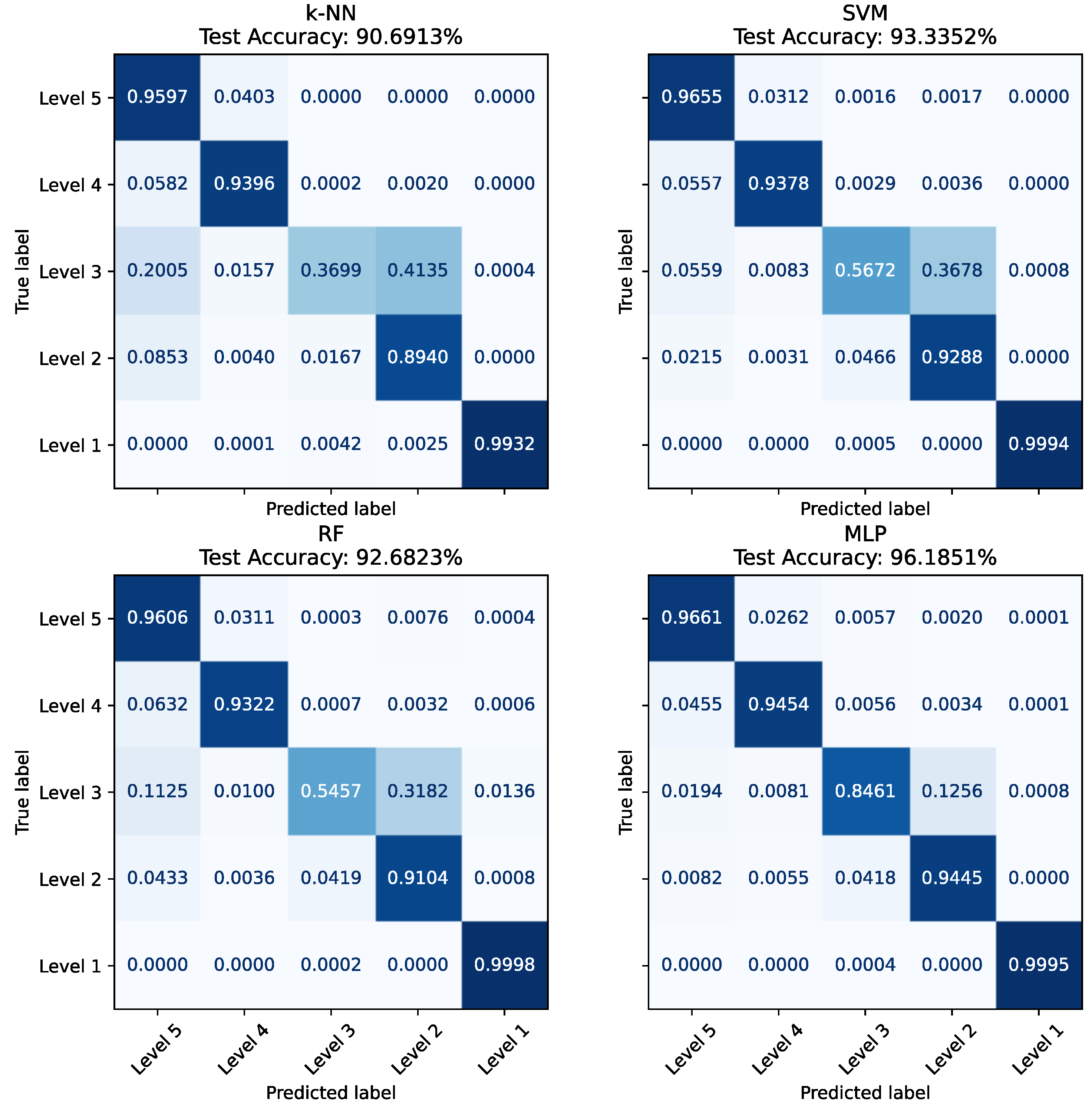
After reducing the hyperspectral data to 51 principal components according to the procedure outlined in Section 3.3, we trained and tested the k-NN, SVM, RF, and MLP models as described. All models achieved high overall accuracy on the test set, indicating that the spectral information captured by HSI is verifiably discriminative for corrosion level identification. Of the evaluated models, MLP yielded the highest accuracy among the four. For reference, the normalized confusion matrices for each model, using PCA features, are shown in Figure 6. The overall test accuracies were as follows: MLP = 96.18%, SVM = 93.33%, RF = 92.68%, and k-NN = 90.69%. The MLP correctly classified about 96% of all pixels in the test set, the highest of the evaluated models for the current five-class problem. The second-highest accuracy was achieved by SVM, which produced results with 2.85% less accuracy, followed closely by RF. The k-NN model produced the least accurate results.

These results demonstrate that with appropriate dimensionality reduction preprocessing using PCA and an appropriate model, hyperspectral imaging can distinguish different corrosion levels with high accuracy. All models substantially outperformed random guessing, which would be 20% accuracy for a five-class problem, as well as the expected results from a binary corroded vs. not corroded classifier model. The obtained results suggest that the spectral signatures in corroded steel coupons provide enough underlying information for corrosion grade classification at an acceptable level even while using simpler models such as k-NN.

A close inspection of the confusion matrices in Figure 6 confirms that Class (C0), which represents the painted and non-rusted surface, was almost perfectly recognized by every model. This finding is congruent with Figure 4, where the C0 spectra stand apart from those of all corrosion classes. Every classifier achieved true-positive rates above 95 percent for C0, so virtually every painted pixel was accurately classified as non-corroded. The paint reflectance spectrum is therefore clearly distinguishable from any corroded-steel spectrum, as previously recognized. However, the situation is less straightforward for the corroded categories C1 to C4, which span light through severe corrosion. Spectral overlap between neighboring levels produced classification inconsistencies, and the light corrosion (C1) and moderate corrosion (C2) cases were the most frequently confused. The k-NN classifier showed the highest performance impact, and its true-positive rate for C1 dropped because some C1 pixels were predicted as C2, and a smaller portion were even mapped to C0. A plausible explanation is that a five-day exposure to the corrosion medium can yield spectra that remain similar to those obtained after ten days, while very lightly corroded locations inside C1 can still exhibit reflectance values that sit closer to paint than to rust. The severe corrosion class C4, produced after twenty days of exposure, was identified accurately by almost every model. This class is spectrally homogeneous, as the entire steel plate is covered by oxide, and the lower overall reflectance associated with the darker surface improves its statistical separability from the lighter classes. Consequently, all algorithms labeled more than 95 percent of the C4 pixels correctly, with k-NN having the lowest performance in the ensemble while still assigning the majority of C4 test classifications properly.

Inspection of the k-NN confusion matrix indicates that its largest errors centered on C1 and C2. The method relies on local distances in feature space, so two neighboring classes that are spectrally close can mislead the vote. If the difference between ten-day and fifteen-day spectra is small, a pixel from the latter may locate nearest neighbors that belong to the former and will inherit their label. On the other hand, the MLP and SVM generated confusion matrices that were almost diagonal. The MLP exhibited consistently high true-positive rates across all classes. When mistakes occurred, they predominantly involved swapping C1 and C2 and, to a lesser extent, C2 and C3. The SVM followed the same pattern although its accuracy on C2 was appreciably lower. The RF algorithm presented a similarly balanced performance profile. However, its recognition of C2 lagged behind that of the multilayer perceptron, while it matched the neural network and the support vector machine in every other class. This outcome highlights the general robustness of the ensemble method.

From these results, a clear outcome is that a dimensionality reduction step allows all models to distinguish corroded from non-corroded areas with a high degree of accuracy, in addition to further differentiating the various degrees of corrosion with considerable success. The relatively small performance gap between SVM, RF, and MLP suggests that the choice of model can be guided by other considerations, such as convenience or compute availability. However, the MLP’s top accuracy points to the potential of deep learning to capture subtle nonlinear patterns in the data that the other models might not fully exploit.

It is also worth noting that none of the models showed any systematic bias toward classifying everything as one of the majority classes. All confusion matrices had strong diagonal values for each class rather than only the large class, indicating that all classes were adequately generalized by the models. This is an increasingly important concern as dataset sizes grow, as large class imbalances can lead to a situation where models optimize for maximizing discriminative capacity for the largest class to the detriment of the others.

4.2. Dimensionality Reduction Considerations

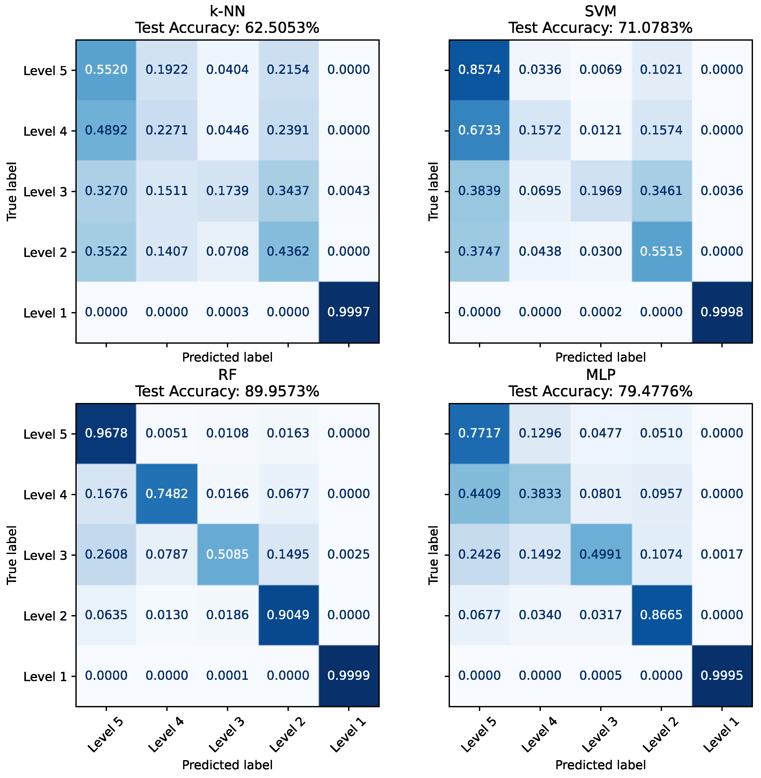
In addition to the results summarized in Figure 6, model performance was evaluated when trained with full-dimensionality spectral data without a PCA-based dimensionality reduction step. In theory, more features could provide more information but could also increase the required model complexity and the risks of overfitting and lack of adequate convergence due to the high-dimensionality feature spaces involved. The summarized model performance results are presented in the form of confusion matrices for reference in Figure 7. For the full-dimensionality experiment, the highest performing model was the RF, which presented a classification accuracy of 89.96% on the testing set. Following this, in descending order, were MLP (79.48%), SVM (71.08%), and k-NN (62.50%). The results of these experiments validate the positive influence of a dimensionality reduction preprocessing step on model classification performance. It is important to note that despite being an iterative model with less fundamental complexity than its MLP and SVM counterparts, the RF algorithm exhibited a superior robustness in extracting accurate classification results when using the full-dimensionality spectral data. K-NN performance was largely unchanged and still produced the least accurate results. However, the k-NN accuracy results indicate a higher proportional drop in performance compared to those of its counterparts. This highlights the established impact of high-dimensional data on the accuracy of distance-metric-based models according to the curse of dimensionality [57,58]. Furthermore, in this experiment, the SVM’s kernel and margin optimization were required to consider a feature space with 141 dimensions, significantly impacting computational complexity and potentially introducing many support vectors representing statistical noise. The MLP, if provided with all 141 inputs during training, is required to adaptively learn the relevant spectral linear combinations required for accurate classification among a higher proportion of noisy or irrelevant features.

On the other hand, the RF model proved to be relatively immune to irrelevant or highly redundant features common in spectral measurements compared to its counterparts. This is because each tree can pick only the useful features for its splits and having more features (even if some are correlated) does not reduce the classification performance of the trees.

In the examination of the confusion matrices for the full-band models in Figure 7, it is important to note that the SVM and k-NN present significant confusion statistics among the classes associated with corrosion spectral measurements. In this regard, both methodologies do not present a clear diagonal majority in their confusion matrices, leading to the conclusion that they misclassified more spectra for each corrosion level than they classified accurately. In a similar manner to the trends observed in Section 4.1, the statistical separability of C0 class spectra from the C1, C2, C3, and C4 class spectra is high, leading to classification accuracies above 99% for this class in all the evaluated models.

One important practical consideration is how these models respond to outliers or unusual conditions. Hyperspectral data can sometimes contain outlier spectra from a variety of sources not present in training data, such as localized noise spikes, specular reflections, and uneven illumination and shading. Due to practical considerations, it is not feasible to assume that hyperspectral sampling will always be performed in the absence of operational conditions that lead to these outliers. For this reason, robust preprocessing steps, such as intensity, thresholding, or statistical filtering for outlier removal could aid in the improvement of the consistency of classification performance of all models.

4.3. Advantages of HSI for Corrosion Inspection

The favorable classification performance across all evaluated models described in Figure 6 confirms that hyperspectral imaging in the visible-to-near-infrared range is a viable technology for corrosion degree evaluation in marine ship vessels. In the dimensionally reduced experiment, optimal for implementation in terms of both classification performance and computational complexity, the lowest performing model could correctly classify over 84% of pixels into the correct corrosion level, and the highest performing model presented a classification accuracy above 96%. These accuracy figures highlight the promise of the technology for this application given that visual discrimination by a human operator of corrosion degrees can be highly subjective without the use of proper measuring tools and spatial positioning. Another advantage is that HSI, being a non-contact, non-destructive optical method, can cover large areas at a fine spatial resolution depending on specific sensor specifications. Unlike point measurements, such as ultrasonic or electrical resistance probes, HSI produces a continuous surface condition map of the surface condition. This allows for the identification of hotspots of severe corrosion, the mapping out of areas needing repair, and the ability to distinguish them from lightly affected areas.

However, our study also revealed some limitations and considerations. First, the spectral difference between different grades of rust was not extremely large (unlike, for instance, the differences between bare metal and rust or between paint and rust). This means that while HSI can separate these classes with ML assistance, it is not a trivial task, and there exists a constant possibility of localized misclassifications. In addition, field conditions may introduce variations (lighting changes, shadows, specular reflections, dust or biofouling on surfaces, different paint types, etc.) that could affect the spectral readings. To mitigate this, proper illumination calibration methodologies are imperative to obtain accurate, consistent results. In addition, training sets can be complimented with field measurements to obtain a higher range of the spectral variability of evaluated materials.

In terms of practical deployment, recently developed HSI cameras in the visible/NIR range are relatively compact and can be seamlessly mounted on drones or cranes. However, they do require stable, broadband lighting or their own light source for consistent results [94,95]. Furthermore, since hyperspectral data can be reinterpreted post-collection, the same data could be used for other analyses, such as identifying if the corrosion is mostly general surface rust or if there are signs of pitting, which could be identified with the use of spatiospectral hyperspectral image-processing approaches [96,97].

5. Conclusions

This work demonstrates the feasibility and effectiveness of hyperspectral imaging combined with machine learning for the non-destructive inspection of corrosion on steel surfaces in marine environments. Through a series of experiments on steel samples with varying corrosion exposure, we showed that HSI data can be used to accurately classify the degree of corrosion, from intact protected metal to severely rusted metal. Among the models tested, a neural network (MLP) achieved the highest classification accuracy (96.18%), closely followed by support vector machine and random forest classifiers (93.33% and 92.68%, respectively). These results are markedly superior to those that what would be achievable with conventional RGB imaging, highlighting that the rich spectral information contained in hyperspectral images are able to provide superior discrimination of corrosion states.

The high performance of the models, especially after PCA preprocessing for dimensionality reduction, confirms that spectral differences corresponding to different rust levels (e.g., thickness or composition of oxide layers) are present and can be learned. In practical terms, this means HSI can detect not just the presence of corrosion but also gauge its severity in a single imaging step. This capability can significantly aid maintenance planning for ships and offshore structures: critical heavily corroded spots can be flagged for immediate repair, while lightly corroded areas can be monitored over time and directly targeted during subsequent inspection opportunities. The non-contact nature of HSI allows inspections to be done remotely, reducing the need for personnel to perform dangerous close-up inspections on hulls or in tanks. By deploying HSI on mobile platforms, such as drones or crawler robots, integrated corrosion surveying systems could cover an the totality of the surface of a marine vessel in a fraction of the time required for manual inspection, producing digital results that can be archived and compared over successive surveys.

The current study demonstrated that HSI is viable under realistic conditions, with brackish waters from the Panama Canal being used as a corrosion medium. However, before HSI can be adopted in industry practice, there are a few considerations and future improvements to address. Firstly, the dataset acquired for the current work was constructed from hyperspectral images captured in controlled laboratory conditions. In the field, lighting variations can affect spectral measurements. Future work on this subject should evaluate the robustness of the HSI approach under varied lighting conditions or incorporate adaptive methods to correct for illumination differences [98,99]. In addition, outdoor HSI might need higher dynamic range sensors to deal with drastically different illumination conditions depending on the weather and the orientation or position of targets of interest. Further, detailed chemical analysis could be performed on steel coupons exposed to corrosion media in order to determine their exact spectral composition. This could be further validated using spectral unmixing methodologies for compositional analysis [100,101]. Further, the brackish corrosion medium evaluated in this study was extracted from the Balboa region coastline alongside the Panama Canal. Further developments on the proposed methodology should incorporate a thorough evaluation of the corrosion level classification performance for samples exposed to a wider variety of water quality parameters, such as standardized artificial seawater, open-ocean seawater, and various pollutants commonly present in marine and port environments, due to the established fact that there exists a correlation between the specific pollutant exposure and the presence of various surface corrosion products on steel surfaces, which can introduce the measured spectra of corroded steel samples [2,102,103]. Further, detailed chemical analyses of corrosion products imaged under various water composition scenarios should be pursued in order to determine exact product-specific spectral measurements. Such analyses could further validate corrosion product identification through spectral unmixing methodologies.

As HSI technology continues to mature and become more accessible, we anticipate its integration into the regular maintenance workflow for marine vessels, offshore platforms, and other critical steel infrastructures. Future developments addressing the aforementioned areas will further lay various developmental, computational, and procedural frameworks for HSI to transition from the laboratory to the dry dock, effectively contributing to safer and more efficient assessment and correction of marine corrosion.