Predicting UV-Vis Spectra of Benzothio/Dithiophene Polymers for Photodetectors by Machine-Learning-Assisted Computational Studies

Abstract

The current study represents a machine-learning (ML)-assisted reverse polymer engineering for the rational design of high-performance benzothiophene (BT) benzodithiophene (BDT) polymers for photodetector applications. By integrating their 5617 units with various acceptor moieties, a total of 72,976 unique polymer combinations are generated. The optical properties of these polymers are predicted with high accuracy (R² = 0.86) using a Gradient-Boosting Regression (GBR) model. The SHAP value-based feature importance analysis indicates that Chi0 is the most influential factor in predicting the absorption maxima (λ_max) of polymers, followed by LabuteASA, Chi0V, Chi1, SlogP_VSA12, and other molecular descriptors. The robustness of the employed model is further validated through K-Fold cross-validation, with the highest mean squared error (MSE) observed at 2.02 in the fold-2 subset. The designed polymers exhibit λ_max within the range of 400–750 nm, demonstrating their suitability for photodetector applications. Moreover, a Transformer-Assisted Orientation (TAO) approach is employed to optimize polymer design, successfully achieving bandgaps as low as 0.42 eV. This approach facilitates the rapid design and optimization of high-performance polymers with tailored electronic properties, effectively addressing the limitations of conventional trial-and-error methods. The current ML-assisted approach presents a promising strategy for expediting the development of high-performance photodetectors and other advanced optoelectronic devices.

1. Introduction

Polymeric photodetectors play a vital role in light-harvesting applications, owing to their exceptional properties that facilitate the efficient conversion of light into electrical signals [1]. These materials are typically flexible, lightweight, and easily processable into diverse shapes and sizes, enabling innovative designs for applications in imaging systems, solar energy conversion, and environmental monitoring [2]. The ability of polymeric materials to absorb across a wide spectrum becomes more efficient for solar energy capture, particularly when engineered with specific polymer structures and compositions [3]. Additionally, the fabrication of polymeric photodetectors uses cost-effective techniques like roll-to-roll printing, making them highly advantageous for large-scale production [4]. Furthermore, incorporating organic materials enables the development of devices that exhibit greater environmental suitability than their inorganic counterparts [5]. With continuous progress in the synthesis and characterization of conductive polymers and their composites, the development of high-performance polymeric photodetectors is fostering next-generation light-harvesting technologies, contributing to energy sustainability and enhanced performance across diverse applications [6]. Polymeric photodetectors offer several advantages, including tunable electronic characteristics that can be tailored through chemical modifications, cost-effective fabrication techniques such as spray coating and inkjet printing, and the potential to hybridize with nanomaterials, thereby improving efficiency and expanding spectral response [7]. Their intrinsic mechanical resilience and flexibility render them highly suitable for applications in wearable technologies and outdoor environments. Moreover, the emergence of smart materials capable of dynamically responding to external stimuli presents promising opportunities for innovations in sensing and energy-harvesting technologies [8]. The strategic design of new polymers with tailored UV-Vis spectra play a crucial role in enhancing the performance of solar cells, as it facilitates the optimization of light absorption across the solar spectrum [9].

By strategically modifying the optical and electronic properties of polymers, researchers can design materials that efficiently absorb specific wavelengths of light, thereby optimizing solar energy harvesting [10]. This optimization process often involves the utilization of different functional groups, precise control of polymer chain length, or the strategic blending of multiple polymers to attain the desired spectral properties [11]. Enhanced light absorption leads to higher photocurrent generation, which consequently improves the overall efficiency of solar cells. Additionally, polymers engineered to absorb a broader spectrum of wavelengths enable the efficient capture of both direct and diffuse sunlight, enhancing the performance efficiency of solar cells under varying environmental conditions [12]. Ultimately, the precise tuning of UV-Vis spectra in polymeric materials not only drives the advancement in high-performance solar cells but also contributes to the scalability and seamless integration of organic photovoltaic technology within a more sustainable energy framework [13]. The benzothiophene (BT) based organic polymers have gained significant attention for solar cell applications owing to their superior optical and electronic properties [14]. The unique structural framework of benzothiophene, characterized by a fused thiophene ring, facilitates high charge carrier mobility and enhances light absorption capabilities across the UV-Vis spectrum [15]. This structural attribute allows for the development of materials with precisely tuned bandgaps, optimizing the absorption of specific wavelengths, including those in the visible spectrum, to enhance solar energy harvesting efficiency [16]. Additionally, the inclusion of benzothiophene units improves the thermal stability and mechanical flexibility of the resulting polymers, ensuring their suitability for a wide range of photovoltaic applications [17]. The further engineering of these polymers by copolymerization or blending with other organic semiconductors enhances their overall performance, driving the development of cost-effective and efficient organic solar cells capable of competing with traditional silicon-based technologies [18].

The application of ML in polymer design represents a groundbreaking approach that significantly accelerates the discovery and optimization process of novel materials [19]. By analyzing extensive datasets of existing polymer properties and performance, ML-related knowledge graph algorithms can uncover hidden patterns and correlations that may not be readily evident to researchers [20]. This approach facilitates the prediction of polymer behavior based on their chemical structure and composition, enabling the rapid screening of potential candidates for applications in photovoltaics, sensors, and biomaterials [21]. The ML can also assist in the optimization of molecular structures to achieve desired properties, such as enhanced strength, electrical conductivity, or thermal stability, ultimately streamlining the design process and minimizing the time and cost associated with conventional trial-and-error experimentation [22]. The current study aims to employ ML techniques to establish a robust framework that can facilitate the development of novel polymers with tailored properties, particularly for advanced applications in energy harvesting and sustainable technologies (Figure 1). By leveraging predictive models derived from an extensive database of polymeric materials, this research seeks to identify and synthesize high-performance candidates that meet specific requirements, thus driving advancements in polymer science and tackling crucial challenges in the field of renewable energy.

2. Theory and Principle

For current work, a particular class of neural networks called Graph Neural Networks (GNNs) was exclusively designed to operate on graph-structured data [23]. Such developed models can capture the underlying properties and structure of the graph by leveraging the relationships and interactions between nodes (representing atoms or molecular fragments) and edges (representing bonds) [24]. Several crucial steps are involved in the process of implementing GNNs in the context of reverse polymer engineering. Assuming the current work, a graph can be used to represent each polymer as follows (Equation (1)).

$$G=(E, V)$$

(1)

where the sets E and V can be their nodes (atoms) and edges (bonds), respectively. Features like atom type and hybridization can also be assigned to each node as vi, while features like bond type (w_ij) can be assigned to each edge (e_ij).

For these GNNs, the message-passing mechanism can serve as their core operation, where nodes gather information from their neighbors. The message passing could be mathematically expressed as follows (Equation (2)):

$${h_i^{\left(k\right)}=\sigma (W}^{\left(k\right)}.\mathrm{A}\mathrm{g}\mathrm{g}\mathrm{e}\mathrm{r}\mathrm{g}\mathrm{a}\mathrm{t}\mathrm{e} \left(\left\{h_j^{\left(k-1\right)}:j ϵ N\left(i\right)\right\}\right)+b_i^{\left(k\right)})$$

(2)

Here, hi(k) represents the hidden state of node i at layer k, N(i) denotes the set of neighboring nodes, W(k) is the weight matrix for layer k, b(k) is their bias term, and σ is their non-linear activation function (e.g., ReLU). Once the messages are aggregated from neighbors, each node can be updated for its state according to the collected information. By repeating this process across multiple layers, nodes can gather their information from more distant areas of the graph. A pooling operation can be applied to their node attributes to obtain a graph-level representation. This was accomplished using methods such as max pooling, mean pooling, or attenuation mechanisms (Equation (3)).

$$h_G=Pooling \left(\right\{h_i^{\left(k\right)}:i ϵ V\left\}\right)$$

(3)

where K denotes the final layer of the GNN. After that, the final graph representation hGh is passed into a fully connected layer to forecast the desired characteristics, such as the band gap of the polymer (Equation (4)):

$$y=W_{out}.h_G+b_{out}$$

(4)

where y is the predicted output, and W_out and b_out are the weights and bias of the output layer. In the context of Gaussian processes [25], particularly in the field of spectroscopy or photophysics, the absorption and emission maxima (λ_max and λ_E) of a material can be derived from the spectral data obtained through Gaussian fitting. Here’s a general outline of how a Gaussian function can be expressed as:

$$\int \left({\mathit{f}}_{\mathit{x}}\right)=\mathit{A}.{\mathit{e}}^{-{\displaystyle \frac{{(\mathit{x}-\mathit{\mu })}^2}{{2\mathsf{\sigma }}^2}}}$$

(5)

where f(x) is the intensity at position x. A is the amplitude (peak height). μ is the mean (the position of the peak, which corresponds to the maximum). σ is the standard deviation (related to the width of the peak).

Their λ_max can be found by fitting the absorption spectrum data to a Gaussian function [26]. The position of the peak μ from the fitted Gaussian function corresponds to the λ_max. Similarly, for emission spectra, the λ_E can also be determined by fitting the emission spectrum data to a Gaussian function. Again, the position of the peak μ from the fitted Gaussian function corresponds to the λ_E. To calculate emission spectra using Gaussian processes (GP), we typically start with a set of descriptors that characterize the system or material of interest. These descriptors can include various physical and chemical properties, such as molecular structure, electronic states, or environmental factors. The Gaussian process can then be used to model the relationship between these descriptors and the emission spectra.

2.1. Step-by-Step Approach

Define the descriptors xx that will be used to predict the emission spectra. These could be vectors representing various features of the system. The Gaussian process is defined by a mean function and a covariance function (kernel). The general form of a Gaussian process can be expressed as (Equation (6)):

$$k\left(x,{\mathrm{x}}^{\mathrm{\prime }}\right)={\sigma }_f^{2}exp(-{\displaystyle \frac{{\mid \mid \mathrm{x}-\mathrm{x}\mathrm{\prime }\mid \mid }^2}{{2l}^2}})$$

(6)

where σ²_f is the variance (signal variance), and l is the length scale, which controls how quickly the correlation between points decreases with distance (Equation (7)).

$$\left[{\displaystyle \genfrac{}{}{0pt}{}{y_{*}}{y_{*}^{*}}}\right]~N\left(\left[{\displaystyle \genfrac{}{}{0pt}{}{{m\left(x\right)}_{*}}{{m\left(x\right)}_{*}}}\right],\left[{\displaystyle \genfrac{}{}{0pt}{}{{K(x}_{*},x_{*})}{K(x,x_{*})}}{\displaystyle \genfrac{}{}{0pt}{}{{ K(x}_{*},x)}{ K(x,x)}}\right]\right)$$

(7)

where K(x*,x*) is the covariance matrix for the new inputs. K(x*,x) is the covariance between the new inputs and the training inputs. K(x,x) is the covariance matrix for the training inputs. The predicted mean y∗y∗ will give the expected emission spectra for the new descriptors x*x*. The variance can also be used to quantify the uncertainty in the predictions.

2.2. Data Collection

The methodology to utilize ML approaches for analyzing a large dataset of benzothio- and dithiophene-based compounds involved various systematic steps, which started from data collection, descriptor designing, descriptor designing, model training, and evaluation. A comprehensive dataset consisting of 5617 relevant compounds was assembled from various chemical databases, including a majority from PubChem. The dataset was processed to eliminate missing entries, duplicates, and unnecessary compounds (Figure 2).

2.3. Descriptor Designing

Molecular descriptors were calculated for each compound to capture pertinent structural and electronic attributes. Typical descriptors included (Equation (8)).

$$MW={\sum }_{i=1}^n{m}_i$$

(8)

where mi was the atomic mass of atom i in the molecule.

Similarly, their partition coefficient (LogP) is used to calculate the octanol–water partition coefficient, which is a measure of the distribution of a chemical compound between two immiscible phases (Equation (9)). Its high LogP value shows that a compound is more soluble in lipophilic (octanol), while its low LogP value indicates that it is more soluble in hydrophilic media (water).

$$LogP={Log}_{10}\left({\displaystyle \frac{C_{octanol}}{C_{water}}}\right)$$

(9)

As follows is the Wiener index, where dij represents the distance between nodes i and j in the molecular graph (Equation (10)).

$$W={\sum }_{i=1}^n{\sum }_{j=1}^n{d}_{ij}$$

(10)

where χi denotes the electronegativity of atom i (Equation (11)).

$$EN={\displaystyle \frac{1}{n}} {\sum }_{i=1}^n{x}_i$$

(11)

For their molecular valence connectivity indices (${\chi }_{\mathrm{n}}^{\mathrm{v}}$) [27], their calculations were performed by assuming their hydrogen-suppressed skeletons along with (Equation (12)) their non-hydrogen atom to have their unique δv value as denoted by their atomic valence delta (δ^v).

$$(\mathrm{For} \mathrm{zero-order} \mathrm{connectivity}) {\chi }_{\mathrm{o}}^{\mathrm{v}}={\sum }_{\mathrm{i}=10}^{\mathrm{n}}{\left({\delta }^{\mathrm{v}}\right)}^{-0.6}$$

(12)

For this, their δ^v was calculated from their atomic numbers (Z) and valence electrons (Z^v) along with their attached hydrogen atoms (h) (Equation (13)).

$$\delta ={\displaystyle \frac{{\mathrm{Z}}^{\mathrm{h}}-\mathrm{h}}{\mathrm{Z}-{\mathrm{Z}}^{\mathrm{h}}-1}}$$

(13)

3. Results and Discussion

3.1. Descriptor Correlations

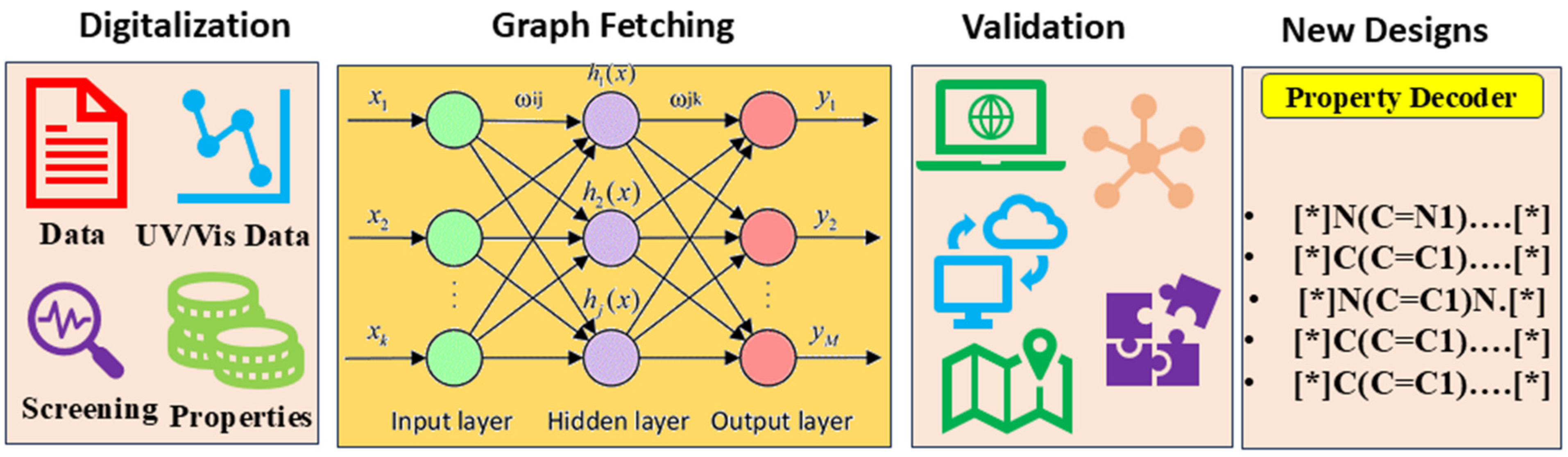
The integration of ML into polymer design has led to a significant transformation, drastically revolutionizing the discovery and optimization process [19]. By leveraging vast repositories of polymer properties and performance data, ML algorithms can uncover hidden patterns and correlations that might have been overlooked by human researchers [28]. This enables the precise prediction of polymer behavior based on chemical structure and composition, facilitating the rapid screening of potential candidates for specific applications, including sensors, photovoltaics, and biomaterials [29]. Moreover, ML can facilitate the optimization of molecular structures to achieve desired properties, such as improved strength, thermal stability, and electrical conductivity, thus streamlining the design process and reducing the time and cost involved in trial-and-error experimentation. The top-performing tokens underwent regression analysis across various graph neural network models, yielding promising outcomes. Specifically, the Aromatic Carbonyls token attained an impressive R² value of 0.91 and a low RMSE value of 0.0021 when assessed using a Random Forest model (

Table 1. A view of the highly accurate ML model to predict the data structure of the designed tokens of the collected dataset.

Token	Model	R2	RMSE
Aromatic_Carbonyls	Random Forest	0.91	0.0021
Aromatic_Heterocycles	Decision Tree	0.92	0.0032
Aromatic_Rings	Random Forest	0.89	0.0029
HAcceptors	Decision Tree	0.87	0.0018
HeteroAtoms	xGBoost	0.79	0.0009
RotabaleBonds	Gradient Boosting	0.82	0.0031
RingCount	Random Forest	0.83	0.0021
Fr_Benzene	Random Forest	0.86	0.0160
Fr_Bicyclic	Decision Tree	0.83	0.0150
Fr_Ether	Random Forest	0.79	0.0140
Fr_thiophene	Random Forest	0.85	0.0120

).

The Aromatic_Heterocycles token exhibited even superior performance, achieving an R² value of 0.92 and an RMSE value of 0.0032 when evaluated using a Decision Tree model. The Aromatic_Rings token also showed robust correlations, yielding an R² value of 0.89 and an RMSE of 0.0029 when analyzed using the Random Forest model. Meanwhile, the HAcceptors token demonstrated a strong correlation, with an R² value of 0.87 and an RMSE of 0.0018 when evaluated using the Decision Tree model. The HeteroAtoms token, however, exhibited the best fit with the xGBoost model, attaining an R² value of 0.79 and an RMSE of 0.0009. The Rotatable Bonds token displayed moderate predictive performance, achieving an R² value of 0.82 and an RMSE of 0.0031 when implemented using the Gradient-Boosting model. The Ring Count token showed comparable results, with an R² value of 0.83 and an RMSE of 0.0021 when analyzed using the Random Forest model. The Fr_Benzene token exhibited strong performance, with an R² value of 0.86 and an RMSE of 0.016 with the Random Forest model. In contrast, the Fr_Bicyclic token achieved an R² value of 0.83 and an RMSE of 0.015 when utilizing the Decision Tree model. Finally, the Fr-ether and Fr_thiophene tokens exhibited moderate to strong predictive performance, attaining R² values of 0.79 and 0.85, respectively, when applying Random Forest models.

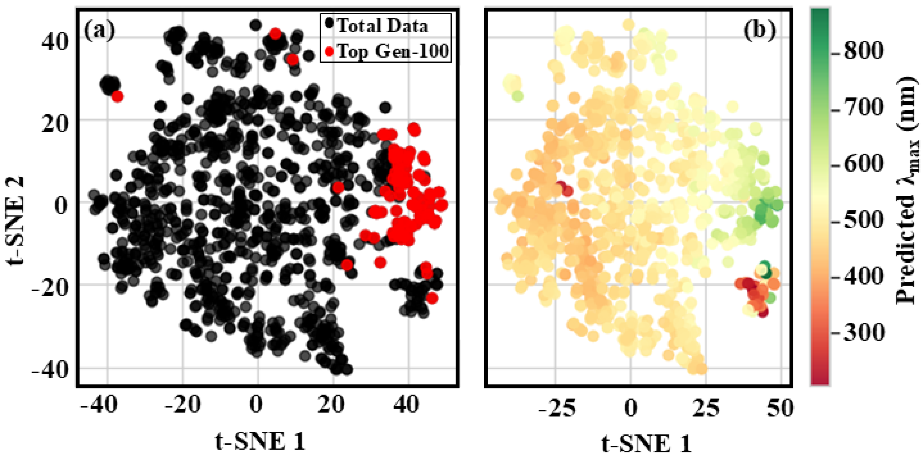
The t-SNE map constructed using these descriptors provided significant insights into the distribution patterns of the training and generation-1 datasets. The map illustrated a broad distribution of data points across both tSNE-1 and component 2, with tSNE-1 ranging from −50 to 50 and component 2 spanning from −80 to 80 (Figure 3). Notably, the data points corresponding to both the actual and ground-predicted results were uniformly distributed across the map, highlighting a strong congruence between them. The uniform distribution of data points suggested that descriptors employed in this analysis effectively captured the intrinsic patterns and relationships within the dataset. This observation held particular significance, as it suggested that the model had effectively acquired meaningful representations of the data, exhibiting a strong correspondence with its inherent structural framework. The dispersion of data points across the entire map, rather than their concentration in a specific region, suggested that the model had successfully captured a comprehensive and diverse set of features, effectively representing the intrinsic properties of the polymer. Furthermore, the t-SNE map offered a visual depiction of the high-dimensional data, facilitating a more intuitive exploration and in-depth analysis of the relationships among various data points. The nearly uniform distribution of data points between the actual and ground-predicted results suggested that the model had effectively generalized to new, unseen data rather than merely memorizing the training instances.

This finding provided a compelling indication of the model with its capability to generate accurate predictions for new, unseen data, emphasizing the potential of this approach in expediting the design and discovery of new polymers with tailored properties.

Beyond its impressive performance in predicting polymer properties, the synthetic feasibility of the generated polymers remained a critical factor for consideration. The synthetic accessibility metrics, ranging from 0.001–0.20, provided crucial insights into the feasibility of synthesizing these designed polymers within a laboratory environment. Notably, the majority of the data points displayed the highest density around a synthetic accessibility value of 0.05, suggesting that most of the designed polymers possessed moderate to high synthetic feasibility. This finding was particularly promising, as it suggested that a substantial proportion of the generated polymers were realistically synthesizable using contemporary laboratory methodologies and available resources. The high density of data points around 0.05 further suggested that the model had successfully generated polymers that were not only optimized for their predicted properties but also accounted for the practical considerations of their synthesis. This aspect was fundamental to any materials design endeavor, as accurately predicting a material with its properties was only one part of the challenge; ensuring its practical feasibility for synthesis and characterization was equally essential. The broad range of synthetic accessibility values, spanning from 0.001–0.20, further underscored the structural diversity of the generated polymers. While certain polymers may pose greater challenges in synthesis, others may be more readily obtainable. Its capacity to generate a diverse range of polymers with varying synthetic accessibility values could offer researchers a broader spectrum of potential opportunities to pursue.

3.2. Predicting λ_max

In predicting the λ_max of a particular phenomenon, various regression models exhibited varying degrees of performance. An analysis of the results revealed that the Gradient-Boosting model stood out as the most effective, achieving a notable R² value of 0.86 and an exceptionally low RMSE of 0.0021. This showed that the model effectively captured the underlying patterns in the data with a high level of accuracy [30]. In comparison, AdaBoost performed slightly less effectively, yielding an R² value of 0.81 and an RMSE of 0.0430 (

Table 2. Model evaluation results of the evaluated ML models to predict their maximum absorption spectra.

Model	R2	RMSE
Gradient Boosting	0.86	0.0021
AdaBoost	0.81	0.0430
K-Nearest Neighbor	0.67	0.0051
Decision Tree	0.71	0.0009
xGBoost	0.76	0.0022
LightGBM	0.69	0.0041

). Although still commendable, these metrics indicated that the model was comparatively less effective in predictive performance.

The K-Nearest Neighbor model exhibited an even lower performance, achieving an R² value of 0.67 and an RMSE of 0.0051. This model struggled to capture the intricate patterns within the data, resulting in reduced predictive accuracy. The Decision Tree model demonstrated moderate performance, attaining an R² value of 0.71 and an RMSE of 0.0009. Meanwhile, the xGBoost and LightGBM models exhibited moderate performance, yielding R² values of 0.76 and 0.69, respectively, with corresponding RMSE values of 0.0022 and 0.0041. Notably, the differences in performance among these models could stem from various factors, including data complexity, the extent of hyperparameter tuning, and the specific nature of the phenomenon being predicted.

3.3. Regression Analysis

The Gradient-Boosting Regression analysis, which achieved an impressive R² value of 0.86 and an RMSE of 0.002, represented a noteworthy accomplishment. This algorithm integrated multiple weak models to construct a robust predictive model, which, in this case, was employed for regression analysis to estimate continuous values. The model performance was likely optimized through hyperparameter tuning, taking into account key factors such as the number of estimators, learning rate, maximum depth, and minimum sample size. Furthermore, feature engineering played a pivotal role in identifying and transforming the most relevant attributes from the dataset, ultimately improving its overall performance. This process likely encompassed handling missing values, feature scaling, and selecting relevant features through techniques such as mutual information, correlation analysis, or recursive feature elimination. 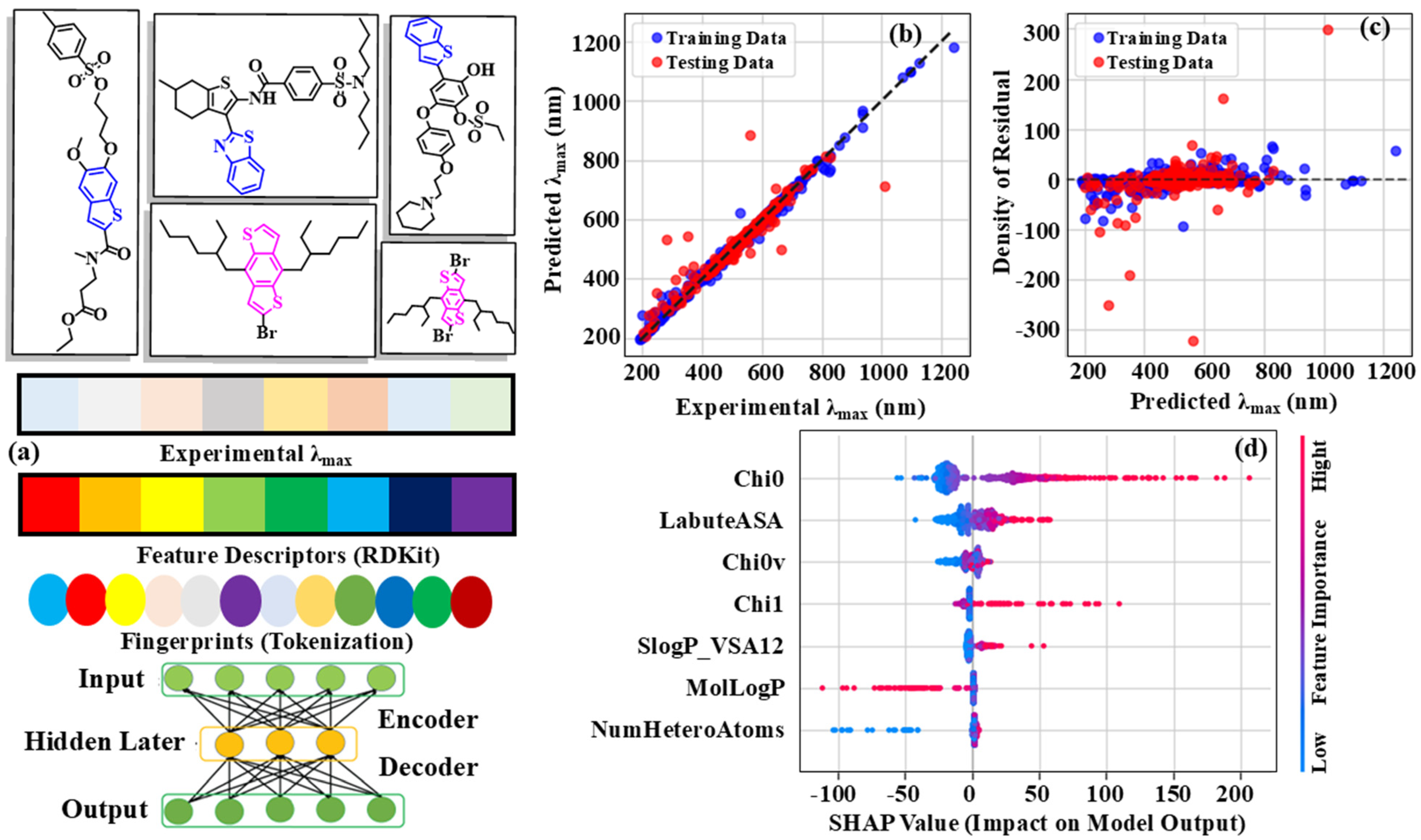The model performance was evaluated based on R² and RMSE metrics, offering valuable insight into its effectiveness in capturing the underlying patterns within the data (Figure 4). An R² value of 0.86 signifies that the model accounted for approximately 86% of the variance in the target variable, whereas the RMSE value of 0.0021 indicated that the average difference between the actual and predicted values was around 0.0021 units. This underscored the model’s exceptional predictive accuracy. Furthermore, advanced interpretation techniques such as permutation importance and SHAP values were employed to analyze the factors influencing the model predictions and to identify the most significant features that contributed to their overall performance. The density of residuals scatter plot for the Gradient-Boosting Regression model provided a detailed representation of the model performance. The residuals, which indicated the deviations between observed and predicted values, were plotted against the predicted λ_max, reaching up to 1200 nm. The density of residuals ranged from −300 to 300, showing its overall accuracy, as the majority of residuals remained confined within a relatively narrow range. Under closer examination, the scatter plot revealed a predominantly uniform distribution of residuals across the predicted λ_max range.

This suggested that the model consistently captured the underlying patterns in the data without demonstrating notable biases or clustering around specific regions. The lack of distinct patterns or structures in the residual distribution suggested that the model neither overfitted nor underfitted the data, thereby further strengthening its reliability. Notably, the residuals were primarily concentrated around the zero line, indicating that the model predictions were generally accurate and closely aligned with the observed values. The residuals exhibited a relatively uniform spread, with no discernible patterns of increasing or decreasing variance as the predicted λ_max increased. This suggested that the model performance remained robust and consistent across the range of predicted values, further reinforcing its reliability.

3.4. Feature Importance

The SHapley Additive exPlanations (SHAP) [31] value beeswarm plot provided a comprehensive analysis of feature importance in the Gradient-Boosting Regression model, identifying the most influential factors contributing to the model predictions. As expected, ${\chi }_{\mathrm{n}}^0$ emerged as the most influential feature, prominently dominating the plot with its high SHAP values. This outcome was anticipated, given ${\chi }_{\mathrm{n}}^0$ recognized role as a key molecular structure descriptor and its effectiveness in capturing fundamental aspects of molecular topology. LabuteASA closely followed ${\chi }_{\mathrm{n}}^0$, serving as another prominent molecular descriptor that encodes crucial information about molecular surface area and shape. Its high SHAP values indicated that the model was strongly dependent on this feature for making accurate predictions. The inclusion of ${\chi }_{\mathrm{v}}^0$ as the third most important feature further reinforced the model’s focus on molecular structure, as ${\chi }_{\mathrm{v}}^0$ is a related descriptor that captures subtle variations in molecular topology. The ${\chi }_{\mathrm{n}}^1$, a descriptor associated with molecular flexibility, also emerged as a key contributor to the model predictions, emphasizing the role of molecular dynamics in determining λ_max. The relatively high SHAP values of SlogP-VSA12, a descriptor related to molecular hydrophobicity, suggested that the model also utilizes information about molecular lipophilicity for making predictions. This was not surprising, considering the established significance of hydrophobic interactions in molecular interactions. Although less influential, MolLogP and NumHeteroAtoms still contributed to the model predictions, offering Supplementary Information about molecular properties such as logP and the number of heteroatoms. The ranking of these features in the SHAP value plot offered valuable insights into the underlying mechanisms governing λ_max, underscoring the significance of molecular structure, shape, and properties in determining this crucial parameter.

3.5. Cross Validation

The Gradient-Boosting model, combined with K-Fold cross-validation analysis [32], produced a series of Mean Squared Errors (MSEs) across five folds. The MSEs for each fold were 1.7, 2.2, 2.05, 1.6, and 1.4, respectively. An examination of the MSEs revealed that the model performance remained relatively consistent across the five folds, with no notable outliers or anomalies. The average MSE across all folds was approximately 1.83, indicating that the model was able to predict the target variable with a moderate level of precision. The lowest MSE of 1.4 was recorded in fold 5, suggesting that the model performed marginally better on this particular subset of the data (Figure 5). Conversely, the highest MSE of 2.2 was observed in fold 2, suggesting that the model encountered slightly more difficulty with this subset of the data. However, the differences in MSEs across the folds were relatively small, implying that the model was robust and demonstrated good generalization to new, unseen data. Overall, the K-Fold cross-validation analysis revealed that the Gradient-Boosting model was a reliable and consistent performer, demonstrating a moderate level of accuracy in predicting the target variable. The model performance was not highly sensitive to the specific subset of data used for training, which is a desirable trait in ML models.

The overfitting analysis of the Gradient-Boosting model provided the Root Mean Squared Errors (RMSEs) for both the training and validation sets across five folds. A comprehensive analysis of the RMSE values revealed that the model exhibited a moderate level of overfitting rather than experiencing severe overfitting. The RMSE values for the validation set spanned from 1.2 to 1.5, with an average value of approximately 1.33. In contrast, the RMSE values for the training sets varied between 1.0 and 1.25, with an average of approximately 1.12. The difference between the RMSE values for the validation and training sets was relatively small, suggesting that the model did not exhibit severe overfitting to the training data. However, the RMSE values for the validation sets showed a slight increase compared to those of the training sets, indicating that the model was not generalizing perfectly to new, unseen data. This phenomenon is commonly observed in ML models, particularly when dealing with complex datasets. It is important to highlight that the RMSE values remained consistent across the five folds, without any significant outliers or anomalies. This analysis suggested that despite moderate overfitting, the model was robust and generalized effectively to new data. Overall, the overfitting analysis concluded that the Gradient-Boosting model performed reasonably well, exhibiting a moderate level of overfitting. The model performance could be enhanced by tuning the hyperparameters, applying regularization techniques, or collecting additional data to mitigate the risk of overfitting.

3.6. Hyperparameter Tuning

The hyperparameter tuning of the current study yielded optimal parameters that could significantly enhance its model performance. The best parameters found were a learning rate of 0.1, a maximum depth of 5, and the number of estimators set to 100. These parameters resulted in the best score of 0.99 to indicate that the model was highly accurate (Figure 6). That also suggested that the model could be well-suited to learn from the data with its moderate learning rate, with an ensemble method of 100 estimators to be effective in capturing its complex relationships. Its relatively low maximum depth also implied that the model was not overfitting, and the features used were sufficient to make its accurate predictions. Overall, its tuned hyperparameters could have achieved its near-perfect score to demonstrate the effectiveness of the model in its current configuration.

3.7. Data Clustering Patterns

The t-distributed stochastic neighbor embedding (t-SNE) [33] map served as a powerful visualization tool, enabling the exploration of high-dimensional data within a lower-dimensional space. In this instance, two t-SNE maps were employed: one for the top 100 generations and another for the entire dataset. The t-SNE map for the top 100 generations revealed that the first two components (component 1 and component 2) exhibited a range from −40 to 40. This showed that the top 100 generations were clustered in a specific region of the map, with the majority of the points concentrated on the right side of the graph. This clustering indicated that the top 100 generations exhibited similar characteristics, supporting the idea that they were the most promising candidates. In contrast, the t-SNE map for the entire dataset displayed a distinct pattern. The first component (Component 1) ranged from −40 to 50, while the second component (Component 2) ranged from −40 to 40. This indicated that the entire dataset was more dispersed and scattered across the map, with no distinct clustering or concentration of points in any specific region (Figure 7).

This aligned with the notion that the entire dataset encompassed a broad range of diverse samples, each exhibiting unique characteristics. The difference in the patterns between the two t-SNE maps was notable. The top 100 generations were closely clustered, indicating a high level of similarity and consistency among the most promising candidates. In contrast, the entire data appeared more dispersed, reflecting a higher degree of diversity and variability throughout the entire dataset. The concentration of the top 100 generations on the right side of the graph may imply that they possess certain characteristics or features that differentiate them apart from the rest of the data. This could be attributed to several factors, such as the presence of specific genetic markers, molecular structures, or other biochemical properties that contribute to their enhanced potential.

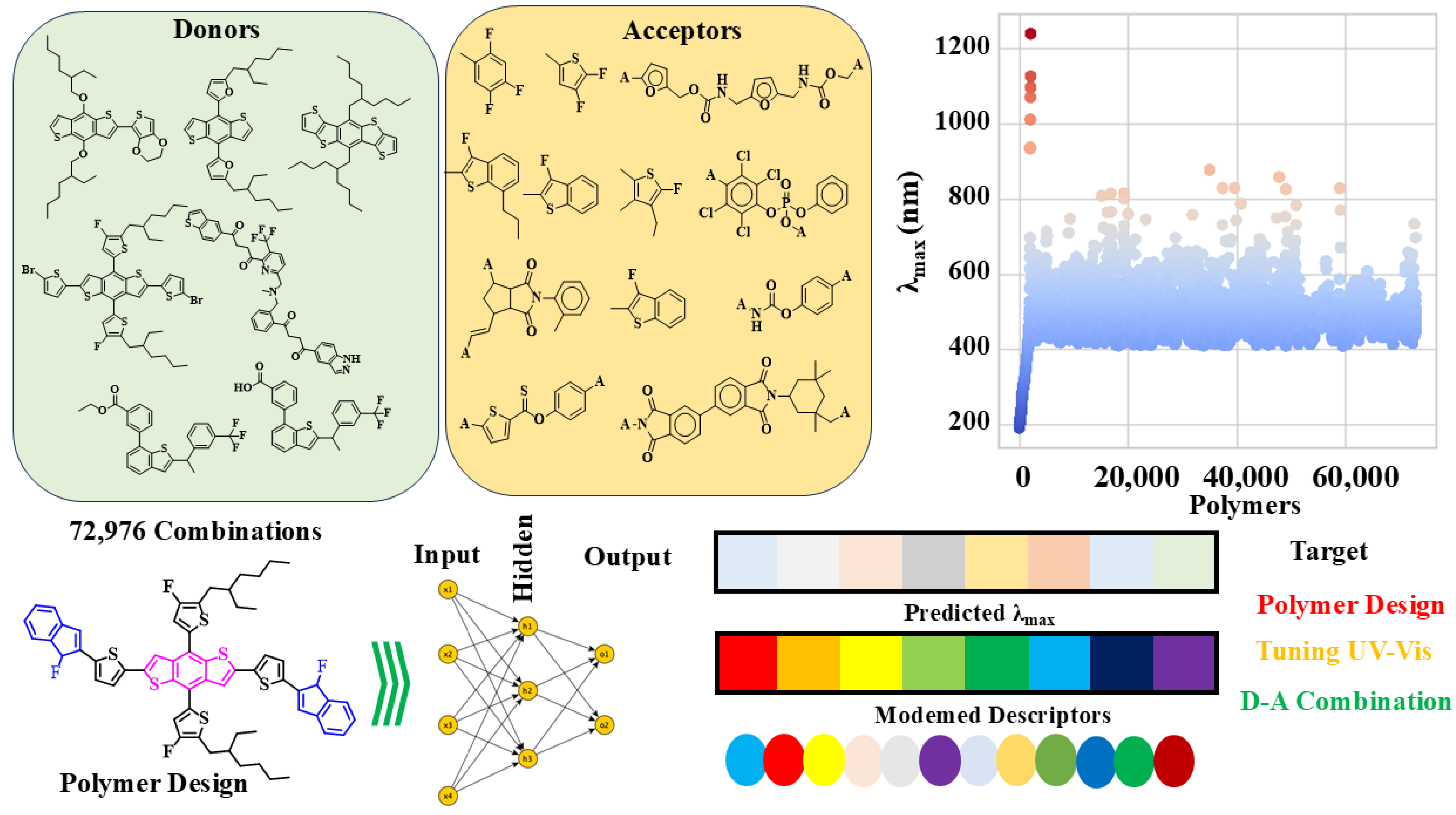
3.8. Throughput Screening for New Combinations

The collected data and trained model facilitated the design of 72,996 new combinations, each associated with their respective λ_max. This achievement was significant, as it enabled the exploration of a vast chemical space and the identification of novel compounds with favorable properties. The new combinations were generated by combining different molecular structures and functional groups, considering both the principles of chemistry and the limitations of the experimental design. The resulting compounds exhibited considerable diversity, encompassing a wide range of chemical properties, such as logP, molecular weight, and topological polar surface area. This diversity was crucial for investigating the structure–activity relationships and identifying the key factors that drive the λ_max of the compounds (Figure 8).

Different descriptors were developed for new combinations to aid in the accessibility studies. These descriptors included molecular fingerprints, such as MACCS and ECFP, which represented the structural characteristics of the compounds. In addition, physicochemical properties, including logP, molecular weight, and topological polar surface area, were computed for each compound. These descriptors were subsequently employed to analyze the correlations between the chemical structures and their λ_max. The design of the descriptors played a crucial role in the success of the accessibility studies. By integrating molecular fingerprints and physicochemical properties, the researchers were able to successfully capture the fundamental chemical and physical factors that influence the λ_max of the compounds. This approach facilitated the identification of key structural features and functional groups responsible for the λ_max, offering valuable insights into the underlying mechanisms that govern the absorption process. Furthermore, the descriptors were utilized to develop ML models capable of predicting the λ_max of new compounds. This enabled the rapid screening of extensive compound libraries, facilitating the identification of those likely to exhibit desirable absorption properties. The ML models were trained on an extensive dataset of experimental λ_max and validated with a selected subset of the data.

3.9. Computational Studies

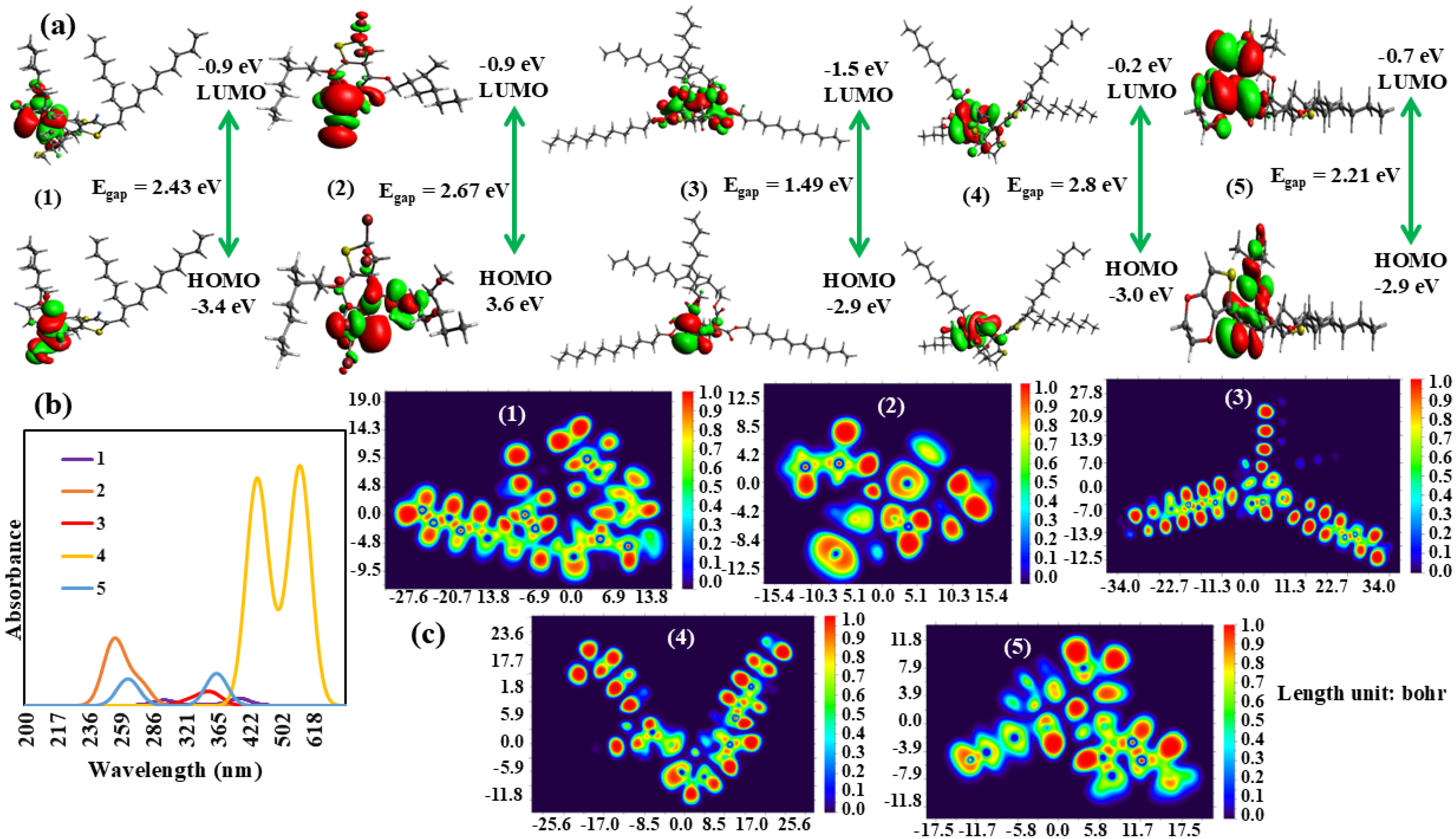
A computational study of selected polymers, utilizing the Density Functional Theory (DFT), was successfully validated to provide insights into their electronic properties. Their molecular geometries were optimized to their ground state energy minima using the CAM-B3LYP functional with the 6-31+G(d,p) basis set. Additionally, the computed TD-DFT spectra were obtained at the same level as the theory and basis set. Notably, the analysis revealed that the charges on the highest occupied molecular orbital (HOMO) and lowest unoccupied molecular orbital (LUMO) were primarily localized within the donor regions, exhibiting opposite charges [34]. This intriguing phenomenon suggested that the donor regions were crucial in governing the electronic behavior of polymers. In sharp contrast, the alkyl chains incorporated into these polymers were found to lack significant charges, implying that they do not substantially influence the electronic properties of the materials. These computational findings offered valuable insights for the design and development of novel polymers with tailored electronic properties, laying the foundation for potential applications in emerging fields such as optoelectronics and organic electronics. The computed UV-Vis parameters for the five polymers revealed distinct features. Polymer 1, exhibiting an energy of 3.10 eV and a wavelength of 401 nm, displayed a comparatively low oscillator strength (f) of 0.0012, reflecting a moderate absorption intensity (Figure 9). The predominant contribution to this polymer arose from the HOMO→LUMO transition, which accounted for the entirety (100%) of the transition. In contrast, polymer 2 exhibited a higher energy of 4.89 eV and a shorter wavelength of 257 nm, accompanied by a slightly increased oscillator strength (f) of 0.0016. The primary contribution to this polymer originated from the HOMO − 1→LUMO + 1 transition, which was responsible for 70% of the overall transition (

Table 3. Computed UV-Vis spectral analysis of the designed polymers.

Polymer	State	E (eV)	λmax (nm)	f	Major Contribs (%)
1	S0→S1	3.10	401	0.0012	HOMO→LUMO (100)
2	S1→S2	4.89	257	0.0016	HOMO − 1→LUMO + 1 (70)
3	S0→S1	3.46	358	0.0014	HOMO→LUMO (94)
4	S0→S1	2.21	563	0.0414	HOMO→LUMO (81)
5	S0→S1	3.43	363	0.0055	HOMO→LUMO (99)

). Polymers 3 and 5 displayed similar characteristics, exhibiting energies of 3.46 and 3.43 eV, along with wavelengths of 358 and 363 nm, respectively. Both polymers displayed relatively low f of 0.0014 and 0.0055, respectively, with the HOMO→LUMO transition being the dominant contributor, accounting for 94 and 99% of the transition, respectively.

Polymer 4 was characterized by a significantly lower energy of 2.21 eV and a longer wavelength of 563 nm, coupled with a relatively high f of 0.0414. The HOMO→LUMO transition was the predominant contributor to this polymer, responsible for 81% of the total transition. In addition to the electronic transitions, the electron localization functions (ELFs) [35] of these polymers yielded valuable insights into the spatial distribution of electrons. The red spots observed at the terminal regions of the polymers indicated regions of high electron density, which were likely engaged in electronic transitions. These regions may have been critical in determining the electronic and optical properties of polymers. For instance, in polymer 1, the ELF demonstrated a high electron density at the terminal regions, which corresponded to the HOMO→LUMO transition. This suggested that the electrons were localized in these regions, resulting in a moderate absorption intensity. In contrast, the ELF of polymer 2 exhibited a more dispersed electron density, which could be attributed to the involvement of HOMO − 1 and LUMO + 1 orbitals in the electronic transition. The similar electronic transitions observed in polymers 3 and 5 were also mirrored in their ELFs, which exhibited comparable electron density patterns.

The high electron density at the terminal regions in these polymers suggested a strong localization of electrons, which resulted in the observed low oscillator strengths. Polymer 4, characterized by its distinct electronic transition, displayed a more intricate ELF pattern featuring multiple regions of high electron density. This could be related to the longer wavelength and higher oscillator strength observed in this polymer.

The transition density matrix (TDM) analysis [36] provided comprehensive insights into the electronic transitions of the five polymers. The TDM plots, representing the probability density of the electronic transition, provided insights into the spatial distribution of the transition dipole moment. For polymer 1, the TDM plot exhibited a significant contribution from the ends of the polymer chain, signifying a strong dipole moment along the chain axis. This was consistent with the HOMO→LUMO transition, which predominantly governed this polymer. However, the TDM plot of polymer 2 exhibited a more intricate pattern, with contributions from both the terminal and the central regions of the chain, reflecting the involvement of HOMO − 1 and LUMO + 1. The TDM plots of polymers 3 and 5 showed comparable patterns, with predominant contributions originating from the ends of the chain, which corresponded to their HOMO→LUMO transitions. However, the TDM plot of polymer 4 displayed a unique pattern, with contributions from various regions along the chain, including both the ends and the middle, indicating a more delocalized transition dipole moment. This was consistent with the lower energy and longer wavelength observed in this polymer, which could be attributed to a more extended conjugation throughout the polymer chain. The TDM analysis also yielded insights regarding the directionality of the transition dipole moment, which could significantly impact the optical properties of the polymers. For instance, polymers 1 and 3 displayed a strong dipole moment along the chain axis, which might lead to a high absorption coefficient for light polarized in this direction. In contrast, polymer 4 exhibited a more isotropic transition dipole moment, which could lead to a lower absorption coefficient but may potentially enhance fluorescence efficiency.

The charge density difference (CDD) [37] analysis offered a comprehensive understanding of the electronic rearrangement that occurred during the electronic transitions of the five polymers. The CDD plots, which depicted the variation in electron density between the ground and excited states, revealed the areas of the polymer chain where electron transfer or redistribution took place during the transition. For polymer 1, the CDD plot indicated a notable transfer of electron density from the ends of the polymer chain towards the central region, which was consistent with the HOMO→LUMO transition. This suggested that the electrons were excited from HOMO to LUMO, leading to a redistribution of electron density along the chain. In contrast, the CDD plot of polymer 2 exhibited a more intricate pattern, showing both increases and decreases in electron density along the chain, which reflected the involvement of HOMO − 1 and LUMO + 1 orbitals. The CDD plots of polymers 3 and 5 exhibited comparable patterns, showing electron density transfer from the ends to the central region, which was consistent with their HOMO→LUMO transitions (Figure 10). However, the CDD plot of polymer 4 revealed a distinct pattern characterized by a substantial increase in electron density along the entire chain, suggesting electron delocalization during the transition. This showed consistency with the lower energy and longer wavelength of this polymer, which could be attributed to a more extended conjugation throughout the chain. Additionally, the CDD analysis revealed variations in electron density distribution between the ground and excited states, which could impact the optical properties of the polymers.

For instance, the CDD plot of polymer 1 revealed a notable increase in electron density near the ends of the chain, potentially leading to a higher absorption coefficient for light polarized in this direction. In comparison, the CDD plot of polymer 4 exhibited a more uniform increase in electron density across the chain, which might result in a lower absorption coefficient but could potentially improve fluorescence efficiency.

The global chemical reactivity parameters [38] of the five polymers offered crucial insights into their reactivity and chemical behavior. The ionization potential (IP) and electron affinity (EA) values demonstrated the energy required to remove or add an electron to the system, respectively. The electronegativity (χ) values, spanning from 1.63–2.28 eV, suggested that those polymers could exhibit moderate electronegativities, reflecting a balance between their electron-withdrawing and electron-donating abilities. The hardness (η) and softness (σ) values revealed information about the system with its resistance to electron transfer and its tendency to donate or accept electrons, respectively. The hardness values, ranging between 0.74–1.39 eV, suggested that these polymers exhibited moderate hardness, implying an intermediate resistance to electron transfer (

Table 4. Calculated global chemical reactivity parameters (eV) of selected polymers.

Polymer	IP	EA	χ	µ	η	σ	ω
1	3.43	1.00	2.21	−2.21	1.22	0.41	2.02
2	3.62	0.95	2.28	−2.28	1.34	0.37	1.95
3	2.97	1.49	2.23	−2.23	0.74	0.67	3.34
4	3.02	0.23	1.63	−1.63	1.39	0.36	0.95
5	2.92	0.70	1.81	−1.81	1.11	0.45	1.48

).

The σ values, spanning from 0.36–0.67 eV, revealed that these polymers exhibited moderate σ, suggesting their ability to moderately donate or accept electrons. The electrophilicity index (ω) values, varying from 0.95–3.34 eV, explained their ability to accept electrons and form bonds. The elevated electrophilicity index values suggested that some of these polymers exhibited a stronger inclination to form bonds and react with nucleophiles.

4. Conclusions

This study presents an advanced ML-assisted reverse polymer engineering approach to design high-performance benzothiophene/benzodithiophene polymers for photodetector applications. By harnessing the predictive capabilities of Gradient-Boosting Regression models, a comprehensive range of polymer combinations is swiftly screened to determine optimal structures with precisely tuned electronic properties. The success of this approach is highlighted by the achievement of exceptionally low bandgaps, reaching 0.42 eV, setting a new benchmark in the field of photodetector materials. The significance of this work stems from its potential to transform the discovery and design of high-performance polymers for advanced optoelectronic applications. The integration of ML algorithms with traditional materials design principles accelerates the discovery of innovative materials with superior properties, significantly reducing the time and cost required for experimental synthesis and characterization while unlocking new avenues for the development of high-performance photodetectors and other optoelectronic devices. Future research can focus on further enhancing the TAO approach to facilitate the design of polymers with more optimal properties and exploring its applicability to other classes of materials. Ultimately, this research can strive to establish ML-assisted reverse polymer engineering as a transformative strategy for developing high-performance materials with broad application potential.