Analysis of Corrosion Behavior and Cathodic Protection of Steel Pipeline Under Alternating Current Interference

Abstract

Alternating current (AC)-induced corrosion poses a significant threat to the integrity of underground pipelines, making it a critical concern for pipeline infrastructure. This study investigated the corrosion behavior of protected pipelines subjected to AC interference and developed practical tools to determine the required cathodic protection (CP) measures. Numerical models were developed to simulate current distributions in pipelines, incorporating the effects of metal types, CP levels, and varying AC interferences. These models were rigorously validated and calibrated using laboratory experiments to ensure their reliability. The models were then employed to analyze the corrosion behavior of pipeline metals under diverse CP and AC conditions. The results revealed the critical role of AC interference in aggravating corrosion rates and the diminishing effectiveness of CP at higher AC levels. Additionally, the study highlights the material-dependent nature of corrosion, with X60 pipe steel demonstrating superior resistance compared to C1018 pipe steel. Under the same AC and CP levels, the corrosion rate for C1018 pipe steel is 1.85 to 3.65 times higher than that for X60 pipe steel. Based on numerical analysis, empirical equations were developed to optimize the control of corrosion rates for both C1018 and X60 pipe steels under varying AC and CP conditions. The CP current density required to mitigate corrosion under an AC interference of 50 A/m² is 1.45 A/m² for C1018 pipe steel and 0.18 A/m² for X60 pipe steel. As AC interference increases to 500 A/m², the required CP current density rises to 2.98 A/m² for C1018 pipe steel and 2.2 A/m² for X60 pipe steel, highlighting the increasing demand for cathodic protection at higher AC levels.

1. Introduction

With the increase in energy demand and land use regulations, pipelines and high-voltage power transmission lines are frequently constructed to share the same route. The parallel power line orientations induce magnetic fields in the nearby pipelines, opposite to those in the power lines. The interaction between power lines and buried pipelines can be likened to the operational dynamics of a transformer. The power line functions as the primary winding, generating a magnetic field, and the pipeline acts as the secondary winding. This field can induce the flow of high levels of alternating current (AC) in the pipeline [1,2,3]. Such stray current can accelerate the electrochemical corrosion rate of buried pipeline metals and lead to serious corrosion damage. It has been found that AC-induced corrosion affects the integrity of underground pipeline [4,5], which is increasingly observed on a global scale [6,7,8].

Cathodic protection (CP) prevents the pipeline metal from corroding making it the cathode of an electrochemical cell. A cathodic protection system can be classified as a voltage-controlled CP when the voltage between the anodes and the pipe is controlled and as a current-controlled CP when the current in between is controlled. The most widely used cathodic protection standard [9] gives a CP potential of −0.85 V vs. a copper/copper sulfate electrode (CSE) (equal to −0.775 V vs. a saturated calomel electrode (SCE)) to provide adequate protection for steel pipelines [9]. However, the presence of an AC can reduce the protection effectiveness by shifting the applied CP potential from the desired value; as a result, both steel corrosion and cathodic reduction in dissolved oxygen are accelerated [10]. Currently, many studies have investigated the AC corrosion of protected pipelines through laboratory experiments. The general finding is that in the presence of AC originating from a laboratory’s supply machine, the CP potential might be shifted positively or negatively, depending on the AC and CP levels [11]. However, in both cases the metal has the potential to be corroded [12,13]. Therefore, the traditional −0.85 V (CSE) criterion is not sufficient to provide full corrosion protection. To protect buried metal from AC interference, a more negative CP potential might be needed [13], which needs to be determined based on the corrosion behavior.

The analysis of the corrosion behavior of pipeline metal under various AC interferences can be time-consuming with traditional experiments, and some influencing factors like metal properties, soil humidity, soil resistivity, and so on are difficult to evaluate [2]. Moreover, internal corrosion also occurs and can be influenced by the contents transported within the pipeline, operational conditions, and the internal environment of the pipeline. Each of these factors contributes to the overall corrosion mechanism and needs to be carefully analyzed to understand the degradation processes fully. Numerical simulation provides a solution to cost-effectively analyze the AC corrosion behavior under various conditions. Several numerical methods can be used to simulate the real system, including the boundary element method (BEM), the finite difference method (FDM), and the finite element method (FEM). Among them, the FEM is more suitable for corrosion modeling in millimeter-scale solutions, irregular meshing, and spatially varying reaction kinetics [14]. Current studies employing FEMs for AC corrosion analysis have investigated various scenarios, including pipeline metal with coating defects being subjected to AC while no CP is applied [15,16], a metal without coating under CP being subjected to AC [2,17,18], and metal being subjected to AC without a coating or CP [19].

For example, Ouadah et al. (2017) established an FEM model in which the sacrificial anode CP method was applied to the metal without a coating [2]. The results showed that the increase in the AC density caused a positive shift in the DC potential and an increase in the DC density, meaning corrosion would occur under AC interference and chemical reactions would happen on the metal surface. Wang et al. (2017) also developed an FEM model to investigate the impact of AC on the corrosion of a pipeline with coating defects [15]. The DC density at the edge of the defect was found to be obviously higher than that at the center of the defect, and the coated pipeline steel with smaller defects suffered more serious corrosion under the same level of AC interference. In addition, Cui et al. (2016) developed an FEM model to investigate the corrosion potential of an unprotected and uncoated pipeline which intersected with a protected one [19]. The results showed that the intersection area of the unprotected and uncoated pipeline has great potential to be corroded because of its higher DC density. Recently, Zhang et al. (2023) developed an FEM model to investigate the impact of an AC transmission line on pipeline cathodic protection [20]. It was found that AC transmission lines cause serious electromagnetic interference with the pipeline CP system, which will cause the CP potential to shift out of the effective protection area.

Previous studies have shown that numerical simulation is an effective tool for analyzing AC corrosion behavior. However, most of them focused on analyzing the impact of AC without exploring adjustments in CP measures in order to mitigate AC-induced corrosion. By quantitatively modeling corrosion behavior at various AC levels, the required CP measures considering AC’s impact can be determined [21]. Furthermore, most existing numerical simulations were conducted without experimental validation, which raises concerns about their accuracy and reliability in representing real-world corrosion behavior. Proper validation of the numerical model is essential to ensure reliability in assessing corrosion behavior under different AC and CP conditions, thereby enabling the accurate determination of the CP levels required to mitigate AC-induced corrosion. The objective of this study is to investigate the corrosion behavior of a cathodically protected pipeline under AC interference and propose CP measures required to mitigate AC corrosion. To achieve this objective, laboratory experiments that incorporate the effects of AC interference and cathodic protection were first conducted. Subsequently, numerical models were developed to simulate laboratory experiments and validated with experimental measurements. Finally, the numerical models were further used to analyze the corrosion behavior of metal under various AC and CP conditions, and the results were used to develop predictive equations to provide insights into adjustments in current CP measures. The novelty of this study lies in its integrated approach of combining numerical modeling with experimental validation and the establishment of empirical equations that enable adjustments in cathodic protection strategies, enhancing the effectiveness of infrastructure protection under variable environmental conditions.

2. Materials and Methods

Laboratory experiments were conducted to measure the corrosion rates of metal coupons under varying AC and CP conditions. Two types of metal were utilized: cold-finished 1018 (C1018) and API 5L X60 pipe steels, which were purchased from McMaster Carr (Elmhurst, IL, USA) and Metal Sample Company (Munford, AL, USA), respectively. It should be noted that C1018 steel was adopted as a substitute for API 5L X52 pipe steel due to its similar low-carbon composition and comparable yield strength, considering that X52 pipe steel was not readily available in this study. The chemical compositions of these two metals are presented in

Table 1. Metal coupon information.

Specimens	C (wt.%)	Mn (wt.%)	Si (wt.%)	P (wt.%)	S (wt.%)	Fe (wt.%)	Yield Strength (psi)
C1018	0.16	0.64	0.20	0.04	0.5	Bal.	54,000
X60	0.12	1.23	0.23	0.008	0.01	Bal.	60,000

.

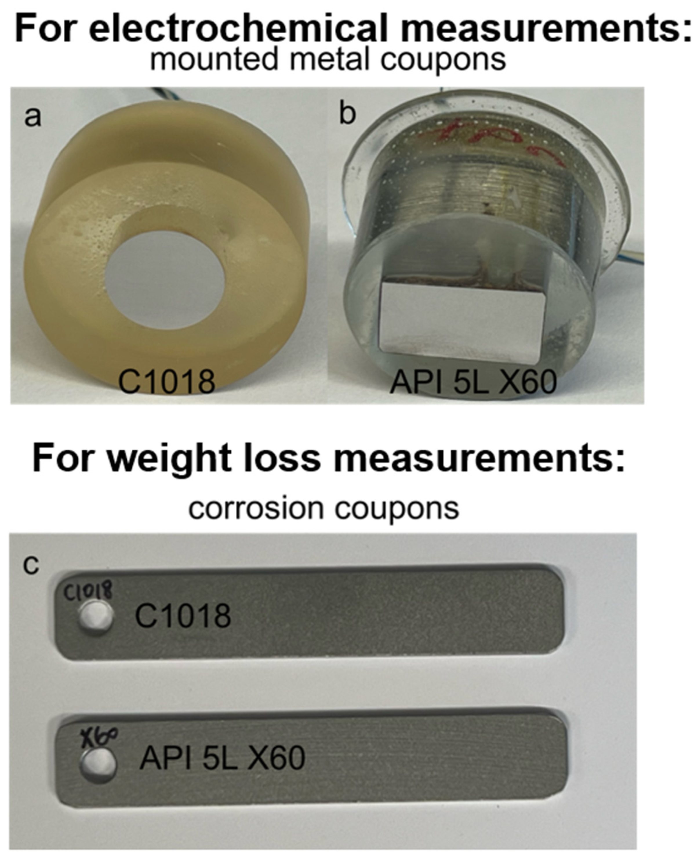
Two different types of coupons (mounted metal coupons and corrosion coupons) were used, as shown in Figure 1. The mounted metal coupons, as shown in Figure 1a,b, were used for electrochemical measurements. A copper wire was welded to the back of each cut metal sample to serve as the working electrode. Subsequently, the metals were meticulously sealed with epoxy, ensuring the absence of grooves or bubbles at the epoxy/steel interface. To achieve a smooth and uniform surface, the mounted steel surfaces were polished using 240-, 400-, 600-, 800-, and 1200-grit sandpapers, resulting in a mirror-like finish free from scratches. Then, the working area of each specimen was maintained at 2 cm² with Gamry PortHole Electroplating Tape. The corrosion coupons, shown in Figure 1c, were used for weight loss measurements. The mass loss was further used to indicate the corrosion rate. The corrosion coupons had dimensions of 7.6 cm × 1.3 cm × 0.16 cm. Prior to testing, the specimens underwent a thorough cleaning process using distilled water and acetone to ensure their cleanliness.

The test solution used in this study was a simulated soil solution consisting of 8.933 g/L KCl, 1.170 g/L MgSO₄·7H₂O, and 5.510 g/L NaHCO₃, with a pH of 8.08. This solution was designed to consider the major elements in soils according to a previous study [22]. The electric conductivity of the testing solution was 20 mS/cm, which was measured using the VWR 23226-505 Traceable Digital Conductivity Salinity TDS PPM Temperature Meter (from Avantor company at Radnor, PA, USA) in the laboratory. All solutions were prepared from analytical grade reagents and deionized water. All tests were conducted at room temperature (~22 °C) and exposed to air.

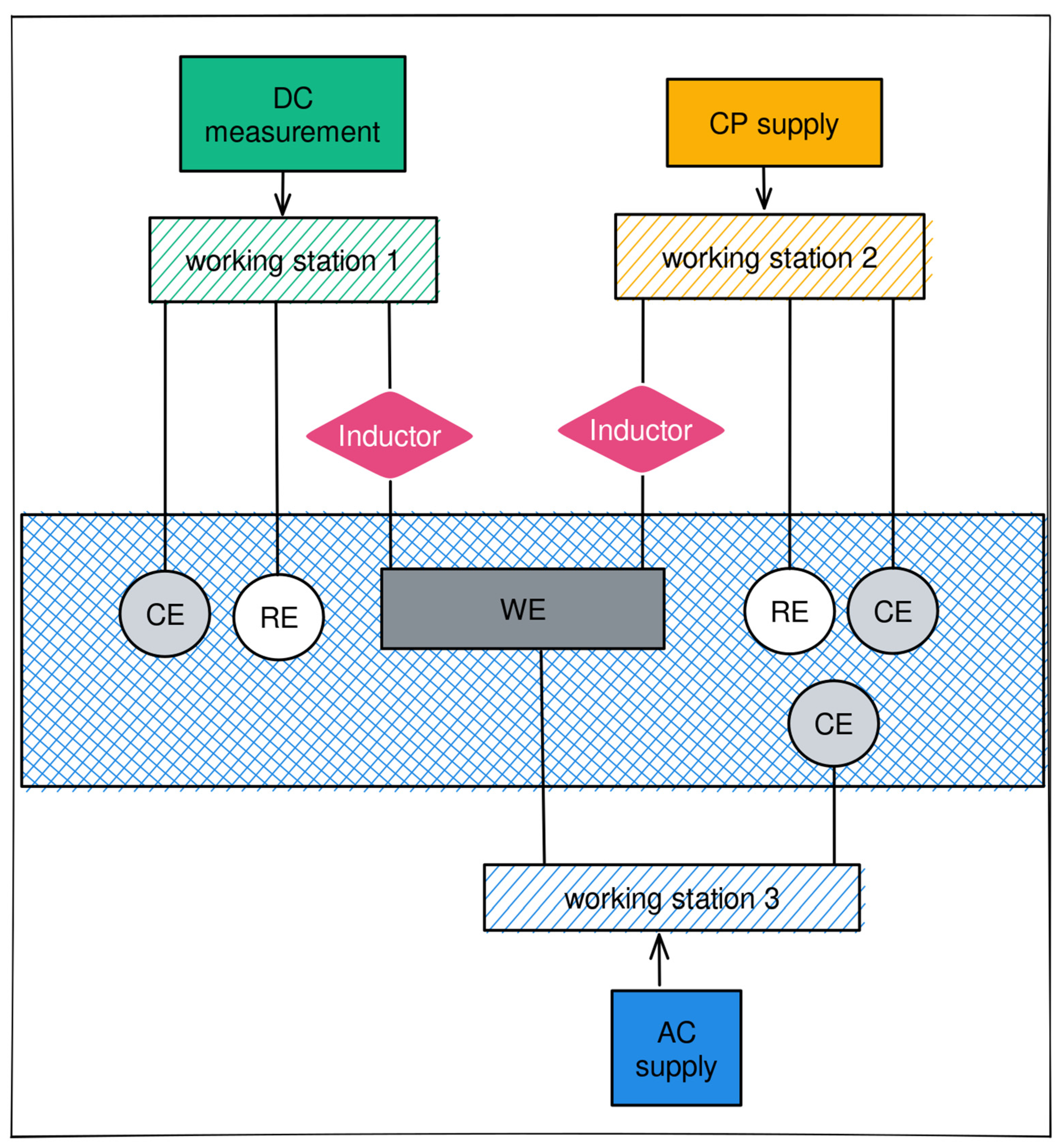
A schematic diagram of the electrochemical measurement and weight loss measurement of the pipe steel under various AC and CP conditions is shown in Figure 2. The DC circuit was executed by the Reference 600+ working station (from Gamry company at Warminster, PA, USA) (working station 1) with a three-electrode system consisting of a mounted metal coupon as the working electrode (WE), a saturated calomel as the reference electrode (RE), and a platinum sheet as a counter electrode (CE). In the AC circuit, a constant sine-wave AC with a frequency of 60 Hz was applied via the Virtual Front Panel (VFP) from another Gamry Reference 600+ working station (working station 2). The inductor element (10 Henries) was designed to prevent the AC from being released into working station 1. Also, working station 2 has built-in capacitor components to block the DC signals. The galvanostat applies a fixed CP current density on the working electrode, with DC potential as a response.

The corrosion coupons were cleaned according to the ASTM G1 standard and weighed before the test [23]. After the experiments, the corrosion product formed on the surface of the coupons was carefully removed using mechanical and chemical methods. Mechanical methods, including light scraping and scrubbing, were used to remove tightly adherent corrosion products. The chemical cleaning procedure followed ASTM G1 and was repeated several times to remove the corrosion product thoroughly. The cleaning process will not affect the mass loss measurement as it selectively targets only the corrosion deposits without removing any underlying material, preserving the integrity of the metal for accurate assessment. The weight loss of the pipe steel coupon was weighted with a Mettler Toledo ML104 Analytical Balance with an accuracy of 0.1 mg. Each weighing test was repeated three times to obtain an average value. The weight loss of the pipe steel was used to calculate the corrosion rate based on Equation (1) [8]. At least three duplicated samples were tested to obtain an average value for analysis.

$$CR={\displaystyle \frac{3.45\times {10}^6\times (W_0-W) }{S·t·\rho }}$$

(1)

where $CR$ is corrosion rate, mpy (mils per year); W₀ is the weight of the specimen before the experiment, g; W is the weight of the specimen after the experiment with the removal of corrosion products, g; S is the exposed area, cm²; t is the corrosion time, h; and $\rho$ is the density of the specimen, g/cm³.

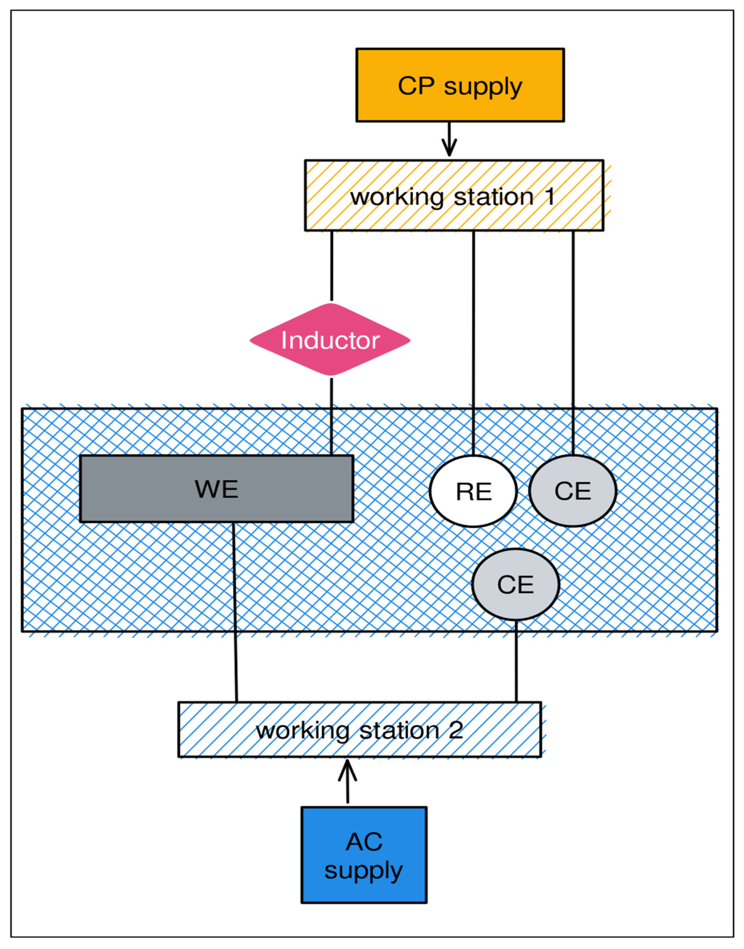
Figure 3 shows a schematic diagram of the potentiodynamic polarization measurement of the pipe steel under various AC and CP conditions. Potentiodynamic polarization is a technique that involves applying a voltage sweep to a metal and measuring the current feedback. The potential sweep ranged from −0.2 V to 0.2 V relative to the open circuit potential (OCP), with a scan rate of 0.2 mV/s. Before conducting the potential sweep, the OCP of the working electrode was measured for at least half an hour to ensure it reached a stationary value. Subsequently, the three-electrode system was used for the potentiodynamic polarization measurement. The potentiostat applies a constant CP potential to the working electrode, with a change in DC density as its feedback. The Tafel extrapolation method was used after the OCP to obtain the corrosion potential and corrosion current density. Finally, based on the parameters obtained from Tafel extrapolation, the corrosion rate was calculated using Equation (2). At least three duplicated samples were tested to obtain an average value for analysis.

$$CR={\displaystyle \frac{0.13\times i_{corr}\times M_w}{\rho }}$$

(2)

where $CR$ is corrosion rate, mpy (mils per year); $i_{corr}$ is corrosion current density, μA/cm²; $M_w$ is the equivalent weight of the corroding species, g; and $\rho$ is the density of the corroding species, g/cm³.

3. Development of AC Corrosion Model

3.1. Theory of Corrosion

The theory for the current distribution obeys Ohm’s law and the current conservation principle. Assuming electroneutrality (which cancels out the convection term), negligible concentration gradients of the current-carrying ion (which cancels out the diffusion term), and an approximately constant composition of charge carriers, the current density in the electrolyte can be written as Equations (3) and (4) [24], which can be further combined into Equation (5) in three-dimensional modeling.

$$i_k=-{\sigma }_k\nabla {\phi }_k$$

(3)

$$\nabla i_k={ Q}_k$$

(4)

$${\displaystyle \frac{{\partial }^2{\phi }_k}{\partial x^2}}+{\displaystyle \frac{{\partial }^2{\phi }_k}{\partial y^2}}+{\displaystyle \frac{{\partial }^2{\phi }_k}{\partial z^2}}={\displaystyle \frac{-Q_k}{{\sigma }_k}}$$

(5)

where Q_k denotes a general source term, k denotes an index that is l for the electrolyte and s for the electrode, ${\sigma }_k$ is the conductivity, and ${\phi }_k$ is the potential.

In the case of pipe corrosion, the pipe serves as the electrode and chemical reactions occur at both the anode and cathode under a typical alkaline environment that can be described in Equations (6)–(9). The primary anodic reaction in AC corrosion is the oxidation of the metal into metal ions. In the presence of AC, the cathodic reaction often involves the reduction of oxygen dissolved in the soil moisture. The interaction between the metal ions and the hydroxide ions can lead to the formation of various corrosion products. For example, the corrosion product magnetite (Fe₃O₄) may form a protective coating on the metal surface, while hematite (Fe₂O₃), which can also form, does not adhere well to metal and offers less corrosion resistance.

Anodic process:

Fe → Fe²⁺ + 2e⁻

(6)

Cathodic process:

4e⁻ + O₂ + 2H₂O → 4OH⁻

(7)

2e⁻ + 2H₂O → 2OH⁻ + H₂

(8)

2e⁻ + 2H⁺ → H₂

(9)

To characterize the electrochemical reactions that happened on the pipe steel, Tafel expressions were used to describe the electrode kinetics, as shown in Equations (10)–(12) [25]:

$$i_{c, local}=-i_{o,c}\times {10}^{{\displaystyle \frac{\mathsf{\eta }}{A_c}}}$$

(10)

$$i_{a, local}=-i_{o,a}\times {10}^{{\displaystyle \frac{\mathsf{\eta }}{A_a}}}$$

(11)

$$\eta ={ \Phi }_{\mathrm{s}}-{\Phi }_{\mathrm{l}}-E_{eq}$$

(12)

where i_c is the local current density at the cathode (A/m²); i_a is the local current density at the anode (A/m²); i₀ is the exchange current density (A/m²); η is the reaction overpotential; A_a and A_c are the Tafel slopes; ${\Phi }_{\mathrm{s}}$ is the electric potential; ${\Phi }_{\mathrm{l}}$ is the electrolyte potential (V); and E_eq is the equilibrium potential (V).

Since the anodic and cathodic chemical reactions occur simultaneously, the reaction rate can be calculated based on the local current density at either the anode or the cathode, as demonstrated in Equation (13). The corrosion rate of the metal can then be determined using Equation (14) [26]:

$$R={\displaystyle \frac{-v{i}_{local}}{nF}}$$

(13)

where R is the reaction rate (mol/(m²·s)); i_local is the local current density at the electrode (A/m²); n is the number of participating electrons; v is the stoichiometric coefficient for the reaction species (v = 1 for iron, v = −1 for oxygen, and v = 1 for hydrogen); and F is Faraday’s constant (F = 96,485 C/mol).

$$C_{rate}={\displaystyle \frac{MR}{\rho }}$$

(14)

where C_rate is the corrosion rate (mm/year); M is the molar mass of the anode (58 g/mol for iron); R is the reaction rate (mol/(m²·s)); and ρ is the density (7860 kg/m³ for iron).

3.2. Finite Element Model Development

The development of the numerical model includes several steps. Initially, the geometry of the model was created. Then, the governing equations of Ohm’s law and the current conservation principle were selected. Subsequently, the related chemical reactions were defined at the anode and cathode, respectively, and the boundary conditions on the electrodes were set. Material parameters were also assigned during this phase. Following the configuration of the meshing conditions, the stationary study was finally conducted.

A three-dimensional finite element model was created using COMSOL Multiphysics software (version 6.2) based on the laboratory testing conditions, as shown in Figure 4. The large cylinder represented the solution, and the small cuboid solid inside was the metal coupon, which was the cathode in this analysis. The diameter and height of the cylinder were 7 cm and 15 cm, respectively. The metal coupon was 7.6 cm long, 1.3 cm wide, and 0.16 cm thick. The diameter of the anode surface was 1 cm. The free tetrahedral mesh was applied to the model, and the mesh size of the extra fine mesh was selected in modeling based on the convergence analysis. There were a total of 328,381 elements.

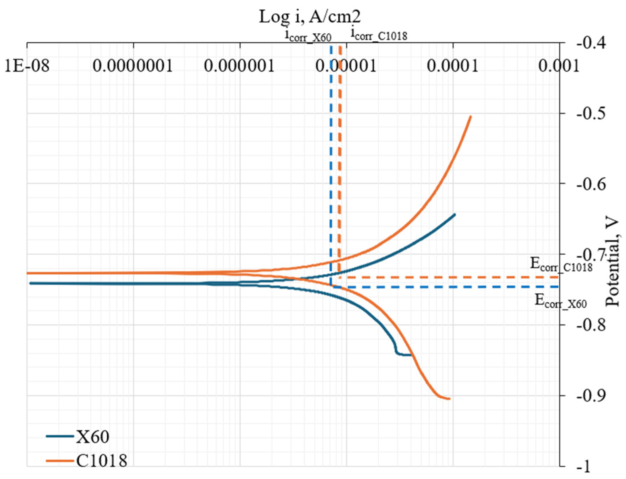
To characterize the electrochemical reactions on the metal surface, the polarization curves of the C1018 and X60 pipe steel were used as the boundary conditions for the cathode surface. This approach aligns with the methodology suggested in another simulation study conducted using COMSOL [27]. These polarization curves were obtained by instantaneously recording the direct current (DC) current density when changing the DC potential with a speed of 0.2 V/s in the laboratory experiments. An electric conductivity of 20 mS/cm was used for the solution, the same as was used in the laboratory experiment. The polarization curves in Figure 5 show that X60 pipe steel has a more negative corrosion potential than C1018 steel, indicating a greater thermodynamic tendency for corrosion. However, C1018 steel exhibits a higher corrosion current density, indicating a faster corrosion rate.

The reference electrode in this study was a saturated calomel electrode (SCE). The anode surface was set as an electrolyte potential surface with a potential value of 0 V vs. SCE. A CP current density was applied to the metal surface at −0.15 A/m², −0.4 A/m², and −0.75 A/m², respectively.

To account for the AC interference, an AC density which periodically reverses direction and changes its magnitude with time was applied to the pipe, as described in Equation (15) [18]. The magnitude of the AC density on the metal was selected as 0 A/m², 50 A/m², 100 A/m², and 200 A/m².

$$A_{\mathit{AC}}=\mathit{Asin}(2\pi \mathit{ft})$$

(15)

where A_AC is the AC density (A/m²); A is the magnitude of the AC current density (A/m²); f is the frequency, 60 Hz here; and t is the time (s).

3.3. Comparison Between Predicted and Measured Results

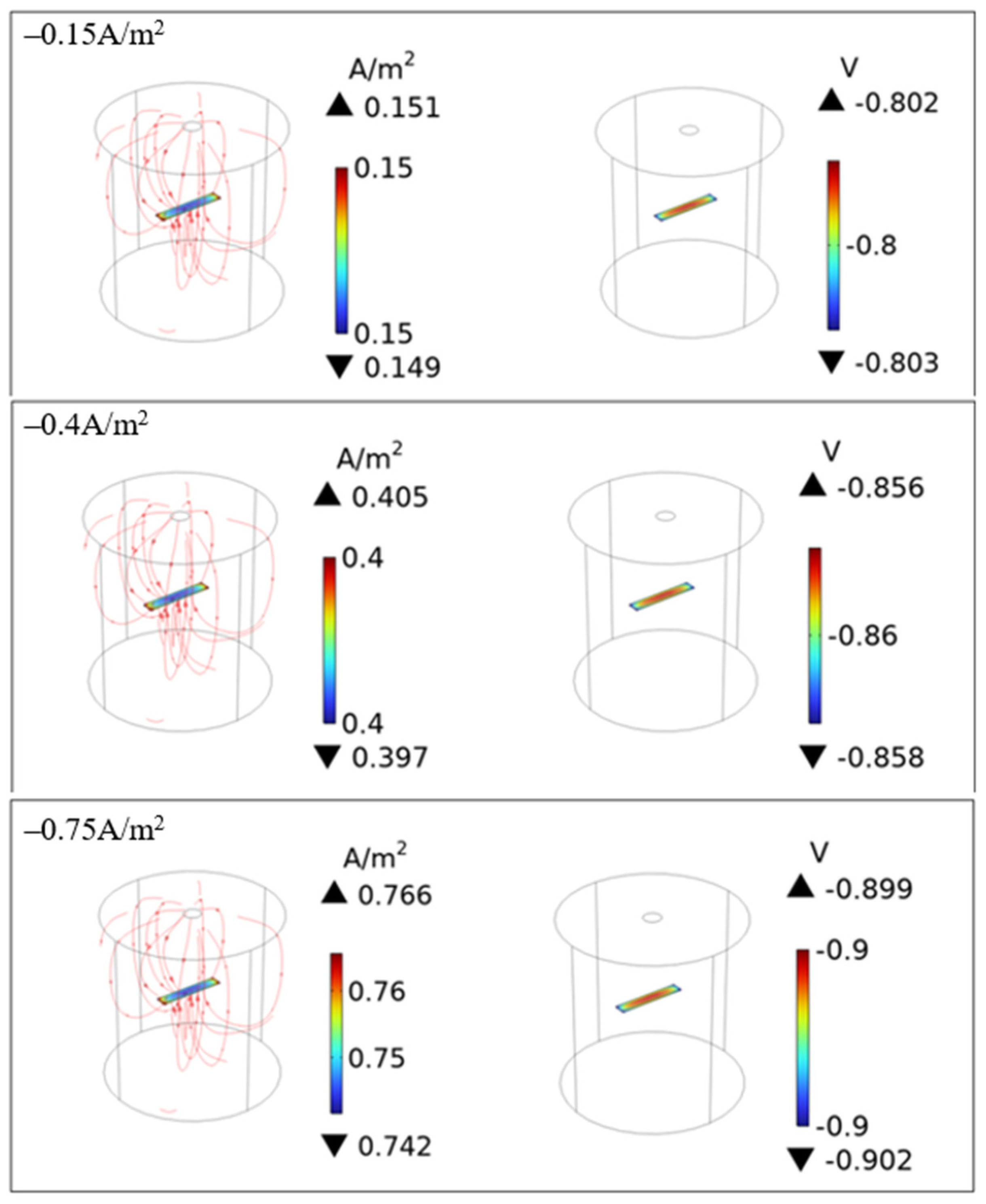
Figure 6 shows examples of the calculated DC density and potential on the surface of C1018 pipe steel after applying the CP current density without AC interference. As can be seen, when a −0.15 A/m² current density was applied, the DC potential on the metal surface was −0.8 V vs. SCE. As the CP current changed to −0.4 A/m² and −0.75 A/m², the DC potential further increased to −0.86 V and −0.9 V vs. SCE, respectively. These demonstrate a clear trend, where more negative CP current densities led to stronger protection, which is expected based on the current practice of impressed current cathodic protection (ICCP) for steel pipelines in the field.

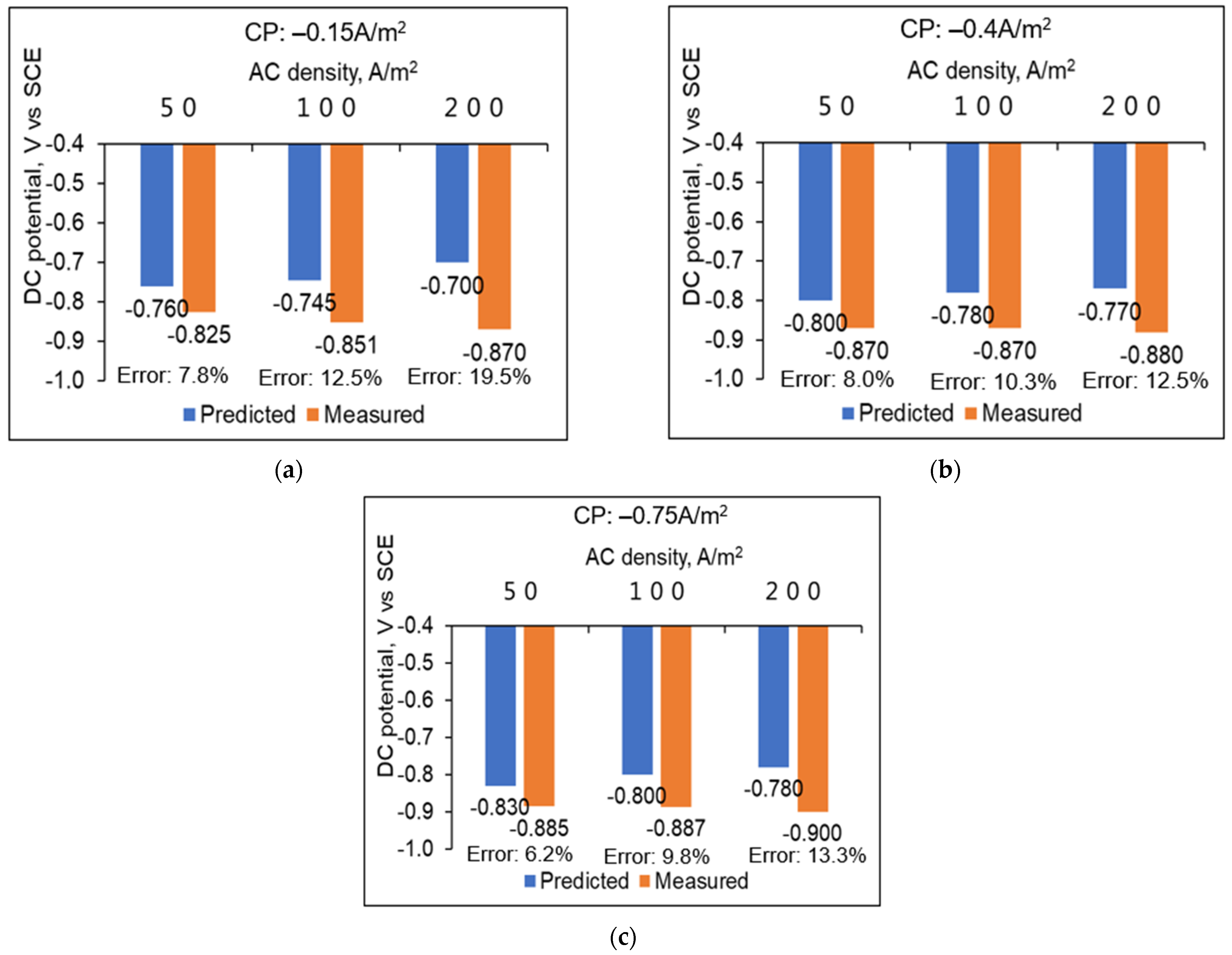
When applying a CP current density to achieve protection, comparisons between the predicted and measured DC potentials of C1018 pipe steel under AC interference are shown in Figure 7. This comparison revealed that the predicted values closely align with the measured potentials across various CP and AC densities, with errors less than 20%. Under the same AC density, both the predicted and measured DC potential shifted negatively as the CP current density became more negative. This means that, to mitigate AC corrosion, the CP current density can be increased to render the DC potential more negative. However, it should be cautiously calibrated to prevent over-polarization, and the specific environmental conditions and metal properties should be considered to balance corrosion protection with potential adverse effects. Under the same CP current density, the predicted DC potential shifted positively with the increase in AC density. However, contrary to expectations, the measured DC potential shifted negatively. This suggests that while an increase in AC density is theoretically expected to accelerate corrosion, an experimental protection effect was noted, contradicting with the engineering judgment that, with AC interference, the AC density will aggravate corrosion. This phenomenon was also observed in other studies [12,13], while the mechanism behind it is still inconclusive.

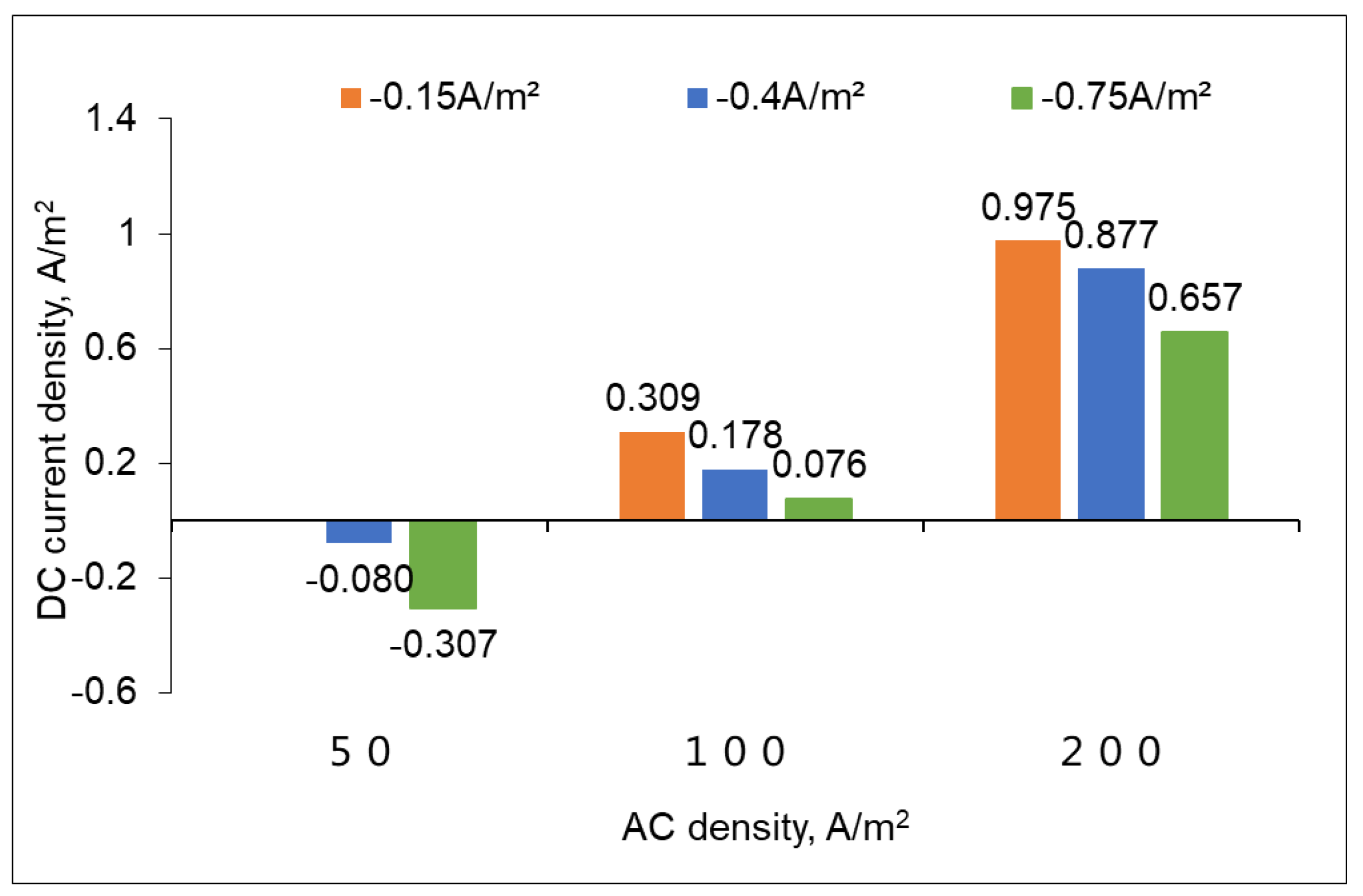
Considering that the DC densities could not be measured in the laboratory, Figure 8 shows the predicted DC densities of C1018 pipe steel under various AC interference levels. It can be seen that the DC density shows a remarkable difference under different CP and AC densities. The DC density shifted positively as the AC density increased or the CP current density became less negative. When the AC density was 100 A/m² or 200 A/m², the DC densities were positive under all CP levels. This means that the cathodic protection is no longer effective under this circumstance. It was reported that when the AC stray current density remains at or below 100 A/m², pipe steel corrosion predominantly manifests as uniform corrosion. As the AC stray current density increases beyond this level, the passivation film will be reduced, leading to localized anodic breakdown. This disruption promotes pit initiation, where chloride ion accumulation and acidification inside the pits accelerate localized metal dissolution, transitioning from uniform to pitting corrosion. Notably, at an AC stray current density of 200 A/m², there is a clear shift towards pronounced localized corrosion, which is pitting damage [28]. Therefore, a more negative CP current density is needed in order to protect the pipeline from AC corrosion.

In the laboratory, two distinct methods were employed to measure the corrosion rates of metal: the mass loss method and the Tafel method.

Table 2. Corrosion rates obtained from various methods.

AC, A/m2	CP, A/m2	C1018		X60
		Weight Loss, mm/y	Tafel Method, mm/y	Weight Loss, mm/y	Tafel Method, mm/y
50	−0.75	0.04	0.11	0.02	0.08
100	−0.75	0.16	0.18	0.05	0.12
200	−0.75	0.28	0.25	0.20	0.15
50	−0.4	0.06	0.14	0.05	0.09
100	−0.4	0.21	0.20	0.11	0.15
200	−0.4	0.35	0.30	0.30	0.18
50	−0.15	0.17	0.17	0.11	0.10
100	−0.15	0.24	0.24	0.19	0.16
200	−0.15	0.42	0.31	0.30	0.19
0	0	0.24	0.10	0.19	0.08
50	0	0.26	0.18	0.24	0.11
100	0	0.35	0.24	0.31	0.18
200	0	0.53	0.33	0.37	0.20
0	−0.75	0.07	0.07	0.04	0.04
0	−0.4	0.11	0.08	0.06	0.05
0	−0.15	0.21	0.08	0.11	0.05

summarizes the corrosion rate results under various conditions. It can be found that the corrosion rates calculated from two methods have certain differences. Thus, the average corrosion rates obtained from these two methods were used and compared here. Figure 9 presents the correlations between prediction and measurements for both C1018 and X60 pipe steels. The results indicate a strong correlation, with R-square values ranging from 0.85 to 0.91. This demonstrates that, despite minor discrepancies, the numerical model effectively captures the general trends of corrosion, which allows it to provide reliable analyses of AC corrosion behavior under various conditions.

4. Analysis of Corrosion Rate Under Various AC and CP Levels

4.1. Corrosion Rates Under Varying CP and AP Conditions

Figure 10a,b show the impact of CP and AC levels on the corrosion rate for C1018 and X60 pipe steel, respectively. The ICCP method was selected for analysis here because it is often used as the main method for regional cathodic protection in practice and has the characteristic of continuous corrosion prevention [28]. For both pipe steels, it was observed that an increase in AC density or a decrease in CP current density led to a corresponding rise in the corrosion rate. This trend highlights the detrimental effect of AC interference on the protective efficiency of the CP system. Notably, the rate of corrosion accelerated more significantly as the AC density increased, regardless of the CP current density. This indicates that higher levels of AC interference can greatly exacerbate the corrosion process. Conversely, as CP current density becomes more negative, the corrosion rate decreases due to increased electron supply, which inhibits anodic dissolution. However, the reduction in corrosion rate slows at higher CP levels, indicating diminishing protection efficiency. While increasing CP current enhances corrosion protection, excessive current can lead to overprotection effects such as hydrogen embrittlement or coating damage. Therefore, optimizing CP current density is crucial to achieving effective protection without unintended consequences.

When comparing the two materials, it is evident that the corrosion rate of X60 pipe steel was significantly lower than that of C1018 pipe steel under similar conditions. Under the same AC and CP levels, the corrosion rate of C1018 pipe steel is 1.85 to 3.65 times higher than that of X60 pipe steel. It means that the inherent properties of the material, such as its composition and microstructure, play a crucial role in its corrosion behavior.

4.2. Adjustment in CP Measures Considering AC Interference

To facilitate the analysis of AC-induced corrosion, the corroison rate was regressed using CP and AC densities based on the results shown in Figure 10. The regression equaitons were fitted and are shown in Equations (16) and (17) for C1018 and X60 pipe steels, respectively.

$$R_{C1018}=0.14\ast {{CP}_c}^2+0.36\ast {CP}_c+0.00000395\ast {{AC}_c}^2-0.000255\ast {AC}_c+0.3585$$

(16)

$$R_{X60}=0.14\ast {{CP}_c}^2+0.28\ast {CP}_c+0.00000216\ast {{AC}_c}^2-0.000241\ast {AC}_c+0.1752$$

(17)

where ${CP}_c$ is the applied CP current density, A/m², and ${AC}_c$ is the AC density A/m².

Table 3. Evaluation metrics of developed empirical models.

Metal	CP Measures	R2	MAE	p-Value
C1018	CP current density	0.99	0.023 mm/yr	1.00
X60	CP current density	0.98	0.017 mm/yr	0.98

presents the evaluation metrics for the developed empirical models. The results show that the corrosion rates calculated using the regression equations align closely with the original data, with R² values exceeding 0.95 for both C1018 and X60 pipe steels. Regarding the mean absolute error (MAE), when a CP current density was applied, the MAE was 0.023 mm/yr for C1018 pipe steel and 0.017 mm/yr for X60 pipe steel. When a CP potential was applied, the MAE values were slightly higher, at 0.07 mm/yr for C1018 pipe steel and 0.047 mm/yr for X60 pipe steel. These small error values demonstrate the high accuracy of the regression equations in reliably estimating corrosion rates under various CP and AC levels. To further validate the empirical models, a Student’s t-test was conducted to assess whether the corrosion rates derived from the regression equations significantly differed from the original data. The analysis produced p-values of 1.0 for C1018 pipe steel and 0.98 for X60 pipe steel when a CP current density was applied and 0.512 and 0.994 for C1018 and X60 pipe steels, respectively, when a CP potential was applied. These p-values indicate no statistically significant difference between the calculated corrosion rates and the original data at a 95% confidence level.

A corrosion rate of 0.1 mm/yr is recognized by the European standard as the “safe” threshold as it is sufficiently low so that during the design lifetime, corrosion damage cannot occur [29]. In addition, Ormellese et al. (2015) conducted laboratory experiments and specified that beyond this level, there is high corrosion risk and this cannot be negligible [30]. Therefore, the developed empirical model was applied to determine the required CP levels under varying AC conditions, using a corrosion rate of 0.1 mm/yr as the threshold, as shown in Figure 11. The results indicate that higher AC interference levels necessitate greater CP current density to protect pipeline metals from AC-induced corrosion. For example, to prevent AC corrosion at a moderate interference level of 50 A/m², 1.45 A/m² is needed to protect C1018 pipe steel, whereas 0.18 A/m² is sufficient for X60 pipe steel. Under a severe AC interference level of 500 A/m², the required CP current density increased to 2.98 A/m² and 2.2 A/m² for C1018 and X60 pipe steel, respectively. It is noted that these threshold values of CP current are developed for the steep coupon in laboratory conditions, and further work needs to be conducted for the site-specific CP system design to effectively mitigate the AC-induced corrosion of real pipelines in a soil environment.

5. Conclusions

This study aimed to develop and utilize numerical simulations to analyze AC corrosion behavior and determine the required cathodic protection measures. Numerical models were developed to simulate electrochemical processes and current distributions in pipelines exposed to AC interference. These models incorporate the effects of metal types, AC interferences, and cathodic protection levels. The numerical models were rigorously validated and calibrated against laboratory experiments, ensuring accuracy in predicting CP performance change and corrosion rates due to AC interference. Based on the results from this study, the following conclusions can be drawn.

• It was found that AC interference significantly exacerbates corrosion rates, diminishing the effectiveness of conventional CP measures.
• This detrimental impact varies depending on the pipeline steel used. Under identical AC and CP conditions, the corrosion rate for C1018 pipe steel is 1.85 to 3.65 times higher than that for X60 pipe steel, underscoring X60’s superior corrosion resistance.
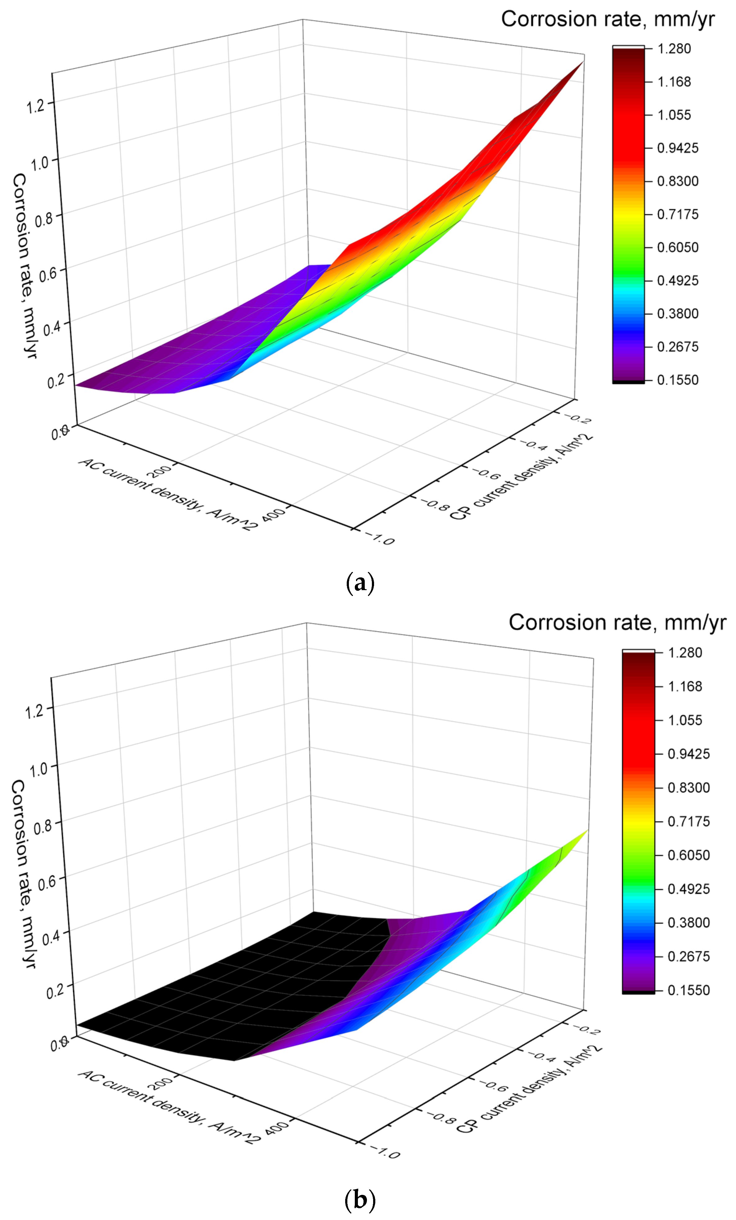
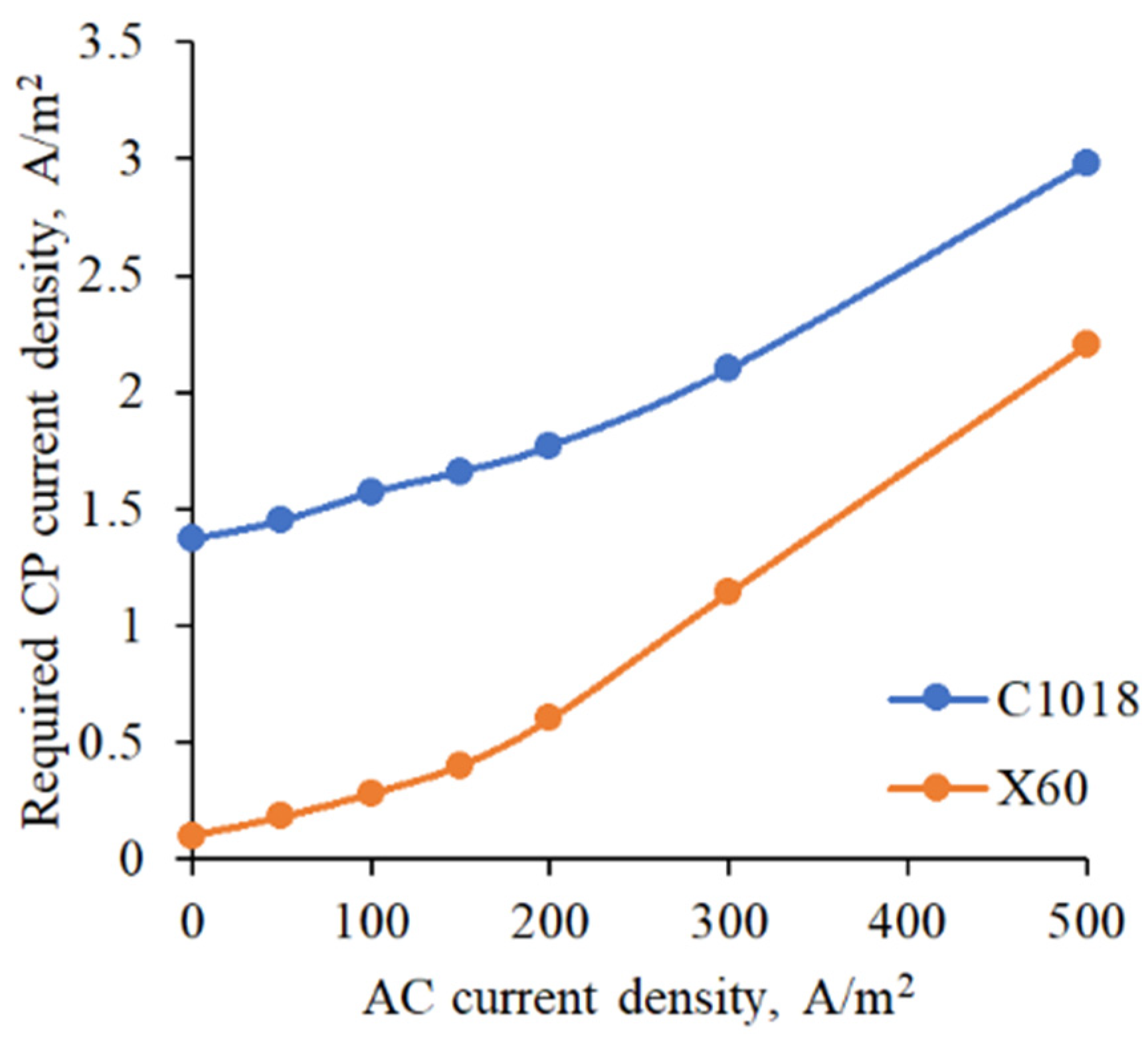
• Based on the simulation results, regression equations were established to estimate the corrosion rates of a pipe steel coupon under various CP and AC levels, which can be used to determine the CP levels required to mitigate the impact of AC.
• To prevent AC corrosion at a moderate interference level of 50 A/m², 1.45 A/m² is needed to protect C1018 pipe steel, whereas 0.18 A/m² is sufficient for X60 pipe steel. Under a severe AC interference level of 500 A/m², the required CP current density increased to 2.98 A/m² and 2.2 A/m² for C1018 and X60 pipe steels, respectively.

To enhance the applicability of the results, future research is recommended to expand the numerical models for real pipelines by incorporating additional factors such as soil properties, coating defects, and other environmental variables. This would enable a more comprehensive analysis of corrosion behavior under diverse real-world scenarios, providing broader insights for practical applications. In addition, it is recommended to investigate the transition from uniform to pitting corrosion under high AC interference levels, investigating the critical thresholds and electrochemical mechanisms that drive localized corrosion. This will enhance our understanding of AC corrosion and aid in developing more effective mitigation strategies.