A Model for Predicting 3D Wear Morphology of Ball-End Milling Tools: Development and Validation

Abstract

Tool wear prediction is an important research area in the machining industry, which can maximize the utilization of tools. Titanium aluminum alloy is the most commonly used material in the aerospace field, and it is difficult to process. Therefore, the tool wear in the machining process is serious and non-linear. This results in unpredictable tool wear. In this paper, a three-dimensional (3D) shape prediction method for milling wear of a ball-end milling cutter is proposed. By accurately predicting the tool wear volume, a customized tool dulling standard based on the tool damage percentage is established. Based on the tool material wear rate model and discrete analysis, the force, cutting temperature, relative contact time, and sliding speed of each element in the cutting process of the ball-end mill are solved. Combining the analysis results with the wear rate model, the original model of tool 3D wear morphology (3DWM) prediction was established. Finally, the experiment of cutting titanium aluminum alloy with a carbide tool is carried out to verify the proposed method. The results show that the approximate degree of the wear shape predicted by the model is up to 83.2%.

1. Introduction

Titanium aluminum alloy is commonly used in aerospace manufacturing. This is due to its low weight and high strength. The result of high strength is serious tool wear during machining. The occurrence of tool wear will not only affect the surface integrity of the workpiece [1] and reduce the quality of the workpiece but also lead to decreased production efficiency and shorter tool life. The aerospace field has high precision requirements for the workpiece. Therefore, the tool wear is studied to predict the tool wear morphology. It is of practical significance to improve machining quality and tool life by adjusting machining parameters according to wear morphology and reducing the influence of wear on machining quality. At present, the research of cutting tool wear can be divided into the research of cutting tool wear mechanism and the use of big data for real-time monitoring and prediction of cutting tool wear. The mechanism of cutting tool wear is an important part of cutting tool wear research. In this regard, H. Takeyama et al. [2] conducted basic research on cutting tool wear and tool life from the angle of tool edge wear. X Luo et al. [3] used a new model combining cutting mechanics simulation and empirical function to predict the wear rate of the flank face of cemented carbide blade in the metal cutting process. Yung-Chang Yen et al. [4] discussed a numerical implementation method combining the cutting tool wear model with finite element calculation to predict the evolution of cutting tool wear during long cutting cycles. Ryosuke Kataoka et al. [5] proposed and verified a new hypothesis in order to better understand the relationship between the evolution of tool face wear and its mechanism, that is, the tool face wear part keeps the geometric shape similar in the steady-state wear region while still expanding. Arsecularatne JA et al. [6] studied the wear mechanism of cutting tools made of tungsten carbide (WC), PCBN, and PCD by using the tool life and temperature results in the literature. M. Ben Said et al. [7] proposed an analytical model to estimate the relationship between cutting force, tool geometry, chip geometry, and flank face wear during milling with a ball-end mill. De Jun Cheng et al. [8] proposed a time-varying surface roughness model considering the overlap distribution of cutter teeth wear for multi-axis ball-end milling cutters, taking into account the tool geometry, single-tooth wear overlap distribution, tool runout, and wear overlap region. Nouni Mehdi et al. [9] propose a new method for real-time monitoring of end mill cutting tool wear by tracking the force model coefficient during the cutting process. This method can be used to track cutting tool wear in real time and detect the transition point from the gradual wear area to the failure area where the wear rate accelerates. Fernando Ramirez P. et al. [10] proposed and demonstrated a general method based on dimensional analysis and finite element analysis. This method is used to simulate the progress of pitting wear on cutting tools in steel processing. Ma Lianjie et al. [11] proposed the furring effect wear mechanism of cutting tool wear of turning brittle materials and established the friction coefficient model between the tool tip wear surface and the workpiece surface on the basis of tribological principles and the turning test of fluoroglyphite glass-ceramics. Zhuang Kejia et al. [12] developed an analytical model based on the slip line theory and extracted an imaginary heat source formula for a wear tool with cutting edge geometry from the steady wear stage. These formulas relate the phase of steady wear to the phase of sharp wear. However, the wear model mentioned above is not suitable for intermittent machining. For this reason, Chengdong Wang et al. [13] established a mathematical model of cutter face wear by obtaining cutting force and cutting temperature in real time. Chuandong Zhang et al. [14] propose a cutting tool wear prediction method based on the symmetric lattice and multi-covariance Gaussian process regression.

However, for different tools and workpiece materials, the rule of cutting tool wear will be different. Lin Zhou et al. [15] proposed a semi-analytical model considering the change in cutting edge wear and the related non-linear process characteristics for the estimation of cutting force during the milling of NAK80 steel micro ball head. Deng Jianxin et al. [16] carried out dry cutting experiments on Ti-6Al-4V alloy with WC/Co cemented carbide cutting tools to study the diffusion of elements from Ti-6Al-4V titanium alloy to WC/Co cemented carbide cutting tools at temperatures up to 800 °C. S Wojciechowski et al. [17] evaluated the ploughing phenomenon by studying the ploughing force at the tool flank face–workpiece interface during the milling process of AISI L6 alloy steel precision ball-end. Yu Liu et al. [18] studied the effects of different amounts of WC-TiC ceramic particles on the friction and wear properties of Ni-based alloy coatings. Junhua Liang et al. [19,20] studied the cutting tool wear microstructure, cutting tool wear curve, tool cutting force, and cutting tool wear mechanism of coated cemented carbide tools in the process of GH4169 dry-cutting. In addition to material, cooling conditions also have an impact on cutting tool wear. Munish Kumar Gupta et al. [21] found that under the condition of liquid nitrogen cooling and lubrication, the workpiece obtained smooth surface quality compared with dry conditions, which minimized the accumulated edge of the chip and reduced cutting tool wear. Jay Airao et al. [22] combined liquid CO₂ minimal quantity lubrication with ultrasonic vibration-assisted machining to analyze cutting tool wear patterns and behaviors under different cooling strategies. These studies and experiments have studied the mechanism of cutting tool wear from different angles, but they have not been able to predict the 3D morphology of cutting tool wear.

With the rise of big data network modeling technology, this technology is also used by researchers in the field of cutting tool wear research. Chen Zhang et al. [23] proposed a new online measurement algorithm for cutting tool wear, which used machine vision to obtain cutting tool wear, establish an online monitoring model for cutting tool wear, and evaluate the wear degree and remaining service life of the tool. Minghui Cheng et al. [24] proposed a comprehensive cutting tool wear monitoring model based on feature normalization, attention mechanism, and hierarchical parallel CNN. Then, a cutting tool wear prediction model based on a dense residual neural network is proposed to realize the multi-step prediction of the cutting tool wear value in the near future. Yuqing Zhou et al. [25] proposed a new and improved multi-scale edge-marked graph neural network to improve the recognition accuracy of cutting tool wear monitoring based on deep learning under small samples. However, in the process of cutting tool wear image acquisition, there are problems such as loud noise, blurred boundaries, and misalignment. To solve these problems, Kunpeng Zhu et al. [26] proposed a region growth algorithm based on morphological component analysis (MCA), and based on this algorithm, proposed a cutting tool wear surface area monitoring method based on the whole cutting tool wear image. Zhiwen Huang et al. [27] proposed a cutting tool wear prediction method based on multi-domain feature fusion of deep convolutional neural network (DCNN). This method extracts multi-domain (time domain, frequency domain, and time-frequency domain) features from 3D multi-sensory signals such as cutting force and vibration as health indicators of cutting tool wear, then directly establishes the relationship between these features and real-time cutting tool wear based on the designed DCNN model, and combines adaptive feature fusion with automatic continuous prediction to improve the cutting tool wear prediction accuracy. Qinglong An et al. [28] introduced a hybrid model, CNN-SBULSTM, which combines convolutional neural network (CNN) with bidirectional and unidirectional stacked LSTM (SBULSTM) networks to realize cutting tool wear evolution tracking and tool remaining service life prediction. Rongyi Li et al. [29] established a channel spatial attention mechanism to evaluate the effectiveness of different cutting tool wear signal features. These big data algorithms can use different signal inputs to identify or predict the average wear value or wear state of the tool. However, these studies have not been able to predict the amount of wear at any specific point on the tool.

Although these experiments and studies reflect the causes of cutting tool wear to a certain extent, they also successfully predict the wear amount or wear width of cutting tool wear. However, only the two-dimensional wear amount of the cutting tool is predicted, while the 3DWM analysis is ignored. This oversight can lead to inadequate real-time control of the cutting tool’s wear shape during the machining process, resulting in misjudgment of the tool’s wear state. Consequently, this affects the adjustment of machining parameters during the process. The tool wear is very time-varying and affected by many factors, so it is difficult to accurately predict the 3DWM. Therefore, there are still a few studies on 3DWM prediction. These studies have not been able to predict the amount of wear at any specific point on the tool. The 3DWM of the tool is not predicted. In order to solve the above problems and fill the gap in the research field, this paper focuses on the prediction of 3D cutting tool wear morphology. Therefore, this paper attempts to predict the wear shape of a ball-end milling cutter by using the micro-element method combined with the wear rate model of cutting tool wear, innovatively proposes a tool section wear shape prediction method based on material removal, and carries out theoretical analysis and experimental verification. The main expected contributions of this paper are as follows:

(1)

In this paper, the micro-element method is applied to the study of cutting tool wear morphology prediction. The effective contact region in the tool is divided into several iterated point elements. Based on this, the wear amount of any point on the tool is predicted by the wear rate model.

(2)

Based on the wear rate model, this paper analyzes the forces at any point of the tool, the tool–workpiece transient cutting contact relationship, and the temperature of the tool during the machining process. The accuracy and reliability of cutting tool wear prediction at any point are improved by combining these three parameters.

(3)

Combining the wear rate model with wear morphology prediction, a 3D cutting tool wear morphology prediction method based on material removal was proposed. This method can superimpose the wear amount of each iteration point on the milling cutter through iterative calculation and show the evolution process of cutting tool wear. The reliability of the method is verified by experiments.

2. Tool Wear Morphology Prediction Model of Ball-End Milling

2.1. Wear Rate Model

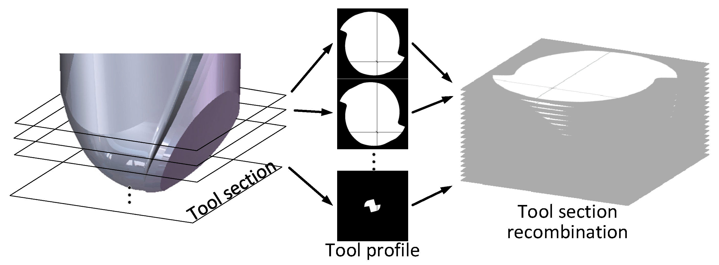
Before the research on the cutting tool wear morphology prediction method, in order to eliminate special cases and improve the accuracy of the method, the following assumptions were made about the cutting system: (1) the milling process is stable, and no flutter occurs; (2) there is no reinforced edge on the milling cutter; (3) there is no difference in the wear of each tool tooth. On the basis of this, the paper assumes that the surface material of the tool will form a flake every time the tool is impacted, and the blade is divided into several micro units for the iterative calculation of the material flake.

In this paper, the ball-end milling cutter is divided into several sections, and the section shape of the unworn tool section is obtained. Then the tool cross-section after wear is calculated according to the wear rate model, and the cross-section is reorganized to obtain the 3DWM, as shown in Figure 1. In general, cutting tool wear is mainly due to the cutting and extrusion of the blade on the workpiece material during the machining process, the force of the workpiece material on the rake face, and the friction between the flank face and the machined surface. The cutting tool wear rate model is shown as follows:

$${\displaystyle \frac{dw}{dt}}={\displaystyle \frac{A}{H}}{F}_n{V}_s+Bexp\left({\displaystyle \frac{-E}{R{T}_f}}\right),$$

(1)

where $w$ is the volume of cutting tool wear, $A$ is the abrasive wear constant, $H$ is the hardness of the tool material, $V_s$ is the sliding speed between the tool surface and the workpiece, ${\sigma }_n$ is the normal force, $B$ is the diffusion wear constant, $E$ is the activation energy, $R$ is the general gas constant, and $T_f$ is the cutting temperature. The first half of the formula is divided into the wear rate modeling considering abrasive wear and adhesive wear of the tool, and the second half is divided into the wear rate modeling considering diffusion wear. It can be seen from the wear rate model that the growth of cutting tool wear depends on the cutting temperature, contact stress, and the sliding speed generated during the cutting process. The prediction of cutting tool wear morphology in this paper is based on the wear rate model.

The size of cutting tool wear is closely related to the size and direction of the force acting on the tool surface. According to the milling force model, the force of the cutter section of each layer is solved, and the whole force of the cutter section is obtained. The force of the tool section is mainly concentrated on the cutting edge. Therefore, the local magnification of the cutting edge of the tool section is studied, and the iteration points are divided on the tool section. The tool and workpiece contact analysis, force analysis, that is, processing temperature analysis, were carried out on the iteration point, and the cutting tool wear rate model was combined to solve the volume of the material peeled off by each impact of the iteration point, and the tool cross-section profile after wear was obtained. Finally, the previously divided cutting tool wear cross sections are recombined, and then the complete cutting tool wear morphology is obtained.

2.2. Geometric Model of Ball-End Milling Cutter Edge Line

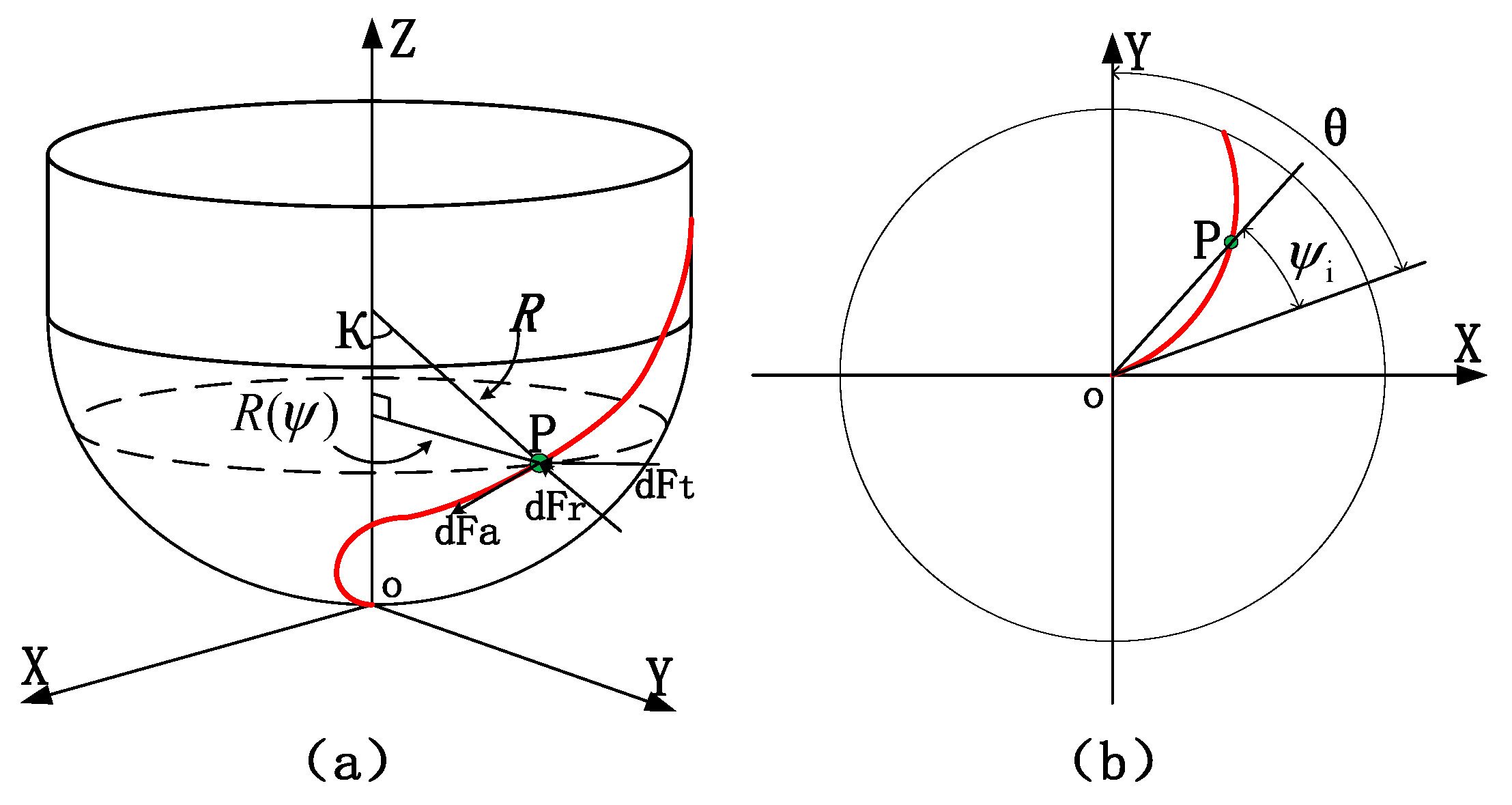
In order to solve the force distribution on the milling cutter and analyze the cutting contact relationship of tool–workpiece, it is necessary to construct the geometric model of the ball-end milling cutter. The cutting edge of the ball-end milling cutter is shown in Figure 2. The coordinate system (O, X, Y, Z) is the machine coordinate system. Point O coincides with the cutter tip and is the origin of the machine coordinate system. Where $R$ is the radius of the ball head, the spiral angle of the tool is ${\beta }_0$, and $\kappa$ is the position angle of any point P on the edge line of the ball head, as shown in Figure 2a. ${\psi }_i$ is the lag angle of any point P on the edge line of the ball head, and $\theta$ is the contact angle of the edge line of the end edge, as shown in Figure 2b.

The ball-end milling cutter’s edge line is formed by the intersection of the hemispherical surface with the same radius and the positive helix surface. The following equation of the ball-end milling cutter’s edge line can be obtained from the geometric relationship in the above figure:

$$x^2+y^2+{\left(z_i-R\right)}^2=R^2,$$

(2)

where $z_i$ is the coordinate of any point P on the ball-end milling cutter in the Z direction, which can be expressed as:

$$z_i={\displaystyle \frac{R{\psi }_i}{\tan {\beta }_0}}.$$

(3)

The radius of the tool’s axial position $z_i$ on the XoY plane is:

$$R^2\left(z_i\right)=x^2+y^2.$$

(4)

Then, the helix lag angle ${\psi }_i$ is:

$${\psi }_i={\displaystyle \frac{z_i\tan {\beta }_0}{R}}.$$

(5)

The contact angle ${\psi }_{ji}$ of the J-th tool tooth at the I-th cutting edge element can be expressed as follows:

$${\psi }_{ji}=\theta -{\psi }_i+\left(j-1\right){\psi }_p,$$

(6)

where $\theta =\omega t=2\pi nt/60$, n is the spindle speed, t is the time, ψ_p is the angle between the teeth of the ball-end milling cutter, and it can be computed by ${\psi }_p=2\pi /N_f$, where $N_f$ is the number of teeth, ${\beta }_0={30}^{°}$.

The arc length of the element can be solved by its position:

$$dS\left({\psi }_i\right)=\sqrt{{\left[R^{\prime }\left({\psi }_i\right)\right]}^2+{\left[R\left({\psi }_i\right)\right]}^2+{\left[z^{\prime }\left({\psi }_i\right)\right]}^2}d\psi .$$

(7)

2.3. Analysis of the Effective Contact Time and Relative Sliding Speed Between the Point on the Blade and the Workpiece

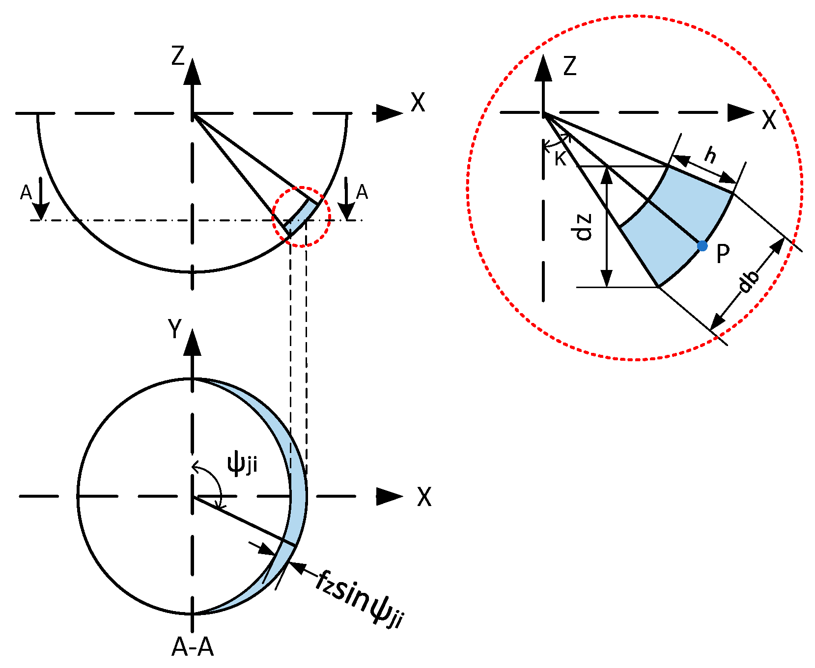
In the milling process, as the tool rotates, the uncut chip thickness changes at all times, which affects the contact area between the tool and the workpiece and also affects the milling force, so the milling force signal usually observed is not constant but a periodic fluctuation. Therefore, to solve the contact relationship between the tool and the workpiece, it is necessary to solve the uncut chip thickness.

Figure 3 shows the geometric characteristics of the cutting element in a two-dimensional coordinate system, where $h$ is the thickness of the normal cutting edge, which is a function of the contact angle ${\psi }_{ji}$ and the axial position angle $\kappa$. The calculation formula is shown as follows:

$$h\left({\psi }_{ji},z_i\right)=f_z\sin {\psi }_{ji}\sin \kappa ,$$

(8)

where $f_z$ is the feed amount of the tool per tooth (mm/z), $\kappa ={\sin }^{-1}{\displaystyle \frac{R\left(z_i\right)}{R}}$, at this time, the undeformed chip width of the cutting edge element is:

$$db={\displaystyle \frac{dz}{\sin \kappa }}.$$

(9)

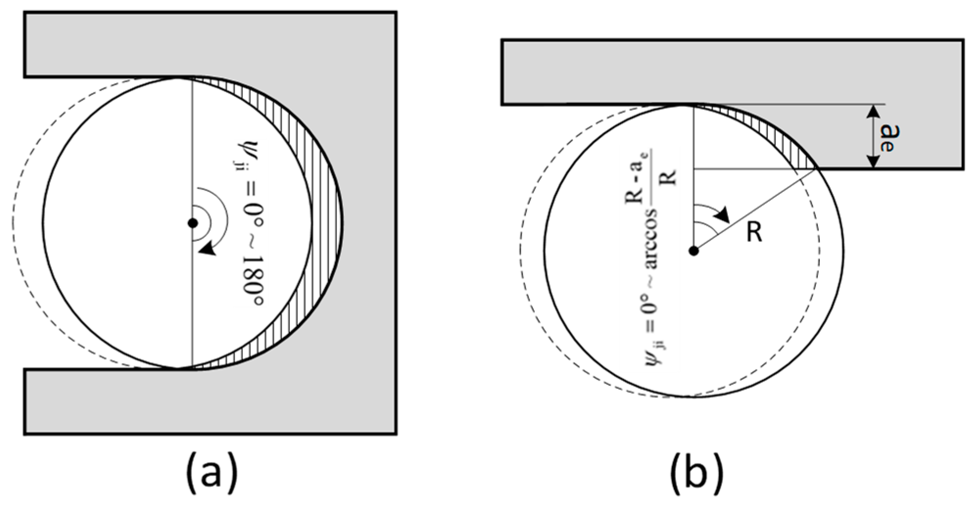
In this paper, the process of cutting edge from cutting into undeformed chips to cutting out is defined as an iterative process. During slot milling, one iteration process is ${\psi }_{ji}$ from 0° to 180°, as shown in Figure 4a, where the shaded part is the workpiece material removed by one iteration process. For side milling, the iterative process is ${\psi }_{ji}$ from 0° to $\arccos \left(R-a_e/R\right)$, as shown in Figure 4b. Where $a_e$ is the radial depth of cut.

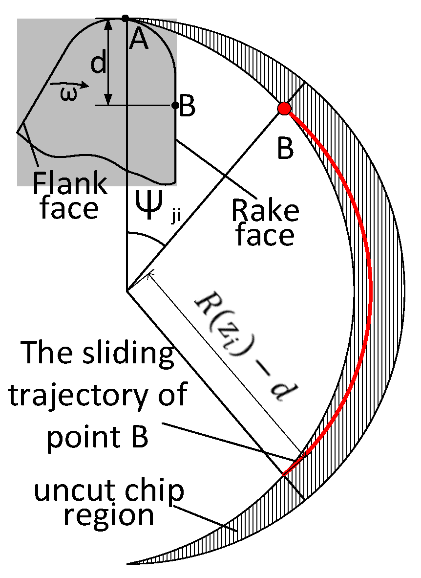
According to the instantaneous uncut chip thickness model mentioned above, combined with the tool cutting workpiece section analysis, it is not difficult to find that in the cutting process, the sliding distance between the different points on the blade of the tool section and the workpiece is different. For example, when ${\psi }_{ji}$ = 0, only the tip of the tool is in contact with the workpiece, and the rest of the points on the blade are in a no-load state. With the rotation of the tool, the uncut chip thickness slowly increases, and more points on the blade are slowly in contact with the workpiece, resulting in relative sliding. Figure 5 shows the contact between the ball-end milling cutter and the workpiece. It can be seen from the figure that during the cutting process, Point A slides relative to the workpiece throughout an iteration. The range of relative sliding between any point B on the front tool surface and the workpiece in one iteration is shown in the red line area in the figure.

It can be seen that the contact time of different tool points with the workpiece in one iteration is different. This period of time is called the effective contact time. Let the distance between any point B on the rake face and the tool tip point in the direction of the rake face be $d$, then when $d=h\left({\psi }_{ji},z_i\right)$, the point contacts the workpiece and slides relative to it.

It is assumed that the first half and the second half of the uncut chip thickness after an iteration are symmetric. According to the geometric relationship analysis, the point on the blade goes through an iteration process, and the effective contact time between point B on the tool and the workpiece is:

$$t={\displaystyle \frac{\pi -2{\psi }_{ji}}{\omega }}.$$

(10)

The relative sliding velocity between the point on the tool section and the workpiece is:

$$V_s=\omega \left[R\left(z_i\right)-d\right].$$

(11)

The relative sliding distance between the point on the tool section and the workpiece is:

$$S=V_{s}t=\left[R\left(z_i\right)-d\right]\left(\pi -2{\psi }_{ji}\right).$$

(12)

2.4. Force Analysis of Iterative Points on the Tool Section

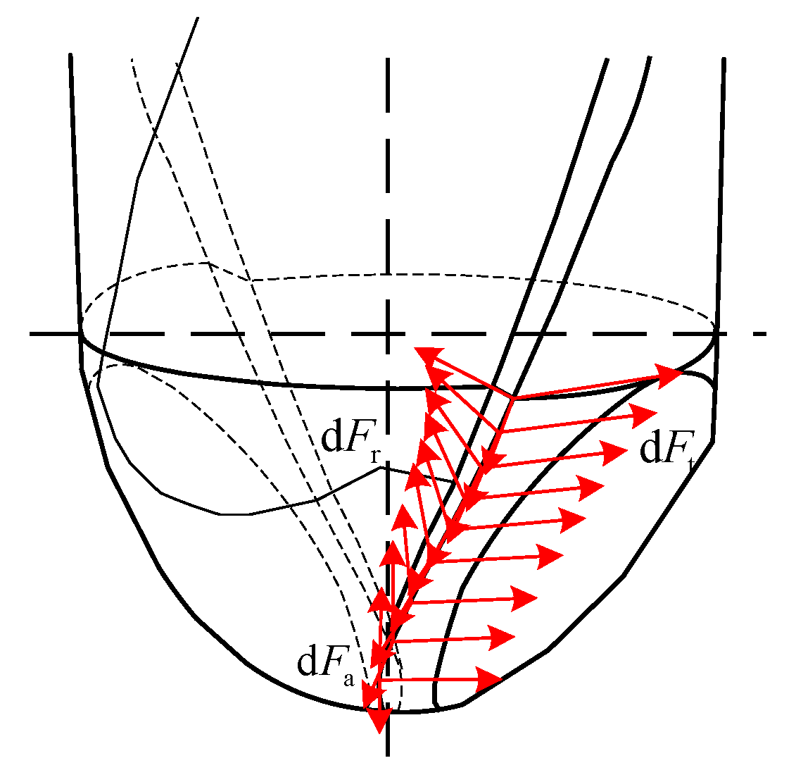
In order to obtain the force of the iteration point of the tool section, the whole force of the tool section must be solved first. According to the milling force model proposed by Lee and Altintas, the cutting edge is first minimized. Figure 6 shows the instantaneous milling force distribution of ball-end milling cutter in single-tooth milling.

In the process of milling, the milling force on the cutting edge is decomposed into components along three directions, which are radial component $d{F}_r$, axial component $d{F}_a$ and tangential component $d{F}_t$. The three components of the cutting edge element can be calculated by the following formula:

$$\left\{\begin{array}{l}d{F}_t=K_{te}ds+K_{tc}{h}_j\left({\psi }_{ji},\kappa \right)db\\ d{F}_r=K_{re}ds+K_{rc}{h}_j\left({\psi }_{ji},\kappa \right)db\\ d{F}_a=K_{ae}ds+K_{ac}{h}_j\left({\psi }_{ji},\kappa \right)db\end{array}\right.,$$

(13)

where $K_{te}{K}_{re}{K}_{ae}$ is tangential, radial and normal ploughing force coefficient, $K_{tc}{K}_{rc}{K}_{ac}$ is tangential, radial and normal shear force coefficient, $ds$ is the arc length of the cutting edge element, $db$ is the corresponding cutting width of the cutting edge element. Since $R$, ${\psi }_{ji}$, ${\psi }_i$ are all functions of $z$, the cutting edge element length $ds$ can be expressed as:

$$dS\left(z\right)=\sqrt{{\left(R\left(z\right){\psi }_i^{\prime }\left(z\right)\right)}^2+{\left(\right(R^{\prime }\left(z\right))}^2+1}.$$

(14)

Then the cutting force element can be expressed as:

$$\left\{\begin{array}{l}d{F}_t=K_{te}dS\left(z\right)+K_{tc}{f}_z\sin {\psi }_{ji}dz\\ d{F}_r=K_{re}dS\left(z\right)+K_{rc}{f}_z\sin {\psi }_{ji}dz\\ d{F}_a=K_{ae}dS\left(z\right)+K_{ac}{f}_z\sin {\psi }_{ji}dz\end{array}\right..$$

(15)

The cutting section is given a certain thickness, so that the thickness of the micro-milling edge is dz, then dz can be given by the following formula:

$$dz={\displaystyle \frac{a_p}{N}},$$

(16)

where $a_p$ is the axial depth of cut, and $N$ is the number of discrete elements of the tool. The sum of the milling forces of the tool in all directions in Equation (18) gives the milling forces of the tool in all directions as follows:

$$\left[\begin{array}{c}{F}_t\\ F_r\\ F_a\end{array}\right]={\sum }_{j=1}^{N_f}{\sum }_{i=1}^N\left[\begin{array}{c}{dF}_t\\ {dF}_r\\ d{F}_a\end{array}\right].$$

(17)

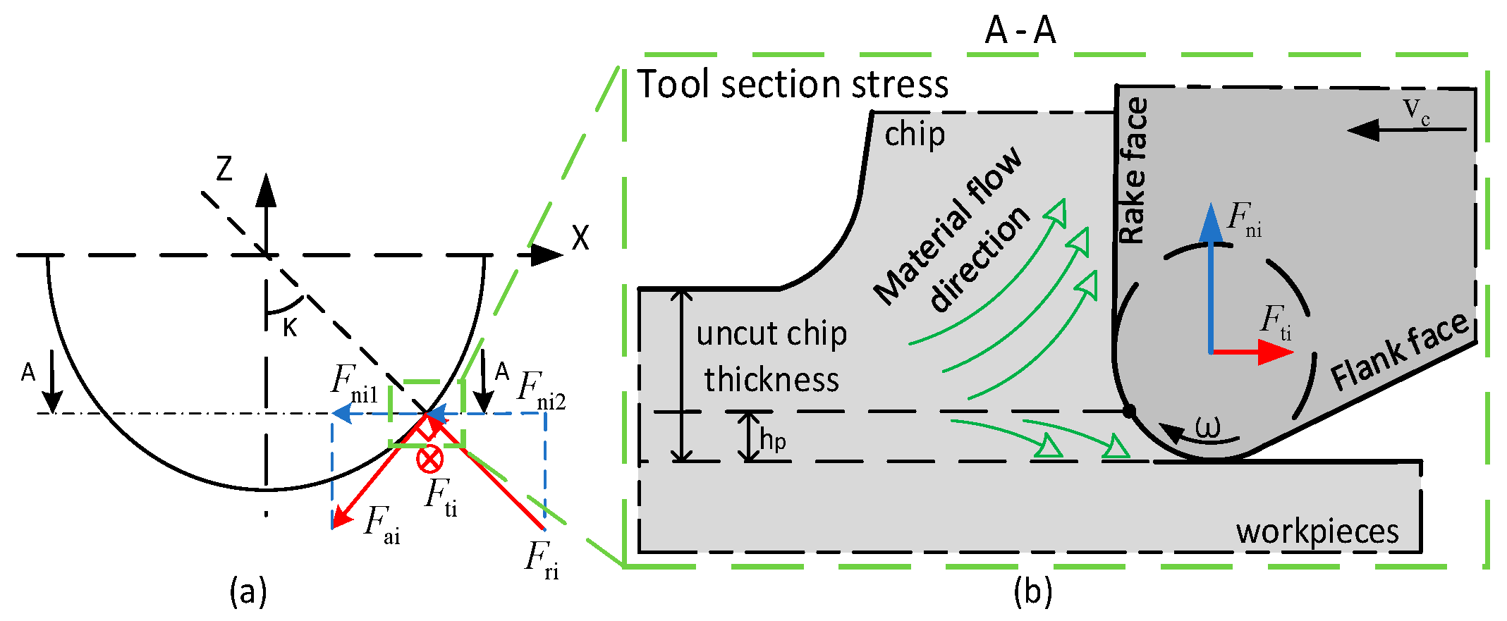
In this paper, the microscopic behavior of wear is analyzed by cutting tool section on the XOY plane. Take any section i as the research object, then the cutting forces which acting on section i are denoted as $F_{ti}$, $F_{ri}$ and $F_{ai}$, as shown in Figure 7a. Where $R_t$ is the radius of the tool tip arc and $\theta$ is the tool tip angle. The force on the section is simplified as the force on $N_p$ points on the section, so that the force on any point k on the section in the three directions is, respectively, $F_{tik}$, $F_{rik}$, $F_{aik}$, then there is the following relation:

$$\left\{\begin{array}{l}{F}_{ti}={\sum }_{k=1}^{N_p}{F}_{tik}\\ F_{ri}={\sum }_{k=1}^{N_p}{F}_{rik}\\ F_{ai}={\sum }_{k=1}^{N_p}{F}_{aik}\end{array}\right..$$

(18)

Since the force of the cross-section is analyzed in this paper, the vertical component of $F_{ai}$ and $F_{ri}$ is ignored, and the resultant force of the lateral component is denoted as $F_{ni}$, as shown by the blue arrow in Figure 7b. It can be seen from the figure that the $F_{ni}$ of the I-th blade section as a whole is:

$$F_{ni}=F_{ri}\sin \kappa +F_{ai}\cos \kappa .$$

(19)

2.4.1. Force Direction Analysis of Iteration Point

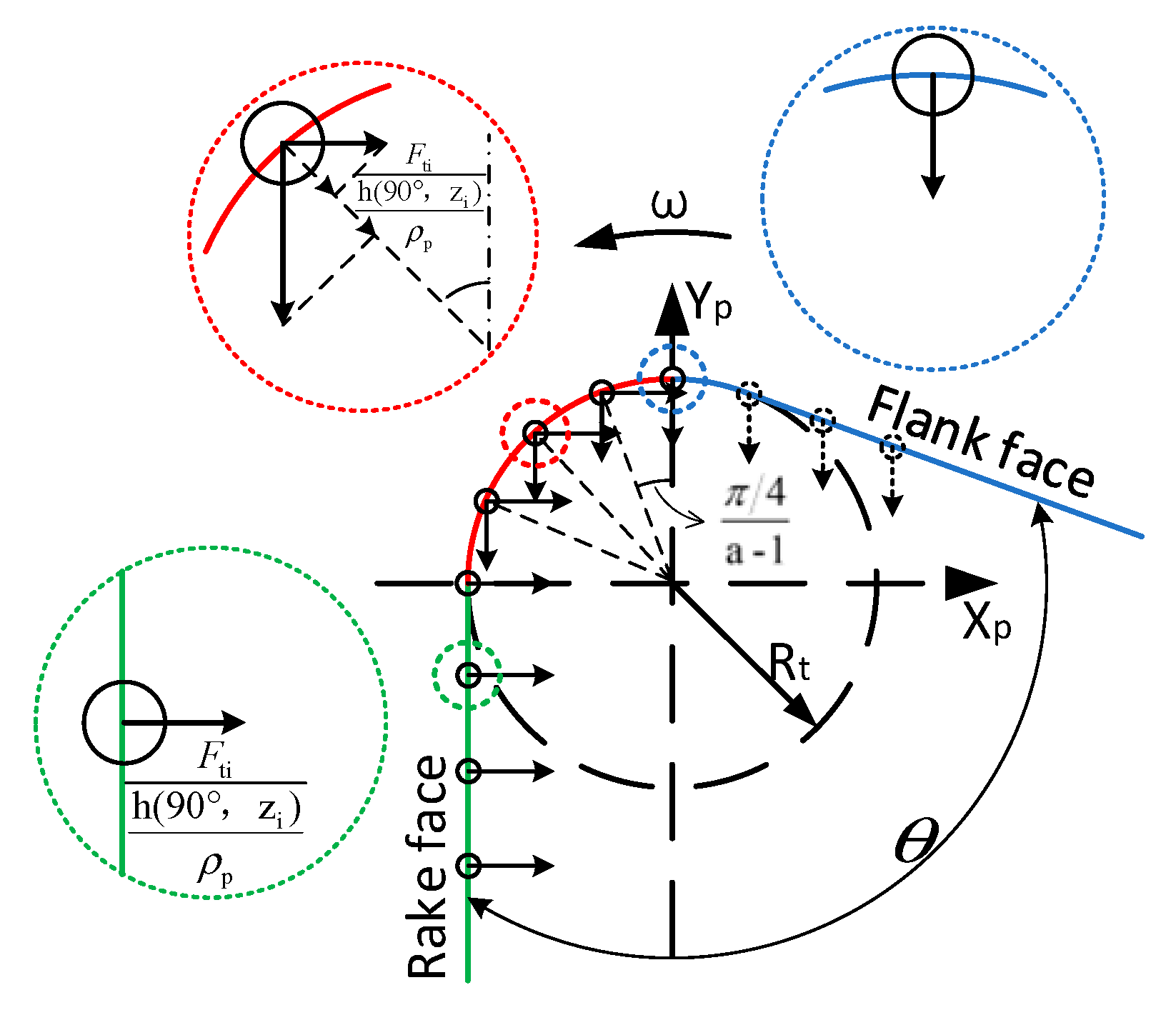
The tangential force $F_{ti}$ and normal force $F_{ni}$ acting on the tool section are assigned to the iteration points on the section. Since the stress conditions of different iteration points on the tool section are different, this paper divides the force of the iteration points into three situations, as shown in Figure 8, according to different positions on the tool section for discussion.

For the points on the rake face, that is, the green area in Figure 8, it can be seen from the force analysis of the iterated points of the tool section in Figure 8 that the points on the rake face are only acted on by tangential force $F_{ti}$, whose direction of action is opposite to the direction of tool rotation.

For the point on the arc of the tool tip, that is, the red area in Figure 8, it is acted on by both the tangential force $F_{ti}$ and the normal force $F_{ni}$, and the direction of the normal force is perpendicular to the direction of the tool rotation.

For the points on the flank face, that is, the blue area in Figure 8, it is only affected by the normal force $F_{ni}$, and when the wear is in the initial stage, only the points in the blue circle in Figure 8 participate in the iteration of the flank face, and the other points gradually join the iteration with the increase in the wear of the flank face.

2.4.2. Calculation of Equivalent Cumulative Milling Force at Iterative Points

In one iteration, the uncut chip thickness gradually increases from zero with the tool rotation and reaches the maximum when the lag angle is ${\psi }_{ji}=90$°, and then gradually decreases. In this process, the force on the tool section changes with the uncut chip thickness, and the contact area between the tool and the workpiece also changes, and the number of stress points will also change. Due to the coupling of chip thickness and the change in tool contact area, it is difficult to calculate the instantaneous force of the iteration points in the cutting process, so it is necessary to introduce the equivalent cumulative milling force of each iteration point after the completion of an iteration.

For the point on the rake face, that is, the iteration point on the green area in Figure 8, assuming that it participates in cutting work when the tool lag angle is from a to b, the equivalent cumulative milling force it receives in one iteration process is:

$$F_n={\int }_a^b{\displaystyle \frac{F_{ti}}{\frac{f_z\sin {\psi }_{ji}\sin \kappa }{{\rho }_p}}}d{\psi }_{ji}.$$

(20)

For the iteration point on the flank face, because it is only affected by the normal force, the equivalent cumulative milling force in the next iteration process can be calculated as:

$$F_n={\int }_a^b{\displaystyle \frac{{dF}_{ri}\sin \kappa +{dF}_{ai}\cos \kappa }{[V_B/{\rho }_p]+1}}d{\psi }_{ji},$$

(21)

where $V_B$ is the width of the flank face wear, and [] indicates downward rounding.

For the point on the arc of the tool tip, it can be seen from the above that it is subject to tangential force and normal force, and the equivalent cumulative tangential force on it in one iteration process is the same as that on the point on the rake face. According to the geometric relationship analysis, the equivalent cumulative normal force on one iteration process can be calculated as follows:

$${\sigma }_n={\int }_a^b\sin \left(k{\displaystyle \frac{{\rho }_p}{2R_t}}\right){\displaystyle \frac{F_{ti}}{\frac{f_z\sin {\psi }_{ji}\sin \kappa }{{\rho }_p}}}+\cos \left(k{\displaystyle \frac{{\rho }_p}{2R_t}}\right){\displaystyle \frac{{dF}_{ri}\sin \kappa +{dF}_{ai}\cos \kappa }{[V_B/{\rho }_p]+1}}d{\psi }_{ji},$$

(22)

where k represents the k-th point on the tool tip arc from $Y_p$ axis to $X_p$ negative half axis number in the tool section coordinate system.

At this time, the normal force of the point on the section is obtained, and the wear volume can be calculated according to the cutting tool wear rule formula. As the tool is processed for longer and longer, the volume of wear will gradually increase. Cutting tool wear will go through three stages: initial wear, normal wear, and sharp wear.

2.5. Cutting Temperature Analysis of Tool Section

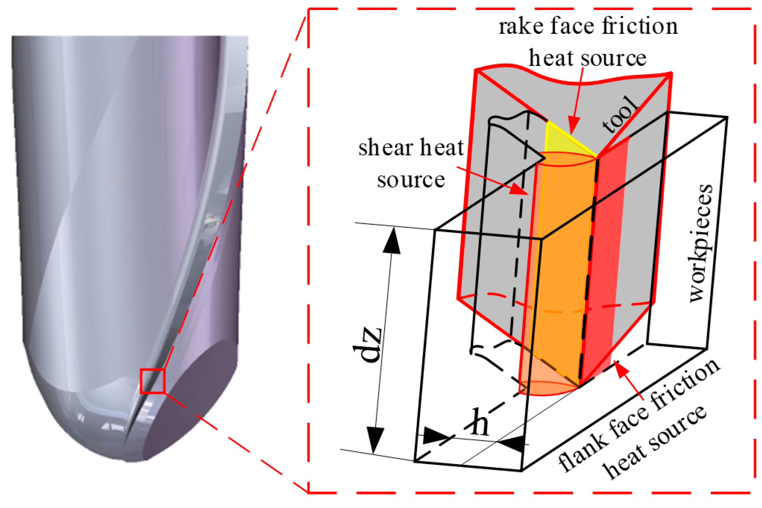
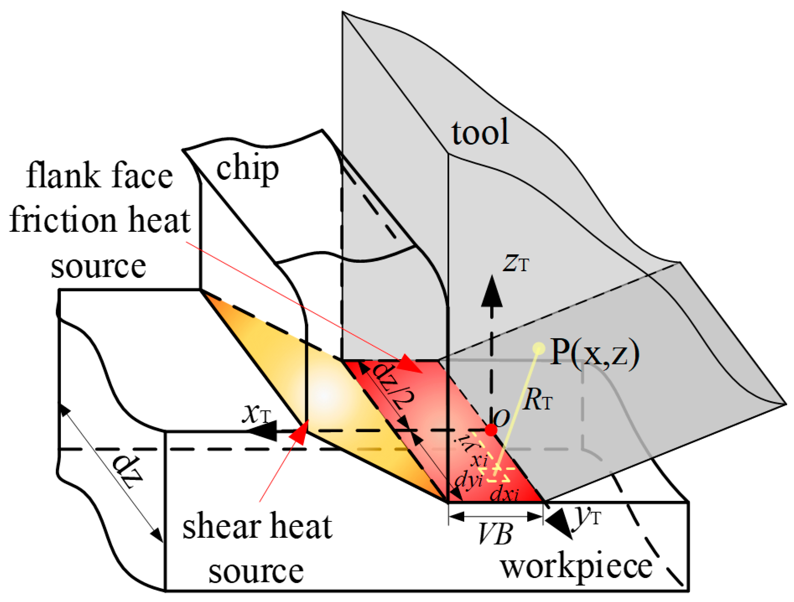
It can be seen from the proposed wear rate model that the cutting temperature also has a certain effect on the wear rate, so it is necessary to analyze the heat production of the machining system. Because the axial direction of the milling cutter is miniaturized in this paper, the micro-milling process can be regarded as an orthogonal cutting, as shown in Figure 9. There are three main sources of heat generated by the cutting system: (1) the heat generated by the shear deformation of the material, as shown in the orange area in the figure; (2) heat generated by friction between the rake face and the bottom surface of the chip (yellow area); (3) heat generated by friction between the flank face and the machined surface (red area).

Since most of the heat generated by shearing is discharged with the chips, only part of the heat can be transferred to the tool, so the temperature of the tool is mainly affected by the heat source of the rake face and flank face, and the shear heat source is no longer analyzed separately. According to the thermodynamic model proposed by Wenlin Li [30], the temperature at any point on the tool can be given by the following formula:

$$T_f\left(a,b\right)=T_{rake}\left(a,b\right)+T_{flank}\left(a,b\right)+T_0,$$

(23)

where $T_{rake}\left(a,b\right)$ is the temperature rise caused by the rake face heat source, $T_{flank}\left(a,b\right)$ is the temperature rise caused by the flank face heat source, and $T_0$ is the initial temperature. Based on the thermodynamic model proposed by Wenlin Li, this paper will make some changes to make it suitable for milling conditions so as to solve the machining temperature of the iterative point of the tool.

2.5.1. Heat Transfer of the Rake Face Heat Source

Figure 10 shows the heat transfer diagram of the rake face, where $dz$ is the width of the rectangular heat source on the rake face.

Since the uncut chip thickness changes with the time of tool rotation during milling, the average equivalent chip thickness is introduced as the length of the rectangular heat source. The average equivalent chip thickness $h_{av}$ is calculated by the following formula [17]:

$$h_{av}=R+f_z\sin {\psi }_{ji}-\sqrt{R^2-f_z^2\cos {\psi }_{ji}}.$$

(24)

The coordinate system of the heat transfer system is established by taking the midpoint of the upper boundary of the rectangular heat source as the origin. Since the rake face heat source appears between the rake face and the chip bottom surface, it is necessary to consider the heat taken away by the chip during the heat production process. Assuming that the proportion of heat taken away by the chips is $B_1\left(x\right)$, the proportion of effective heat remaining on the rake face is $1-B_1\left(x\right)$ of the total heat production on the front cutter surface. The calculation of $B_1\left(x\right)$ is given by the following formula [31]:

$$B_1\left(x\right)=\left(B_{chip}-\Delta B\right)+2\Delta B{\left({\displaystyle \frac{x}{h_{av}}}\right)}^{m_1}+C\Delta B{\left({\displaystyle \frac{x}{h_{av}}}\right)}^{k_1},$$

(25)

where $B_{chip}$ is the average distribution fraction of chip heat obtained by matching the average temperature rise at the contact interface of the two sides, $\Delta B$ is the maximum compensation of $B_{chip}$ at both ends of the interface heat source. The temperature rise at any point of the tool caused by the friction heat source of the rake face is given by the following formula [31]:

$$T_{rake}^{friction}\left(a,b\right)={\displaystyle \frac{1}{\pi {\lambda }_t}}{\int }_{y_i=-{\displaystyle \frac{dz}{2}}}^{{\displaystyle \frac{dz}{2}}}{\int }_{x_i=0}^{h_{av}}\left\{q_{rake}^{friction}\left(x_i\right)\left[1-B_1\left(x_i\right)\right]{\displaystyle \frac{1}{R_i}}\right\}d{x}_{i}d{y}_i.$$

(26)

The temperature rise caused by the shear heat source passing through the rake face to the tool is:

$$T_{rake}^{transfer}\left(a,b\right)={\displaystyle \frac{q_{rake}^{transfer}}{\pi {\lambda }_t}}{\int }_{y_i=-{\displaystyle \frac{dz}{2}}}^{{\displaystyle \frac{dz}{2}}}{\int }_{x_i=0}^{h_{av}}\left\{\left[1-B_1\left(x_i\right)\right]{\displaystyle \frac{1}{R_i}}\right\}d{x}_{i}d{y}_i.$$

(27)

The tool temperature rise caused by the rake face is:

$$T_{rake}\left(a,b\right)=T_{rake}^{friction}\left(a,b\right)+T_{rake}^{transfer}\left(a,b\right).$$

(28)

In the above formula, $q_{rake}^{friction}$ is the heat generated by the friction of the rake face, $q_{rake}^{transfer}$ is the heat transferred from the shear heat to the rake face, ${\lambda }_t$ is, $R_i=\sqrt{{(x-x_i)}^2+y_i^2+z^2}$ is the distance between the point in the tool and the element of the heat source.

2.5.2. Heat Transfer of the Flank Face Heat Source

In the same way as the rake face heat source, as shown in Figure 11, the heat source generated by the friction of the flank face also has two directions: the tool and the workpiece.

Assuming that the heat proportion of the incoming workpiece is $B_2\left(x\right)$, the heat proportion of the incoming tool is $1-B_2\left(x\right)$. The calculation of $B_2\left(x\right)$ is given by the following formula:

$$B_2\left(x\right)=\left(B_{tool}-\Delta B\right)+2\Delta B{\left({\displaystyle \frac{x}{VB}}\right)}^{m_2}+C\Delta B{\left({\displaystyle \frac{x}{VB}}\right)}^{k_2}$$

(29)

where $B_{tool}$ is the average distribution fraction of the tool heat. The temperature rise of any point of the tool caused by the friction heat source of the flank face is shown as follows:

$$T_{flank}^{friction}\left(a,b\right)={\displaystyle \frac{1}{\pi {\lambda }_t}}{\int }_{y_i=-{\displaystyle \frac{dz}{2}}}^{{\displaystyle \frac{dz}{2}}}{\int }_{x_i=0}^{VB}\left\{q_{flank}^{friction}\left(x_i\right)\left[1-B_2\left(x_i\right)\right]{\displaystyle \frac{1}{R_i}}\right\}d{x}_{i}d{y}_i$$

(30)

The temperature rise caused by the shear heat source passing through the flank face to the tool is:

$$T_{flank}^{transfer}\left(a,b\right)={\displaystyle \frac{q_{flank}^{transfer}}{\pi {\lambda }_t}}{\int }_{y_i=-{\displaystyle \frac{dz}{2}}}^{{\displaystyle \frac{dz}{2}}}{\int }_{x_i=0}^{VB}\left\{\left[1-B_2\left(x_i\right)\right]{\displaystyle \frac{1}{R_i}}\right\}d{x}_{i}d{y}_i$$

(31)

The tool temperature rise caused by the flank face is:

$$T_{flank}\left(a,b\right)=T_{flank}^{friction}\left(a,b\right)+T_{flank}^{transfer}\left(a,b\right)$$

(32)

2.6. Wear Iteration Mode

According to the above analysis and calculation, the force, temperature, and contact relationship with the workpiece on the tool section can be obtained. According to the wear rate model proposed in Section 2.1, the wear rate of each iteration point on the tool section can be solved. From the above contact relation analysis, it can be seen that the effective contact time of different points in one iteration is different from that of points at different positions in one iteration. Thus, the volume of tool material peeled off by iteration points on the cross-section in one iteration can be calculated. It is assumed that after each iteration, the tool section will form a hemispherical volume loss with the iteration point as the center of the sphere. In this paper, this volume loss is called crater wear, and the radius of the crater wear is recorded as $R_l$, and its calculation formula is as follows:

$$R_l=\sqrt[3]{{\displaystyle \frac{3w}{2\pi }}}.$$

(33)

With each iteration of the tool section, crater wear will expand with the iteration point as the center of the sphere so that the radius will change. The crater wear radius after n iterations is given by the following formula:

$$R_l=\sqrt[3]{{\displaystyle \frac{3{\sum }_{i=1}^n{w}_i}{2\pi }}},$$

(34)

where $w_i$ is the wear volume of the i-th iteration. Wear iterative calculation is carried out for each iteration point, and the wear region of each iteration point on the section is overlapped; then the section iterative wear region, as shown in Figure 12 can be obtained. Based on this, all the sections of the tool are overlapped to obtain the prediction results of the 3DWM of the tool.

3. Experimental Details

To verify the feasibility of the proposed model, milling experiments were conducted on TiAl alloy using carbide ball-end mills. The wear morphology of the ball-end mills after processing was examined microscopically. The experiment adopts the intermittent cutting method; the total is divided into 30 cuts, and the linear feed is done on the workpiece. After each cut is completed, the tool is removed from the machine tool, and the tool wear morphology is detected with the ultra-depth microscope. No coolant is added to the cutting process. To simplify the experimental verification process, this paper selects any specific layer of the milling cutter and uses the proposed wear rate model to predict the wear morphology on the selected tool cross-section, specifically calculating the wear depth of the points on the selected cross-section. The wear depth of the corresponding cross-section of the milling cutter that completed the corresponding milling work in the experiment is compared with the calculated value of the model to verify the accuracy of the model.

3.1. Experimental Equipment

As shown in Figure 13, the milling machine used for the milling experiment is a CAMUMC850 three-axis milling machine. The cutting tool is a double-edged solid carbide ball-end mill (DV-OCSB2100-L140 DIJET, Ōsaka, Japan) from Dajie, with a diameter of 10 mm. The helix angle of the tool is 30° and its Vickers hardness is 1830 HV. The workpiece is in the shape of a cylindrical bar with a diameter of 74.8 mm and a length of 199 mm. Its physical properties are shown in

Table 1. Physical properties of materials.

E (GPa)	ρ (g/cm3)	λ (W/m °C)	HV	δ (%)
110	4.85	8.6	317	11

.

3.2. Experimental Parameters

The cutting experiment parameters are shown in

Table 2. Experimental parameters.

${\mathit{v}}_{\mathit{c}}$ (m/min)	$\mathit{f}$ (mm/r)	${\mathit{a}}_{\mathit{p}}$ (mm)	n (r/min)
90	0.15	0.5	8000

. The tool is taken out after cutting for a period of time under the following working conditions, and the wear of the tool is observed by ultra-depth of field optical microscope (VHX-1000, Keyence, Ōsaka, Japan).

The area in which the tool participates in cutting is divided into 10 micro-elements according to the direction of the tool axis, and the tool section of layer 7 is selected. It can be seen from [3] that according to the regression analysis of simulation and experimental results, the constants A and B in the wear rate model are 0.0468 mm²/min and 97.8 mm/min, respectively, and the value of E/R is 7883 K. By substituting these coefficients into the wear rate model, the wear rate at different points on the blade can be calculated.

4. Result and Discussion

Figure 14 shows the wear of the milling cutter under different milling times, where the yellow line is the original shape of the blade, and the white dashed line is the wear of the tool section. As can be seen from the figure, the wear on the front tool face near the tip of the tool is the most severe. With the increase in milling time, the wear range gradually expands, and the most severe wear on the front tool face occurs at a certain distance from the cutting edge.

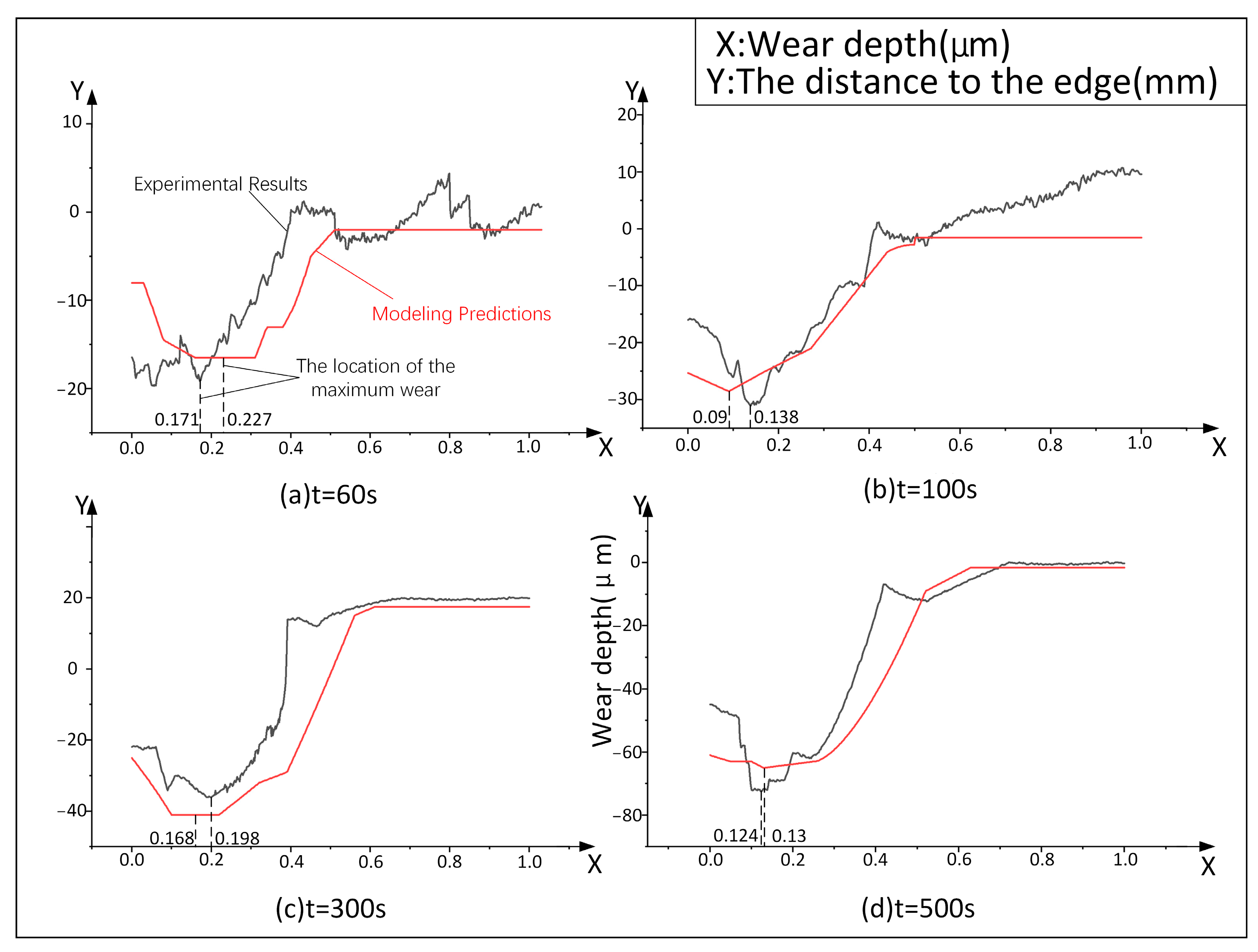
In order to verify the accuracy of the model, the experimental results of the tool wear of the rake face were compared with the calculated values of the model, and the comparison results were as follows:

The above figure shows the comparison between the rake face wear of the tool after different working periods and the calculated results of the model. The ordinate in the figure is the wear depth of the front tool face. The horizontal coordinate is the distance from the tip of the blade. The black lines are experimental data. The red lines are the results of the proposed model.

As can be seen from Figure 15, the trend of experimental data and model calculation results is roughly the same. When the cutting time is 60 s, the average wear depth of the rake face is 5.7 μm in the experimental data and 7.2 μm in the model calculation. When the cutting time is 100 s, the experimental data are basically consistent with the trend calculated by the model within 0.6 mm from the tool tip, and the difference becomes larger after 0.6 mm. Within 0.6 mm, the average wear depth of the front tool surface of the experimental data is 13.2 μm, and that calculated by the model is 11.6 μm. When the cutting time reaches 300 s, the average wear depth of the front tool surface is 19.5 μm in the experimental data and 27.6 μm in the model calculation. When the cutting time reaches 500 s, the average wear depth of the front tool surface in the experimental data is 24 μm, and the model calculation is 28.6 μm. By adding the experimental average and the calculated average of the four time periods, the accuracy of the model calculation is 83.2%. The square root error RMSE is calculated for the experimental and simulation data in four time periods, and the error values are 3.345, 4.501, 8.001, and 7.434, respectively. It can be concluded that the accuracy of the calculation results on the wear amount of the model is high. However, when the machining time is short, the error of the fitting degree of wear morphology is larger, and the fitting degree increases with the increasing of time. It can be seen that there is a certain gap between the model and the experimental results. Factors such as chatter and wear between different teeth can be ignored in the calculation of the model, but these factors cannot be avoided in the actual machining process. This is the main reason for the separation between model and experiment.

It can be imagined that if the above problems can be solved in this research direction in the future, the accuracy of the model can be improved and the 3DWM of the tool can be accurately predicted. This technology can be used to detect tool wear during machining. Combined with a big data algorithm, this technology is embedded in CNC to detect the wear of different parts of the tool in real time. Adjust the tool position according to the wear condition, reduce the impact of the tool wear on the machining quality, and improve the utilization rate of the tool.

5. Conclusions

Based on the wear rate model, this paper developed a 3DWM prediction model for ball-end milling cutter. Through model calculation and experimental analysis, the following conclusions were obtained:

Based on the analysis of normal stress, relative slip, and cutting temperature, the model incorporates the influence factors of tool wear. The anticipated outcome for predicting the front tool wear is as follows: the most severe wear region occurs at a specific distance from the cutting edge, which aligns with actual machining conditions.

The results indicate that an increase in cutting time correlates with a greater wear depth on the front tool face. When predicting wear depth, the model’s calculated values demonstrate an accuracy of 83.2% in comparison to experimental data.