Abstract
To accurately assess the seismic risk of bridges, this study systematically conducted probabilistic seismic hazard–fragility–risk assessments using a reinforced concrete continuous girder bridge as a case study. First, the CPSHA method from China’s fifth-generation seismic zoning framework was employed to calculate the Peak Ground Acceleration (PGA) with 2%, 10%, and 63% exceedance probabilities over 50 years as 171.16 gal, 98.10 gal, and 28.61 gal, respectively, classifying the site as being with 0.10 g zone (basic intensity VII). Second, by innovatively integrating the Response Surface Method with Monte Carlo simulation, the study efficiently quantified the coupled effects of structural parameter and ground motion uncertainties, a finite element model was established based on OpenSees, and the seismic fragility curves were plotted. Finally, the risk probability of seismic damage was calculated based on the seismic hazard curve method. The results demonstrate that the study area encompasses 46 potential seismic sources according to China’s fifth-generation zoning. The seismic fragility curves clearly show that side piers and their bearings are generally more susceptible to damage than middle piers and their bearings. Over 50 years, the pier risk probabilities for the intact, slight, moderate, severe damage, and collapse are 68.90%, 6.22%, 15.75%, 7.86%, and 1.27%, while the corresponding probabilities of bearing are 3.54%, 44.11%, 25.64%, 7.74%, and 18.97%, indicating significantly higher bearing risks at the moderate damage and collapse levels. The method proposed in this study is applicable to various types of bridges and has high promotion and application value.
1. Introduction
China is located at the intersection of the Circum-Pacific Seismic Zone and the Eurasian Seismic Zone, making it one of the countries most severely affected by earthquake disasters globally [1]. The 1976 Tangshan earthquake nearly destroyed all highway and railway bridges in Tangshan City. The 2008 Wenchuan earthquake caused severe damage or collapse to 25 highway bridges in Sichuan Province. Notably, the G213 Baihua Bridge, located approximately 1.0 km from the Longmenshan active fault, experienced the collapse of its fifth span, with 90% of the remaining piers exhibiting crushing failures [2]. With the arrival of active cycles, future earthquakes may cause even more severe bridge damage. Therefore, systematically analyzing the failure mechanisms and damage degrees of bridges under different ground motions is crucial for improving seismic capacity of bridges and ability of regional disaster mitigation.
The degree of bridge seismic damage depends on two aspects. First, the intensity and probability of seismics at the bridge site (study site), which belongs to seismic hazard assessment. Factors such as seismic zones, distribution of potential seismic source zones, historical seismic records and site conditions may affect seismic hazards. Second, the seismic performance of the bridge itself, characterized by the probability of exceeding various damage levels under a given ground motion, which belongs to seismic fragility assessment, may affect seismic hazards. Factors such as bridge structural form, construction quality and protective measures influence seismic fragility. The probability of bridge seismic risk, which represents the probability of a specific bridge exceeding various damage levels over a certain period [3], is derived from the integration of seismic hazard and fragility assessments by analyzing their coupled characteristics.
Numerous scholars have made significant contributions to the field of structural seismic risk assessment. In the field of seismic hazard assessment, Cornell proposed the Probabilistic Seismic Hazard Analysis (PSHA) [4]. China’s current seismic hazard assessment methodology (CPSHA) was developed based on PSHA [5]. The third to fifth generations of China’s seismic ground motion zonation schemes were formulated by CPSHA [6]. For seismic fragility assessment, Vamvatsikos and Cornell introduced the Incremental Dynamic Analysis (IDA), which has since become the most widely adopted method [7]. Wang et al. proposed a fragility assessment approach that incorporated multi-dimensional performance limit states and pioneered fragility curves for multi-span continuous concrete girder bridges, explicitly accounting for pier ductility and lateral deformation [8]. Li et al. established the probability density evolution theory and applied it to nonlinear dynamic response analysis, thereby quantifying the variability in physical parameters of engineering structures [9]. In seismic risk assessment, Yin et al. and Che et al. employed the Monte Carlo method and seismic hazard curve method to assess seismic risks for a highway embankment and proposed a risk management method based on risk acceptability theory [10,11]. Abeysiriwardena et al. developed a seismic risk analysis method for RC frame structures considering aftershock effects [12]. Their work involved convolving mainshock–aftershock fragility functions with hazard functions, extending the traditional risk integral formula to a bivariate domain, and deriving demand risk functions incorporate aftershock impacts.
Structural uncertainties are inherent in the design, construction and operation of bridges. A critical technical challenge lies in characterizing the coupled effects of structural parameter and ground motion uncertainties on bridge seismic performance. Although Chinese seismic design philosophy for bridges adheres to the principle of “no damage under minor seismic events, repairable damage under moderate seismic events, and no collapse under major seismic events” [13], clear definitions are lacking for the corresponding seismic intensity indicators (“minor”, “moderate” “major” and damage states (“no damage”, “repairable” “no collapse”); this ambiguity significantly limits the practical application of the philosophy. To address these issues, primary contributions of this study are twofold: (1) to develop an integrated probabilistic framework for bridge seismic risk assessment; (2) to introduce a novel, computationally efficient methodology that integrates the Response Surface Method with Monte Carlo simulation to effectively quantify the coupled effects of structural and ground motion uncertainties. This integrated approach thereby provides a practical and theoretically sound tool for performance-based seismic design and decision-making. The study flowchart is shown in Figure 1.
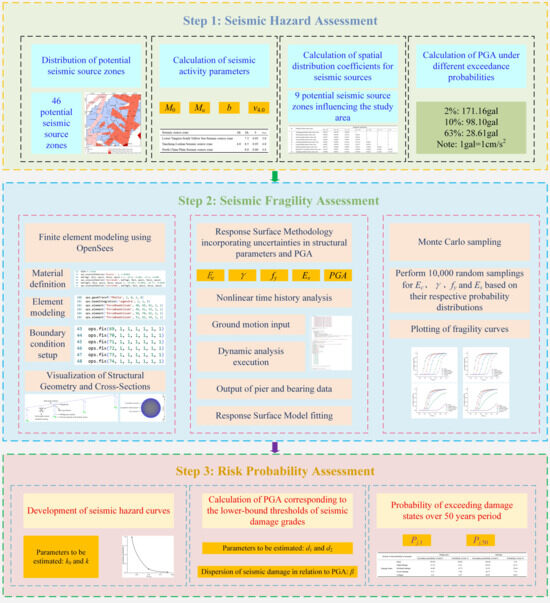
Figure 1.
Study flowchart.
2. Finite Element Model Development of the Study Object
The bridge studied is located in Boshan District, Zibo City, Shandong Province, China, with a span arrangement of 3 × 30 m. The main beam was constructed with C50 concrete (The 28-day compressive strength of the concrete is 50 MPa), while the bridge piers and bent caps were constructed using C40 concrete (the 28-day compressive strength of the concrete is 40 MPa). HRB400 steel (the tensile strength of the reinforcing steel is 400 MPa.) was adopted for reinforcement, and pot rubber bearings were employed as supports. In the finite element modeling using OpenSees (Open System for Earthquake Engineering Simulation), the main beam and bent caps were modeled with elastic beam-column elements, the bearings were simulated using zero-length elements, the bridge piers were represented by force-based beam-column elements with fixed bases at the foundation. Given that the bridge site is characterized by stiff soil (Site Class II), where soil–structure interaction effects are known to be minimal, this fixed-base assumption is considered appropriate, allowing the analysis to focus on the uncertainty and performance of the superstructure components. Concrete in the bridge piers was modeled with the Concrete01 material, and reinforcing steel was characterized by the Steel02 material [14,15,16]. The constitutive relationships of the Concrete01 and Steel02 materials are shown in Figure 2. Figure 2 is cited from the official OpenSees website at: https://opensees.berkeley.edu/ (accessed on 27 April 2024)
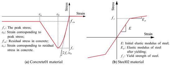
Figure 2.
Constitutive relationships of material.
The piers were discretized into fiber elements, which were partitioned using Legendre integration. Each element was divided into five integration points along its longitudinal axis, with each integration point having the same cross-section. The five Legendre integration points along the longitudinal direction of the pier and the division of fibers at their cross-sections are shown in Figure 3.
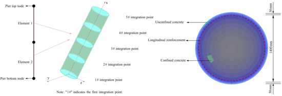
Figure 3.
Legendre integration points and the fiber division of their cross-sections.
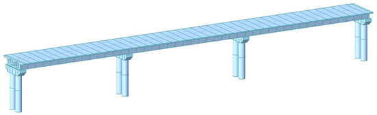
Figure 4.
Midas finite element model of bridge.
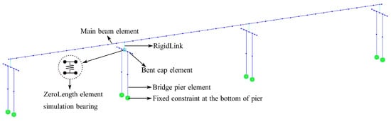
Figure 5.
OpenSees finite element model of bridge.
3. Classification of Bridge Seismic Damage Levels and Selection of Damage Parameters
3.1. Classification of Bridge Seismic Damage Levels
The Standard for Classification Seismic Damage to Buildings and Structures (GB/T 24335-2009) [17] classify the seismic damage into five levels: intact, slight damage, moderate damage, severe damage and collapse [18]. This study adopts this classification for bridge and provides qualitative descriptions for each damage level, as summarized in Table 1.

Table 1.
Qualitative descriptions of bridge seismic damage levels.
3.2. Seismic Damage Parameters for Bridges
Bridge piers and bearings are the primary components susceptible to seismic damage. Accordingly, separate damage parameters were selected for each to assess their performance independently.
3.2.1. Seismic Damage Parameters of Bridge Piers
Due to their nonlinear response characteristics, which are mainly governed by flexural damage [19], the displacement ductility ratio was selected as the seismic damage parameter for bridge piers in this study [20]. The calculation method is shown in Equation (1).
where μd is the displacement ductility ratio of the pier, Δd is the relative displacement of the pier top, and Δcy1 is the relative displacement at the pier top when the outermost longitudinal reinforcement steel first yields. The relationship between the bridge seismic levels and μd is summarized in Table 2.
Table 2.
Relationship between bridge seismic damage levels and μd.
Where μcy1 is the displacement ductility ratio at the first yield of the outermost longitudinal reinforcement in the bridge pier. μcy is the equivalent displacement ductility ratio, defined as the ratio of the ultimate displacement to the yield displacement of the bridge pier, where a higher value indicates superior ductility. μc4 represent the displacement ductility ratio when the compressive strain of the cover concrete reaches 0.004, which corresponds to the stage of complete spalling of cover concrete and initiation of crake in the core concrete region. Finally, μcmax is the maximum ductility ratio, attained when the core concrete crushes, the longitudinal reinforcing steel yields, and the stirrups fracture. Since μcy1 only accounts for the initial yield and ignores the subsequent nonlinear deformations, it is defined as μcy1 = 1. The calculation methods for μcy, μc4 and μcmax are shown in Equation (2)–(4) [21].
where φy1 denotes the curvature at the first yield of the outermost longitudinal reinforcing steel in the bridge pier. φy2 is the equivalent yield curvature, and φc4 is the curvature when the compressive strain of the cover concrete reaches 0.004. L denotes the height of the bridge pier. fy is the yield strength of the reinforcement steel. ds is the diameter of the steel. This study adopted the following parameter values: φy1 = 8.164 × 10⁻⁴ rad/m, φy2 = 9.233 × 10⁻⁴ rad/m, φc4 = 3.421 × 10⁻³ rad/m, L = 10 m, fy = 400 MPa and ds = 0.03 m. Based on these calculations, Table 2 was converted to Table 3.
Table 3.
Relationship between bridge seismic damage levels and μd.
3.2.2. Seismic Damage Parameters of Bearings
Due to the relatively low horizontal displacement threshold of pot rubber bearings, this study selected the shear deformation d as the seismic damage parameter for bearings, following the research by Zhong et al. [22]. The relationship between bridge seismic damage level and d is shown in Table 4.
Table 4.
Relationship between bridge seismic damage levels and d.
4. Probabilistic Seismic Hazard Assessment of the Study Site
4.1. Overview of the CPSHA Method
(1) The methodology adopted the principle of three-level potential seismic source zone division and constructed the corresponding seismic activity model. This model comprises seismic statistical zones (seismic zones) and potential seismic source zones of background seismic activity (background sources), and potential seismic source zones of tectonic structures (tectonic sources), which are spatially superimposed [23]. The seismic statistical zone serves as the bottom layer and the statistical unit for seismic activity parameters. The background source, as the middle layer, reflects the characteristics of background seismic activity within the seismic zones and differences in seismic tectonic models. The tectonic source, as the top layer, reflects the characteristics of moderate-to-strong seismic activities associated with local tectonic structures. The representation of spatial inhomogeneity in seismic activity varies across different magnitude ranges: for small-to-moderate magnitudes, it is jointly represented by tectonic sources and background sources, whereas for moderate-to-strong magnitudes, it is represented solely by tectonic sources.
(2) The seismic magnitudes in seismic zone follow the Gutenberg–Richter relationship, as shown in Equation (5) [24].
where N is the number of earthquakes with magnitudes greater than or equal to M, M is the seismic magnitude; M0 is the threshold magnitude, defined as the minimum magnitude that causing damage; Mu is the magnitude upper limit, which is the maximum possible seismic magnitude; a and b are statistical parameters, where a reflects the level of seismic activity over a specific period, and b reflects the proportional relationship between large and small earthquakes. The probability density function of the magnitude distribution in seismic zones can be derived from Equation (5), as shown in Equation (6) [25].
where β = b·ln10.
(3) The seismic activity in a seismic zone over a period follows a Poisson distribution, implying that the probabilistic characteristics of seismic activity in the zone can be determined by a parameter v. The two-state Poisson model assumes that seismic activity in the seismic zone has “active” and “inactive” states, making it more consistent with the actual occurrence pattern of earthquakes. The probability PK of K earthquakes occurring in the seismic zone over the next T years as shown in Equation (7) [26].
(4) Seismic activity within a seismic zone is non-uniformly distributed, whereas it is uniformly distributed within a potential seismic source zone. The probability that an earthquake in magnitude bin mj occurs in the i-th potential seismic source zone is denoted as fi,mj. Given that the area of the i-th potential seismic source zone is Ai, the probability P(mj|i) of an earthquake in magnitude bin mj occurring at any point within the i-th potential seismic source zone as shown in Equation (8) [27].
(5) Equation (9) was derived based on Equation (5) to Equation (8).
where P(mj) is the probability that an earthquake within the seismic zone lies within the magnitude bin mj ± 0.5Δm, and sh(β·Δm/2) denoted the hyperbolic function with β·Δm/2 as its argument. Assuming that an earthquake of magnitude mj occurs randomly in the k-th seismic zone, the probability of generating a PGA ≥ yq at a given site is expressed by Equation (10).
where Nm is the total number of magnitude bins, Nks is the number of potential seismic source zones in the k-th seismic zone, yq is the specified PGA value, and dxdy is the cell area of the gridded potential seismic source zones. By integrating the effects of Nz seismic zones in the area using the total probability formula, the seismic hazard probability can be calculated using Equation (11).
(6) The PGA attenuation relationship shown in Equation (12) is adopted [28].
where M is the surface wave magnitude, R is the epicentral distance, and A, B, C, D and E are coefficients, with values shown in Table 5.
Table 5.
Coefficients of the PGA attenuation relationship.
Where the Long axis refers to the principal direction in the spatial distribution of ground motion parameters, along which these parameters vary gradually and exhibit a wider zone of influence. That is, ground motion parameter attenuation along the Long Axis occurs at relatively low gradient with increasing distance from the seismic source. In contrast, the Short axis represents the principal direction in which ground motion parameters change more rapidly and have a narrow influence range. Along the Short axis, the values decay more sharply with increasing distance from the seismic source.
(7) According to the conversion coefficient method of the fifth-generation seismic ground motion parameter zoning scheme, Equation (13) is adopted to convert bedrock PGA to site class II PGA [29].
where PGAJ is the bedrock PGA, PGAⅡ is the PGA for class Ⅱ sites, Fa is the conversion coefficient, which is calculated using Equation (14) [30].
where 1 gal = 1 cm/s2.
4.2. Case Study
Based on the fifth-generation seismic ground motion parameter zoning scheme, the study area (extended 200 km from the study site) was influenced by the Tancheng–Lushan seismic source zone, the Lower Yangtze–South Yellow Sea seismic source zone, and the North China Plain seismic source zone. These three source zones encompass 28, 4 and 14 potential seismic source zones, respectively, totaling 46 potential seismic source zones, as shown in Figure 6.
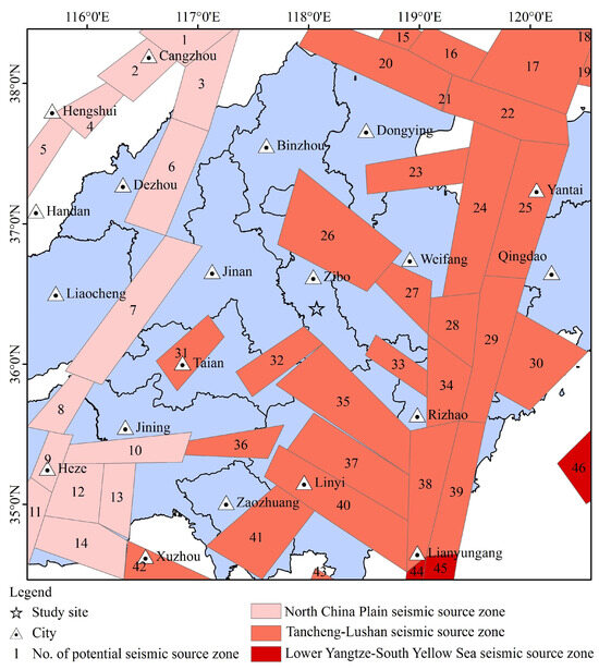
Figure 6.
Distribution of seismic zones and potential seismic source areas.
According to the fifth-generation seismic ground motion parameter zoning scheme, the values of M0, Mu, b and the annual average occurrence rate v4.0 for earthquakes above magnitude 4.0 in each seismic zone are shown in Table 6.
Table 6.
Seismic activity parameters.
There are 9 potential seismic source zones affecting the seismic hazard of the study area, and their seismic spatial distribution coefficients are shown in Table 7.
Table 7.
Seismic spatial distribution coefficients.
The fifth-generation seismic ground motion parameter zoning scheme specifies the PGA with a 10% probability of exceedance over 50 years as the design basis earthquake for general structures. Using the seismic safety assessment software SECR2019, the PGA values for the study site corresponding to 2%, 10% and 63% probabilities of exceedance over 50 years are calculated as 171.16 gal, 98.10 gal and 28.61 gal, respectively. These results place the study site within the 0.10 g zone, which corresponds to basic seismic intensity zone VII.
5. Seismic Fragility Assessment of the Study Object Based on the Monte Carlo Method and Response Surface Method
5.1. Uncertainty Analysis of Structural-Seismic Motion Samples
5.1.1. Probability Distribution and Normalization of Random Variables
In seismic analysis, uncertainties in bridge structures primarily arise from variations in material properties, geometric characteristics, and construction practices. Furthermore, ground motion intensity significantly influences structural responses [31]. Therefore, this study selected five random variables for fragility assessment: concrete elastic modulus Ec, damping ratio γ, steel yield strength fy, steel elastic modulus Es, and PGA. Among them, Ec, fy and Es follow log-normal distributions [32,33,34], whereas γ follows a normal distribution [35].
The Central Composite Design (CCD) method is a widely used approach for constructing response surface models due to its simplicity, efficiency, and reasonable number of required trials [36]. The random variables were normalized using the CCD method as shown in Equation (15). The probability distributions and corresponding statistical parameters of these random variables are summarized in Table 8.
where ξi, ξi,min and ξi,max denote the value, minimum value and maximum value of the i-th random variable, respectively; xi is the normalized value of the i-th random variable, where xi = 1, 0 and −1 represent ξi taking the maximum value, mean value and minimum value, respectively. i = 1, 2, 3, 4 and 5 represents the variables Ec, γ, fy, Es and PGA, respectively.
Table 8.
Probability distributions and statistical parameters of random variables.
5.1.2. Selection of Ground Motion Inputs
Due to the high lateral stiffness of the bridge, this study only considered longitudinal ground motion input. Fifteen measured ground motions were selected based on the target response spectrum, as listed in Table 9, with their acceleration response spectrum shown in Figure 7. These ground motions were carefully selected to be representative of the seismic hazard at the site, encompassing a range of magnitudes and source-to-site distances. The PGA of the measured ground motions was adjusted to 20 groups with intervals of 0.05 g, ranging from a minimum of 0 to a maximum of 1.0 g. The natural ground motions are amplitude-scaled to these values, resulting in a total of 300 ground motion records.
Table 9.
Measured ground motion information.
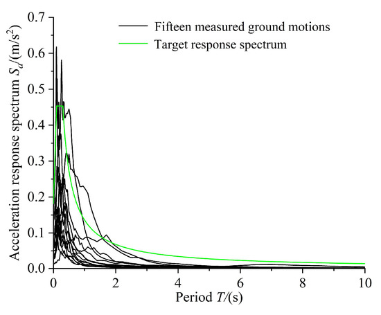
Figure 7.
Acceleration response spectrum.
5.2. Development of Response Surface Model
5.2.1. Introduction to Response Surface Model
The Response Surface Method is a statistical approach used to analyze the relationship between response variables and multiple input variables [37,38]. Owing to the nonlinear response of bridges under seismic action, a quadratic polynomial is typically selected as the response surface function [39,40], as expressed in Equation (16).
where k is the number of input variables, xi, and xj represent the values of input variables, a0, ai, aii and aij are undetermined coefficients estimated using the CCD method, and ε is the error term, which follows a normal distribution with a mean of zero.
For the finite element model of the bridge, conducting N = 2k + 2k + 1 times of IDA yields a system of linear equations for the unknow coefficients a0, ai, aii and aij. Using the least squares method to obtain the unbiased estimates of these undetermined coefficients, and validate the resulting response surface model using the coefficient of determination R2 and the adjusted coefficient of determination Ra2. Following common practice in response surface modeling, at least one of R2 and Ra2 is required to exceed 0.9 [41], as defined in Equations (17) and (18).
where α denotes the vector of undetermined coefficients, X represents the design matrix of variable, Y is the true response vector, E is the unit vector.
5.2.2. IDA Analysis Based on the CCD Method
This study selected k = 5, so the CCD method was used to design N = 43 groups of IDA. Each group comprised 15 ground records, yielding a total of 645 analyses. The mean values and standard deviations of the seismic damage parameters for the side piers, middle piers, and their corresponding bearings in each group were recorded, as summarized in Table 10.
Table 10.
Results of IDA.
The R2 and Ra2 values of the mean and standard deviation of the seismic damage parameters of the side piers, middle piers, and their corresponding bearings were calculated using Equations (17) and (18), as shown in Table 11.
Table 11.
Calculation results of R2 and Ra2.
From Table 11, both R2 and Ra2 exceed 0.9, confirming that the CCD method effectively captures trends in the simulation data and accurately reflects the influence of each random variable on the seismic damage of the bridge.
5.2.3. Solution of Response Surface Model
By integrating the data from Table 10 with Equation (16), the response surface model was solved. The response surface functions for the mean and standard deviation of the displacement ductility ratio ud of side piers are shown in Equation (19) and Equation (20), respectively.
The response surface functions for the mean and standard deviation of the displacement ductility ratio ud of middle piers are shown in Equation (21) and Equation (22), respectively.
The response surface functions for the mean and standard deviation of the shear deformation d of side pier bearings are shown in Equation (23) and Equation (24), respectively.
The response surface functions for the mean and standard deviation of the shear deformation d of middle pier bearings are shown in Equation (25) and Equation (26), respectively.
5.3. Plotting of Seismic Fragility Curves for the Research Object
5.3.1. Calculation of Seismic Exceedance Probability Based on Monte Carlo Method
Using the probability distributions of Ec, γ, fy and Es, 10,000 bridge samples were generated via the Monte Carlo Simulation. The PGA range was divided into 20 intensity levels from 0 to 1.0 g with an interval of 0.05 g. By inputting the 10,000 bridge samples across those 20 PGA levels through Equations (19) to (26), the corresponding seismic damage parameter values were obtained [42].
Combining Table 3 and Table 4, the number of bridge samples that reached and exceeded each seismic damage level under different PGA intensity levels, along with the corresponding exceedance probabilities were calculated using the method shown in Equation (27) [43].
where Pf denotes the exceedance probability of each level of seismic damage under different PGA intensity, where f = 1, 2, 3, 4 and 5 representing the intact, slight damage, moderate damage, severe damage and collapse states, respectively N(μ ≥ LSf), represents the number of bridge samples reaching or exceeding the f-th level of seismic damage.
The calculated exceedance probability for each seismic damage level of the bridge piers and pier bearings is shown in Table 12, Table 13, Table 14 and Table 15, respectively.
Table 12.
Exceedance probabilities of various seismic damage levels for side piers of the research object.
Table 13.
Exceedance probabilities of various seismic damage levels for middle piers of the research object.
Table 14.
Exceedance probabilities of various seismic damage levels for side pier bearings of the research object.
Table 15.
Exceedance probabilities of various seismic damage levels for middle pier bearings of the research object.
5.3.2. Seismic Fragility Curves of Bridge Piers
The seismic fragility curves of the side piers and middle piers were plotted, respectively, with the PGA on the horizontal axis and the exceedance probabilities of different seismic damage levels on the vertical axis, as shown in Figure 8 and Figure 9.
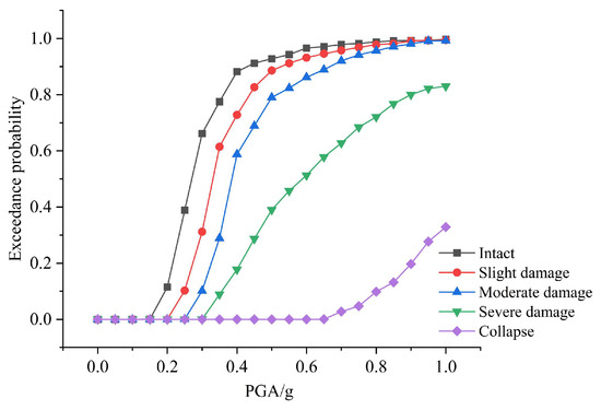
Figure 8.
Seismic fragility curves of side piers.
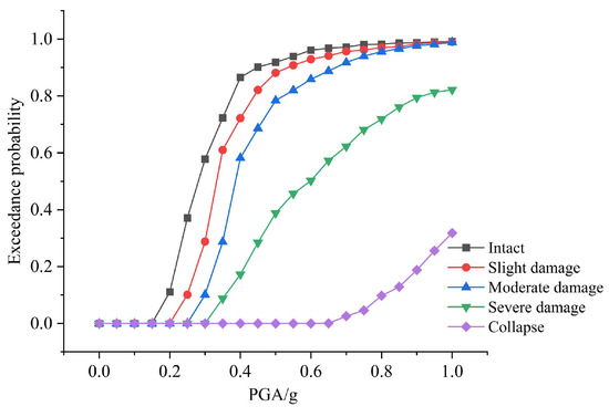
Figure 9.
Seismic fragility curves of middle piers.
From Figure 8 and Figure 9 show that as PGA increases, the exceedance probabilities of side piers and middle piers developing from intact state to collapse gradually rise, indicating a continuous increase in the fragility of bridge piers. At low PGA levels, the probability of slight damage is nearly zero, confirming minimal seismic effects on bridge piers. For slight and moderate damage states, the probability of damage increases rapidly until the PGA reaches approximately 0.3 g, beyond this value, the growth rate slows down and stabilizes. The fragility curves for slight and moderate damage are very close, which is attributed to the small difference in load-carrying capacity between these states, reflecting similar yield and equivalent yield curvatures in the pier reinforcement.
When the PGA gradually increases to about 0.5 g, severe damage begins to become distinctly apparent. The gap between the curves for moderate and severe damage indicates that the piers have a ductile behavior during this transition, which reduces the probability of severe damage and indicates a substantial difference between the curvature at equivalent yield and that at concrete crushing. Only when the PGA increases further do the piers begin to show complete collapse, and at the same PGA level, the exceedance probability of complete collapse is much lower than that of slight, moderate, or severe damage.
5.3.3. Seismic Fragility Curves of Bearings
Taking PGA as the horizontal axis and the exceedance probabilities of different seismic damage levels as the vertical axis, the seismic fragility curves for the side pier bearings and middle pier bearings of the research object were, respectively, plotted, as shown in Figure 10 and Figure 11.
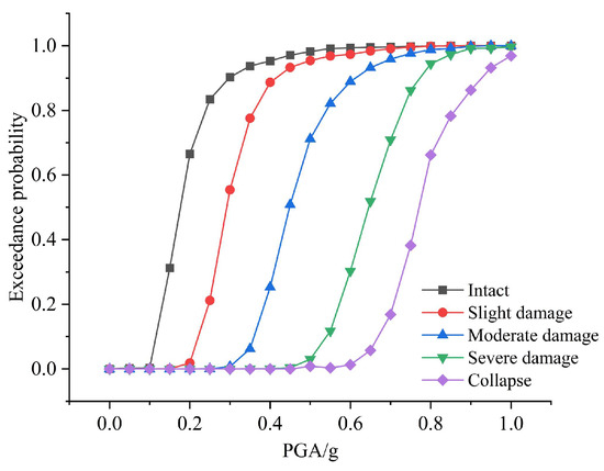
Figure 10.
Seismic fragility curves of side pier bearings.
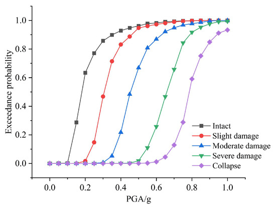
Figure 11.
Seismic fragility curves of middle pier bearings.
From Figure 10 and Figure 11, as PGA increase, the exceedance probabilities of bearings developing from an intact state to slight, moderate, severe damage, and collapse gradually rise, indicating growing fragility of bearings. At low PGA, the probability of slight damage is nearly zero, suggesting negligible seismic demands on the bearings. For slight and moderate damage, the probability of damage rises rapidly until the PGA reaches approximately 0.4 g; beyond which the rate increase slows and stabilizes. The fragility curves of slight and moderate damage lie close together, due to the small difference in load-carrying capacity between these damage states, indicating only minor changes in mechanical properties.
When the PGA increases to about 0.6 g, severe damage begins to appear. The notable separation between the moderate and severe damage curves, primarily the bearings, has a ductile behavior during this transition, which substantially reduces the probability of severe damage and indicates significant changes in mechanical properties between these damage stages. Only when the PGA further increases does the bearing exhibit collapse, and at the same PGA level, the exceedance probability of collapse is much lower than that of the other damage states.
5.4. Comparative Analysis and Methodological Enhancement
Conventional seismic fragility analyses often simplify or omit the explicit treatment of parametric uncertainties, which can lead to an incomplete assessment of structural fragility. For instance, the fragility assessment of RC frames by Abeysiriwardena et al. did not incorporate the uncertainties in key structural properties [12]. In contrast, the method proposed in this study provides a significant enhancement by systematically quantifying the coupled effects of uncertainties from four structural parameters and PGA. This is achieved by the integration of the Response Surface Method with large-scale Monte Carlo simulation, resulting in fragility curves that offer a more realistic and reliable representation of seismic performance, thereby establishing a more robust basis for risk assessment.
6. Seismic Probability Risk Assessment of the Research Object Based on Seismic Hazard Curve Method
6.1. Basic Theory
The seismic risk probability is mathematically defined as the convolution of seismic hazard and fragility, representing the integrated probability of exceeding each level of seismic damage under all seismic events over the next t years, as shown in Equation (28) [44].
where Pj,t is the risk probability of exceeding the j-th damage level over the next t years; Rj- represent the value of the seismic damage parameter corresponding to the j-th damage level; S is the value of the seismic damage parameter of the bridge under seismic action; xi is the PGA that the research site may encounter over the next t years. Due to the continuity of PGA values, Equation (28) can be rewritten as Equation (29).
where f(x) is the probability density function of PGA at the site over t years. The risk probability that the bridge will exceed the j-th level of seismic damage in the next 1 year as shown in Equation (30).
where H(x) is the annual distribution function of PGA at the site, whose shape is the seismic hazard curve, as shown in Equation (31) [45].
where k0 and k are parameters derived from the seismic hazard assessment results.
Based on the results of seismic fragility assessment, Equations (32) and (33) can be obtained.
where β is the dispersion parameter relating seismic damage to ground motion intensity; d1 and d2 are undetermined coefficients.
Equation (30) can be rewritten as Equation (34).
By performing integral transformation on Equation (34), Equation (35) can be obtained.
The standard normal cumulative distribution function yields Equation (36).
Then, Equation (35) can be further rewritten as Equation (37).
Simplifying Equation (37) yields Equation (38).
From Equation (33), Equation (39) is derived.
where PGAj- is the critical PGA corresponding to Rj-, substituting Equation (39) into Equation (38) gives Equation (40).
Referring to Equation (37), Equation (40) can be transformed into Equation (41).
6.2. Case Analysis
As shown in Table 12, Table 13, Table 14 and Table 15, under the same PGA levels, the seismic damage of the side piers is more severe than middle piers. Therefore, only the side piers and their bearings were considered in the probability risk assessment. According to the results of the IDA, for the bridge piers, the parameters are β = 0.8567, d1 = 1.082 and d2 = 0.995, for the bearings, the parameters are β = 0.8353, d1 = 76.853, and d2 = 0.99.
According to the results of seismic hazard assessment, the PGA values with different exceedance probabilities for the research site over the next 1 year are shown in Table 16.
Table 16.
PGA with different exceedance probabilities over 1 year.
Using Equation (31) and Table 16, the seismic hazard curve was plotted, as shown in Figure 12 and Equation (42).
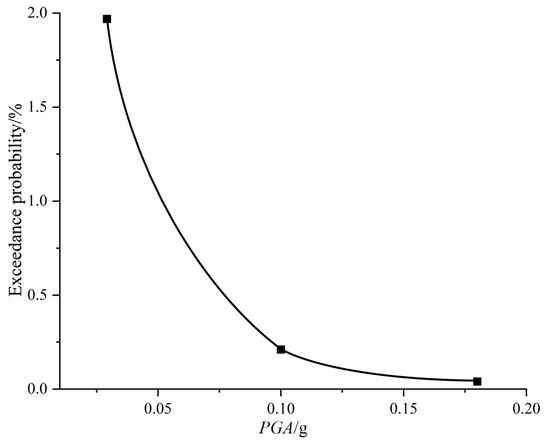
Figure 12.
Seismic hazard curve.
Using Equation (39) and Table 3 and Table 4, PGAj- was calculated, as shown in Table 17 and Table 18.
Table 17.
PGAj- corresponding to μd,max.
Table 18.
PGAj- corresponding to dmax.
Combining Equation (41) and (42), the risk probabilities of the bridge piers exceeding each level of seismic damage over 1 year are calculated as follows, slight damage P2,1 = 0.007424, moderate damage P3,1 = 0.005705, severe damage P4,1 = 0.001914 and collapse P5,1 = 0.000255. For the bearings, the probabilities are: slight damage P2,1 = 0.064627, moderate damage P3,1 = 0.014716, severe damage P4,1 = 0.006195 and collapse P5,1 = 0.004198.
Based on the Poisson distribution, a seismic occurrence probability prediction model is constructed. According to the assumptions of the Poisson distribution, it is considered that the probability of seismic events occurring each year and their impacts are independent of each other. The conversion method for the risk probabilities of the bridge piers and bearings exceeding each level of seismic damage over 1 year and over 50 years is shown in Equation (43).
Following calculations, the risk probabilities of the bridge piers and bearings exceeding each level of seismic damage over 50 years are shown in Table 19.
Table 19.
Assessment results of seismic damage risk probability for the research object.
7. Conclusions
This study systematically conducted seismic hazard, seismic fragility, and probability risk assessments using a reinforced concrete continuous girder bridge as a case study. First, the PGA with different exceedance probabilities at the study site was calculated using the CPSHA method from the fifth-generation seismic ground motion parameter zoning scheme. Second, the Monte Carlo method and Response Surface Method were integrated to characterize uncertainties in bridge structural parameters and PGA, and seismic fragility curves were plotted. Third, the risk probability was calculated based on the seismic hazard curve method, providing a theoretical basis for bridge seismic design and performance assessment. The research results were as follows.
(1) The study area is influenced by the Tancheng–Lushan, the Lower Yangtze–South Yellow Sea, and the North China Plain seismic source zones, involving a total of 46 potential seismic source zones. The PGAs with 2%, 10%, and 63% exceedance probabilities over the next 50 years at the site are 171.16 gal, 98.10 gal, and 28.61 gal, respectively, indicating that the site in the 0.10 g seismic intensity zone corresponds to basic intensity zone VII.
(2) As PGA increases, both side piers and middle piers show clear pattern of progression from an intact state to slight, moderate, severe, and eventually collapse. The exceedance probabilities for all levels of damage rise consistently with increasing PGA, strongly confirming that the intensity of ground motion is the core factor determining the extent of bridge pier damage. At the same PGA level, the exceedance probabilities for slight, moderate, severe, and collapse damage in side piers are generally higher than those in middle piers, confirming their higher seismic fragility. When the PGA is in the range of 0.4–0.6 g, the exceedance probability of moderate damage in side piers is significantly higher than that in middle piers, reflecting that side piers are more prone to moderate damage under moderate-intensity earthquakes. At high PGA levels (>0.8 g), the exceedance probability of collapse for side piers is also notably greater than for middle piers, indicating that side piers face a higher collapse risk. Based on these findings, seismic design for bridges should prioritize enhancing the seismic performance of side piers, using measures such as optimizing the structural configuration of side piers, strengthening anti-sliding and anti-fall beam measures at bearings, and reasonably installing seismic restraint devices to improve overall bridge seismic reliability.
Similarly, as PGA increases, both side and middle pier bearings exhibit progression from intact to slight, moderate, severe damage, and collapse, with the exceedance probabilities for all damage levels increasing with PGA. This fully demonstrates that ground motion intensity is the key factor affecting bearing damage. At the same PGA level, the exceedance probabilities for all damage levels in side pier bearings are generally higher than those in middle pier bearings, and their fragility curves lie above those of middle pier bearings. This indicates that side pier bearings are more susceptible to earthquake damage and show a more significant trend of damage escalation as PGA increases. In the range of 0.4–0.6 g, the exceedance probabilities of moderate damage for side pier bearings are significantly higher, and at PGA > 0.8 g, their collapse probabilities are also significantly greater.
(3) Over the next 50 years, the risk probabilities for the bridge piers to remain intact suffer slight, moderate, severe damage and collapse, at 68.90%, 6.22%, 15.75%, 7.86% and 1.27%, respectively. For the bearings, the corresponding probabilities are 3.54%, 44.11%, 25.64%, 7.74% and 18.97%, indicating that the overall seismic damage risk of bearings is higher than that of piers, especially for moderate damage and collapse. The high seismic risk of bearings necessitates targeted mitigation methods: (a) optimize design by adopting high-capacity isolation bearings and strengthening anti-unseating devices; (b) enhance inspection by incorporating bearings into routine and post-earthquake monitoring programs; and (c) promote retrofitting by installing external dampers or replacing conventional bearings with isolation or damping systems to improve overall resilience.
(4) The proposed seismic hazard–fragility–probability risk assessment system is applicable to various bridge structures and has high promotional and application value. While the specific risk probabilities are case-sensitive, the overall framework is generalizable to various bridge structures. Its application requires tailoring the finite element model and damage criteria to the specific structural system under investigation. However, there are still limitations: (a) omission of soil–structure interaction, potentially underestimate local risk; (b) lack of refined modeling bearing anchor bolts and stirrup spacing in plastic hinge regions, and unquantified impacts of construction quality variations; (c) only horizontal seismic motion input is used, ignoring multi-dimensional seismic motion effects on bearing shear deformation and pier flexural-shear failure; and (d) the validity of the finite element model relies on well-established modeling techniques rather than direct validation against experimental data from a physically identical bridge test. While the constitutive models and element formulations used have been extensively validated in the literature, future work should include a comprehensive experimental comparison to further corroborate the findings.
Author Contributions
Conceptualization, J.C.; Methodology, J.C. and C.Y.; Software, J.C. and C.Y.; Validation, J.C.; Resources, C.Y.; Data curation, J.C. and C.Y.; Writing – original draft, J.C.; Writing – review & editing, J.C., C.Y., T.S. and J.L.; Visualization, J.C.; Project administration, C.Y.; Funding acquisition, C.Y. All authors have read and agreed to the published version of the manuscript.
Funding
This research was supported by the National Natural Science Foundation of China (Grant No. 51808327) and the Natural Science Foundation of Shandong Province (Grant No. ZR2019PEE016).
Institutional Review Board Statement
Not applicable.
Informed Consent Statement
Not applicable.
Data Availability Statement
The data, models, and codes supporting the findings of this study are available from the corresponding author upon reasonable request.
Conflicts of Interest
The authors declare no conflict of interest.
References
- Han, Y.Y.; Zang, Y.; Meng, L.Y.; Wang, Y.; Deng, S.; Ma, Y.; Xie, M. A summary of seismic activities in and around China in 2021. Earthq. Res. Adv. 2022, 2, 100157. [Google Scholar] [CrossRef]
- Liu, J.L.; Jia, H.X.; Lin, J.Q.; Hu, H. Seismic Damage Rapid Assessment of Road Networks considering Individual Road Damage State and Reliability of Road Networks in Emergency Conditions. Adv. Civ. Eng. 2020, 2020, 9631804. [Google Scholar] [CrossRef]
- Ozsarac, V.; Monteiro, R.; Calvi, G.M. Probabilistic seismic assessment of reinforced concrete bridges using simulated records. Struct. Infrastruct. Eng. 2023, 19, 554–574. [Google Scholar] [CrossRef]
- Cornell, C.A. Engineering seismic risk analysis. Bull. Seismol. Soc. Am. 1968, 58, 1583–1606. [Google Scholar] [CrossRef]
- Pan, H.; Jin, Y.; Hu, Y.X. Discussion about the relationship between seismic belt and seismic statistical zone. Acta Seismol. Sin. 2003, 16, 323–329. [Google Scholar] [CrossRef]
- Bi, J.M.; Song, C.; Cao, F.Y. Declustering characteristics of the North China Plain seismic belt and its effect on probabilistic seismic hazard analysis. Sci. Rep. 2024, 14, 22170. [Google Scholar] [CrossRef] [PubMed]
- Vamvatsikos, D.; Cornell, C.A. Developing efficient scalar and vector intensity measures for IDA capacity estimation by incorporating elastic spectral shape information. Earthq. Eng. Struct. Dyn. 2005, 34, 1573–1600. [Google Scholar] [CrossRef]
- Wang, Q.A.; Wu, Z.Y.; Liu, S.K. Seismic fragility analysis of highway bridges considering multi dimensional performance limit state. Earthq. Eng. Eng. Vib. 2012, 11, 185–193. [Google Scholar] [CrossRef]
- Li, J.; Chen, J.B.; Sun, W.L.; Peng, Y.B. Advances of the probability density evolution method for nonlinear stochastic systems. Probabilistic Eng. Mech. 2012, 28, 132–142. [Google Scholar] [CrossRef]
- Yin, C.; Li, Y.; Liu, F.F. Probability risk assessment and management of embankment seismic damages based on CPSHA-PSDA. Iran. J. Sci. Technol. Trans. A Sci. 2019, 43, 1563–1574. [Google Scholar] [CrossRef]
- Che, F.; Yin, C.; Zhang, H.; Tang, G.T.; Hu, Z.N.; Liu, D.; Li, Y.; Huang, Z.F. Assessing the risk probability of the embankment seismic damage using Monte Carlo method. Adv. Civ. Eng. 2020, 2020, 8839400. [Google Scholar] [CrossRef]
- Abeysiriwardena, T.M.; Wijesundara, K.K.; Nascimbene, R. Seismic risk assessment of typical reinforced concrete frame school buildings in Sri Lanka. Buildings 2023, 13, 2662. [Google Scholar] [CrossRef]
- Cheng, X.L.; Li, Q.Q.; Hai, R.; He, X.F. Study on seismic vulnerability analysis of the interaction system between saturated soft soil and subway station structures. Sci. Rep. 2023, 13, 7410. [Google Scholar] [CrossRef] [PubMed]
- Zhou, X.H.; Zhou, Z.; Gan, D. Modeling of cyclically loaded square thin-walled CSFT columns stiffened by diagonal ribs using OpenSees. Thin-Walled Struct. 2023, 187, 110736. [Google Scholar] [CrossRef]
- Tatar, A.; Baker, A.M.; Dowden, D.M. A generalized method for numerical modeling of seismically resilient friction dampers using flat slider bearing element. Eng. Struct. 2023, 275, 115248. [Google Scholar] [CrossRef]
- Guan, M.S.; Hang, X.R.; Wang, M.S.; Zhao, H.Y.; Liang, Q.Q.; Wang, Y. Development and implementation of shear wall finite element in OpenSees. Eng. Struct. 2024, 304, 117639. [Google Scholar] [CrossRef]
- GB/T 24335-2009; Classification of Earthquake Damage to Buildings and Special Structures. National Technical Committee for Seismological Standardization: Beijing, China, 2009.
- Bhatta, S.; Dang, J. Seismic damage prediction of RC buildings using machine learning. Earthq. Eng. Struct. Dyn. 2023, 52, 3504–3527. [Google Scholar] [CrossRef]
- Yamaguchi, T.; Mizutani, T. A Physics-Informed Neural Network for the Nonlinear Damage Identification in a Reinforced Concrete Bridge Pier Using Seismic Responses. Struct. Control Health Monit. 2024, 2024, 5532909. [Google Scholar] [CrossRef]
- Qiu, W.H.; Wang, K.H.; Guo, W.Z. Seismic Performance of the Wall Pier of Covered Bridge in the Weak Direction. Iran. J. Sci. Technol. Trans. Civ. Eng. 2024, 48, 4183–4200. [Google Scholar] [CrossRef]
- Song, S.; Qian, Y.J.; Liu, J.; Xie, X.R.; Wu, G. Time-variant fragility analysis of the bridge system considering time-varying dependence among typical component seismic demands. Earthq. Eng. Eng. Vib. 2019, 18, 363–377. [Google Scholar] [CrossRef]
- Zhong, H.Q.; Yuan, W.C.; Dang, X.Z.; Deng, X.W. Seismic performance of composite rubber bearings for highway bridges: Bearing test and numerical parametric study. Eng. Struct. 2022, 253, 113680. [Google Scholar] [CrossRef]
- Xu, W.J.; Wu, J.; Gao, M.T. Seismic hazard analysis of China’s mainland based on a new seismicity model. Int. J. Disaster Risk Sci. 2023, 14, 280–297. [Google Scholar] [CrossRef]
- Iwata, D.; Nanjo, K.Z. Adaptive estimation of the Gutenberg–Richter b value using a state space model and particle filtering. Sci. Rep. 2024, 14, 4630. [Google Scholar] [CrossRef] [PubMed]
- Cao, X.Y.; Feng, D.C.; Beer, M. Consistent seismic hazard and fragility analysis considering combined capacity-demand uncertainties via probability density evolution method. Struct. Saf. 2023, 103, 102330. [Google Scholar] [CrossRef]
- Pei, W.L.; Zhou, S.Y.; Zhuang, J.C.; Xiong, Z.Y.; Piao, J. Application and discussion of statistical seismology in probabilistic seismic hazard assessment studies. Sci. China (Earth Sci.) 2022, 65, 257–268. [Google Scholar] [CrossRef]
- Han, S.C.; Sun, J.Z.; Xiong, F. Analysis for site seismic hazard probability considering the orientation distribution of potential seismic sources. Nat. Hazards 2024, 121, 2433–2464. [Google Scholar] [CrossRef]
- Vandana; Dadhich, H.K.; Mittal, H.; Mishra, O.P. Ground motion prediction equation for NW Himalaya and its surrounding region. Quat. Sci. Adv. 2024, 13, 100136. [Google Scholar] [CrossRef]
- Eskandarinejad, A.; Shiau, J.; Keawsawasvong, S. Effect of Depth-Dependent Shear Wave Velocity Profiles on Site Amplification. Transp. Infrastruct. Geotechnol. 2022, 10, 1255–1283. [Google Scholar] [CrossRef]
- Zhong, Z.L.; Shen, Y.Y.; Zhao, M.; Li, L.Y.; Du, X.L. Seismic performance evaluation of two-story and three-span subway station in different engineering sites. J. Earthq. Eng. 2022, 26, 7505–7535. [Google Scholar] [CrossRef]
- Yin, K.S.; Xu, Y.; Li, J.Z.; Zhou, X. Gaussian process regression driven rapid life-cycle based seismic fragility and risk assessment of laminated rubber bearings supported highway bridges subjected to multiple uncertainty sources. Eng. Struct. 2024, 316, 118615. [Google Scholar] [CrossRef]
- Liu, Y.Y.; Chen, J.B.; Li, J. The modified mesoscopic stochastic fracture model incorporating the random field of Young’s modulus for the uniaxial constitutive law of concrete. Probabilistic Eng. Mech. 2024, 75, 103585. [Google Scholar] [CrossRef]
- Chen, Y.X.; Zhang, J.Y.; Ma, J.C.; Zhou, S.L.; Liu, Y.S.; Zheng, Z.X. Tensile strength and fracture toughness of steel fiber reinforced concrete measured from small notched beams. Case Stud. Constr. Mater. 2022, 17, e01401. [Google Scholar] [CrossRef]
- Ge, F.W.; Tong, M.N.; Zhao, Y.G. A structural demand model for seismic fragility analysis based on three-parameter lognormal distribution. Soil Dyn. Earthq. Eng. 2021, 147, 106770. [Google Scholar] [CrossRef]
- Hu, X.N.; Fang, G.S.; Ge, Y.J. Uncertainty propagation of flutter derivatives and structural damping in buffeting fragility analysis of long-span bridges using surrogate models. Struct. Saf. 2024, 106, 102410. [Google Scholar] [CrossRef]
- Xiang, Z.; Zhu, Z.W. Multi-objective optimization of a composite orthotropic bridge with RSM and NSGA-II algorithm. J. Constr. Steel Res. 2022, 188, 106938. [Google Scholar] [CrossRef]
- Sun, D.L.; Wang, J.; Wen, H.J.; Ding, Y.K.; Mi, C.L. Landslide susceptibility mapping (LSM) based on different boosting and hyperparameter optimization algorithms: A case of Wanzhou District, China. J. Rock Mech. Geotech. Eng. 2024, 16, 3221–3232. [Google Scholar] [CrossRef]
- Kong, D.H.; Luo, Q.; Zhang, W.S.; Jiang, L.W.; Zhang, L. Reliability analysis approach for railway embankment slopes using response surface method based Monte Carlo simulation. Geotech. Geol. Eng. 2022, 40, 4529–4538. [Google Scholar] [CrossRef]
- Pang, Y.T.; Meng, R.; Li, C.D.; Li, C. A probabilistic approach for performance-based assessment of highway bridges under post-earthquake induced landslides. Soil Dyn. Earthq. Eng. 2022, 155, 107207. [Google Scholar] [CrossRef]
- Liu, Y.; Meng, X.L.; Hu, L.L.; Bao, Y.; Hancock, C. Application of Response Surface-Corrected Finite Element Model and Bayesian Neural Networks to Predict the Dynamic Response of Forth Road Bridges under Strong Winds. Sensors 2024, 24, 2091. [Google Scholar] [CrossRef]
- Huang, J.; Qiu, S.Q.; Rodrigue, D. Parameters estimation and fatigue life prediction of sisal fibre reinforced foam concrete. J. Mater. Res. Technol. 2022, 20, 381–396. [Google Scholar] [CrossRef]
- Cabanzo, C.; Mendes, N.; Akiyama, M.; Lourenço, P.B.; Matos, J.C. Probabilistic framework for seismic performance assessment of a multi-span masonry arch bridge employing surrogate modeling techniques. Eng. Struct. 2025, 325, 119399. [Google Scholar] [CrossRef]
- Ashrafifar, J.; Estekanchi, H. Life-cycle seismic fragility and resilience assessment of aging bridges using the endurance time method. Soil Dyn. Earthq. Eng. 2023, 164, 107524. [Google Scholar] [CrossRef]
- Li, S.Q.; Gardoni, P. Seismic loss assessment for regional building portfolios considering empirical seismic vulnerability functions. Bull. Earthq. Eng. 2024, 22, 487–517. [Google Scholar] [CrossRef]
- Kan, C.Y.; Tsai, C.C.; Chen, C.J. Simple method for probabilistic seismic landslide hazard analysis based on seismic hazard curve and incorporating uncertainty of strength parameters. Eng. Geol. 2023, 314, 107002. [Google Scholar] [CrossRef]
Disclaimer/Publisher’s Note: The statements, opinions and data contained in all publications are solely those of the individual author(s) and contributor(s) and not of MDPI and/or the editor(s). MDPI and/or the editor(s) disclaim responsibility for any injury to people or property resulting from any ideas, methods, instructions or products referred to in the content. |
© 2025 by the authors. Licensee MDPI, Basel, Switzerland. This article is an open access article distributed under the terms and conditions of the Creative Commons Attribution (CC BY) license (https://creativecommons.org/licenses/by/4.0/).