Abstract
Affected by the improper operation of the workers, environmental changes during drying and curing or the quality of the paint itself, diverse defects are produced during the process of ship painting. The traditional defect recognition method relies on expert knowledge or experience to detect defects, which is not conducive to ensuring the effectiveness of defect recognition. Therefore, this paper proposes an image generation and recognition model which is suitable for small samples. Based on a deep convolutional neural network (DCNN), the model combines a conditional variational autoencoder (DCCVAE) and auxiliary conditional Wasserstein GAN with gradient penalty (ACWGAN-GP) to gradually expand and generate various coating defect images for solving the overfitting problem due to unbalanced data. The DCNN model is trained based on newly generated image data and original image data so as to build a coating defect image classification model suitable for small samples, which is conducive to improving classification performance. The experimental results showed that our proposed model can achieve up to 92.54% accuracy, an F-score of 88.33%, and a G mean value of 91.93%. Compared with traditional data enhancement methods and classification algorithms, our proposed model can identify various defects in the ship painting process more accurately and consistently, which can provide effective theoretical and technical support for ship painting defect detection and has significant engineering research value and application prospects.
1. Introduction
The shipbuilding industry is an indispensable and important part of the national equipment manufacturing industry, is the epitome of modernized industry, and is also a strategic industry related to national economic development and national defense. As one of the three pillars of modern shipbuilding process, ship painting runs through the whole process of shipbuilding, from design and construction to the delivery of the ship [1,2]. Coating quality is directly related to the construction cycle and maintenance cost of the ship as well as an important factor affecting the corrosion resistance of the hull and the service life of the ship [3]. Without modern ship painting, there is no modern shipbuilding. However, in the process of ship painting, various defects such as holiday coating, sagging and orange skin are produced due to worker error and environmental changes during drying and curing [4]. These coating defects not only affect the aesthetic appearance, but also have an impact on the performance of the coating, which in turn leads to severe corrosion of the hull surface [5]. Therefore, in the field of ship construction, timely identification of coating defects and feedback regarding the painting process is essential to improve the quality of ship construction and enhance the core competitiveness of ship enterprises.
Feature extraction is to extract effective feature information from images, which is usually used as a basis for image classification [6,7,8]. Conventional coating defect detection is the inspection and judging of coating quality and the recording of the type and level of defects the staff produces within a specific time after the painting is completed. This method relies on domain experts or field technicians to identify the underlying visual features of defects, such as color [9,10,11,12], shape [13,14,15,16], and texture [17,18,19,20] through professional knowledge and practical experience, which not only increases the work intensity and work pressure of personnel but also greatly increases time cost, making it difficult to ensure the accuracy of coating defect identification [21] and the efficiency of coating operations [22]. With proposals based in ship manufacturing theory and the continuous popularization of artificial intelligence in the ship painting industry, people have begun to gradually apply intelligent technology to the understanding of ship painting defects, but there are fewer reports on the application of image-based ship coating defects recognition.
The deep learning theory represented by convolutional neural networking can simulate the function of the visual center of the human brain and automatically extract deeper features from information without artificially designing feature patterns, which can truly achieve “end-to-end” recognition [23] and, to a certain extent, solve the problem that traditional machine learning methods [24] cannot classify high-dimensional data [25] and the classification process requires professional knowledge and complex computing power [26]. Since its introduction, it has received a lot of attention from scholars and has achieved great success in computer vision [27], natural language processing [28], image processing [29] and other fields. However, in practical applications, due to various reasons such as high labeling cost, severe natural image noise, data security and privacy protection, there is no special and large number of labeled ship coating defect datasets available for the training of deep learning network models and numerous hyper-parameter adjustments. Based on the above reasons, it is difficult to obtain a sufficient and balanced dataset from the existing ship coating defect image classification. Therefore, the data-driven deep learning model faces the problem of data imbalance, which limits the reliability of the model. Analysis shows that the classification model with a dimensionality approximation equal to or greater than the sample size of the original feature space may have several problems such as overfitting [30] and poor generalization performance [31], which restricts the development of a new generation of artificial intelligence seriously.
Researchers both at home and abroad have conducted a lot of research on the few-shot problem. Liu Jinxiang et al. [32] combined the multidimensional convolution layer with the attention mechanism module to solve the few-shot problem in hyperspectral image classification. Dong Yunjia [33] used the bearing dynamics model to generate massive and diverse simulation data, and, combined with transfer learning, the network can learn more transferable features, reduce the difference of feature distribution, and significantly improve the fault recognition performance of rolling bearings. Hongmin Gao et al. [34] constructed a small convolution and feature taking module, which can extract the spectral and spatial features of HIS at the same time even in the case of limited training samples, effectively improving the generalization ability of CNN. The above results have laid a good theoretical foundation for the research on this subject. However, at present, in the field of shipbuilding, especially in the field of coating defect recognition, the imbalance of sample categories is still an important factor restricting the performance of defect detection [35]. Due to the unbalanced ship coating defect data, the traditional trained classification model cannot easily identify certain classes, which results in an over-fitting model and its overall generalization performance is greatly reduced.
In general, data augmentation methods can be used to solve the above problems [36]. Traditional data augmentation methods such as geometric transformations, color transformations and pixel transformations [37] focus on generating image data via simple linear transformations, which preserve labels only by simply modifying the image to merge affinities without producing completely invisible data [38]. It can be seen that these traditional data enhancement methods can only expand the number of images through depth and scale in the process of image classification, which has no practical utility for clearly distinguishing data boundaries, although it alleviates the data imbalance problem to some extent [39]. This type of data augmentation does not improve the data distribution determined by higher-level features and thus cannot change the sample categories [40,41]; therefore, these traditional data augmentation methods have no practical utility in recognizing minority categories. A modern and advanced form of data enhancement is synthetic data enhancement, which overcomes the limitations of traditional data enhancement. Variational autoencoders (VAEs) and generative adversarial networks (GANs) are two of the most popular deep generative models [42] and are widely used in areas such as image generation [43], image transformation [44], image resolution enhancement [45], domain adaptation [46] and anomaly detection [47]. Ngoc-Trung Tran et al. [48] proposed a GAN-based data enhancement optimization model and validated the proposed GAN model to obtain better FID performance on natural and medical datasets; Santiago López-Tapia et al. [49] extended image super-resolution to video super-resolution, demonstrating that the proposed system obtained higher super-resolution than the perceptual quality provided by the MSE-based model; Jang Young In et al. [50] generated simulated ECG signals by variational self-encoder (VAE) reconstruction to enhance the consistency of SDNN. However, recent studies have shown that although the original GAN has many advantages when applied, it still suffers from non-convergence, gradient vanishing, difficulty in generating controllable multi-class and high-quality datasets [51], unstable training process [52], single input noise [53] and mode collapse [54], due to the fact that GANs involve unsupervised learning. Like GANs, VAEs, which serve as new sample generation models, can reconstruct images by inputting random noise and thus by variational inference [55] optimization methods. However, they are not able to reconstruct the target image through adversarial learning mechanisms like GANs can. Moreover, the images generated by VAE reconstruction are often blurred due to the lack of perfect optimization measurements and unavoidable noise due to manually designed parameters. Therefore, it has become urgent to combine the advantages of both models to compensate for the inherent weaknesses of each.
To address the above situation, this paper proposes an image generation and recognition algorithm model for small samples, which combines the sample generation capability of conditional variational autoencoder (CVAE) and the adversarial learning mechanism of GANs based on DCNNs, extends and generates a variety of coating defective images and trains the DCNN model together with the original images to improve classification performance, effectively solving the problems of overfitting caused by small samples and model collapse caused by data imbalance. The contributions of this paper are summarized as follows:
- At present, the transformation and upgrading of the shipbuilding industry driven by intelligent manufacturing is in its infancy. Aimed at the problems of over-reliance on domain expert knowledge and low intelligence level in the current stage of ship coating defect recognition, this paper proposes an intelligent coating defect recognition algorithm. Based on the data enhancement network model, painting defect images are generated, and the “end-to-end” recognition model is trained.
- Traditional data augment methods cannot change the sample categories. To solve this problem, this paper first combines the ideas of DCCVAE and ACWGAN-GP at the data level, so that the network can generate high-quality, multi-category images of minor ship coating defects in accordance with the original data distribution in a more stable and controllable way.
- The standard DCCVAE encoding stage is not conducive to feature extraction by establishing a connection with class labels instead. To solve this problem, this paper only adds class labels in the decoding stage.
- To avoid the problems of gradient disappearance and model overfitting inherent in the deep generation model, this paper introduces the residual block with an attention mechanism to fully extract the important features. At the same time, the algorithm model loss function is improved from the algorithm level to prevent problems such as gradient disappearance and gradient explosion to some extent. Then, the balanced dataset is used as the input of DCNN deep neural network, and the parameters are globally tuned by “layer-by-layer pre-training + fine-tuning” to obtain the optimal DCNN model parameters. Finally, the trained DCNN neural network is used to classify the coating defects in the test set, and the final classification results are obtained.
The results show that the proposed method is better than other data enhancement algorithms in achieving high accuracy detection and identification of ship coating defects under small sample conditions.
2. Proposed Methodology
2.1. The Overall Framework of the Proposed Model
The proposed classification algorithm for ship coating defects consists of four modules, namely a data acquisition module, a data pre-processing module, a data generation module and a coating defect classification module, as shown in Figure 1.
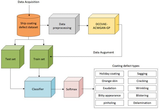
Figure 1.
The framework of the proposed image classification method for ship coating defects.
Based on the above framework, the DCCVAE-ACWGAN-GP model is chosen as the model of the data generation module in this paper, which consists of four sub-networks with a convolutional neural network as the main architecture, that is, an encoder network (En), decoder network (De), generator network (G) and discriminator network (Dis), as shown in the module (F) in Figure 2. The detailed flowchart of the proposed algorithm model is as follows. The upper half of the dotted line of the module (F) is the training process of ACWGAN-GP, and the lower half is the training process of DCCVAE.
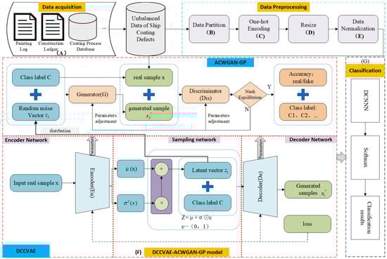
Figure 2.
Specific recognition process of ship coating defect images based on DCCVAE-ACWGAN-GP.
STEP1: Data acquisition (A): The unbalanced coating defect database is collected through painting logs, construction ledgers and a painting process database in the shipyard.
STEP2: Data pre-processing: This mainly consists of four stages, namely, data partition (B), one-hot encoding (C), resizing (D) and data normalization (E). The specific steps are as follows.
STEP2.1: Data partition (B): The original database obtained in STEP1 is divided into a training set, a testing set and a validation set at a ratio of 0.7:0.15:0.15.
STEP2.2: One-hot encoding (C): The class labels of 10 coating defect images converted to one-hot encoding are concatenated with random noise vector z, to serve as the input to the decoder De. For example, the label of Holiday coating is one-hot encoded as [1,0,0,0,0,0,0,0,0,0] and the label of Sagging as [0,1,0,0,0,0,0,0,0,0].
STEP2.3: Resize (D): Since the size ratio of the acquired images varies in the coating defect dataset, all images are resized to 128 × 128 × 3.
STEP2.4: Data normalization (E): Since large differences in values tend to lead to slow convergence of the network and saturation of neuron outputs, each image is normalized by rescaling the pixels from [0,255] to [0,1] (data normalization is a process of changing the range of pixel values, the purpose of which is to transform the input image into a series of more familiar or normal pixel values, ensuring that each feature is in the same dimension and greatly improving the performance of the neural network).
STEP3: Coating defect image generation based on DCCVAE-ACWGAN-GP model: This consists of two phases, namely the DCCVAE model training phase and the ACWGAN-GP model training phase.
STEP3.1: DCCVAE model training phase: Input real sample x without labels to the encoder of DCCVAE after data preprocessing to obtain a latent distribution with mean µ and standard deviation , and then the latent representation z is sampled from the distribution by the reparameterization trick (), and the newly generated samples are obtained from the learned distribution by the decoder De.
STEP3.2: ACWGAN-GP model training phase: After the training of the DCCVAE is completed, since the DCCVAE and ACWGAN-GP have the same architecture, we use the network parameters pre-trained by the DCCVAE to initialize the network parameters in the ACWGAN-GP, which improves the training efficiency of the ACWGAN-GP and also minimizes the differences of training. In addition, due to the difficulty of noise sampling, this paper uses the prior distribution learned by the DCCVAE for random noise sampling to obtain the noise vector. Together with the category label C as the input of the generator in ACWGAN-GP, we obtain the specific generation samples . Then the discriminator keeps the distance to destroy the real image and the generated image to form the training process of confrontation and generate the classification prediction.
STEP4: a coating defect classification using the DCNN model: The newly generated coating defect images are first blended into the original dataset to form a new balanced dataset. Then, the newly generated images are used as the input to train the DCNN model. Additionally, the network parameters are updated and optimized through iteration and fine-tuning and output the classification results through the trained classifier. The final classification results are tested and validated on the original dataset.
2.2. The Training Process and Total Loss Function of the Proposed Model
2.2.1. The Training Process of the Proposed Algorithm
The training process of the DCCVAE-ACWGAN-GP algorithm model, as shown in Algorithm 1.
| Algorithm 1: Training process of DCCVAE-ACWGAN-GP model |
| Input: batch size m, number of categories n, learning rate α, number of iteration k, spatial dimension of the noise z Output: Initialize network parameters of different networks While i < the maximum number of iterations or model parameters converges do 1: ← mini-batch sampling randomly from the real coating defect data set For each real minority sample do 2: Obtain the feature parameter vector µ, σ ← input x to the Encoder network 3: Obtain the potential representation ← re-parameterization trick () 4: Generate specific samples ← reconstruct by the Decoder network 5: Feed real samples and generated samples into discriminator network Dis to distinguish true from false 6: Feed real samples and generated samples into the Classification network C to ensure the recognition of coating defect categories and the final classification results are tested and verified in the original dataset. 7: Optimize the loss function of DCCVAE-ACWGAN-GP model: sampling from the initial distribution N(0,1) ← obtain ς by random sampling from a Gaussian distribution 8: Update network parameters: End For End While Print(New structure) End |
2.2.2. Loss Function
The goal of the proposed model is to minimize the loss function, which has four components, as shown in Equation (1).
where and is the Kullback–Leibler divergence and the reconstruction loss in DCCVAE model, as shown in Equation (2) and Equation (3), respectively.
where k is the dimension of the latent variable z. Since the dimension of the potential vector z in this paper is 100 × 1, k is 100.
is the loss function of the ACWGAN-GP model, which consists of three parts: generator loss , discriminator loss and gradient penalty (GP), as shown in Equation (4), Equation (5) and Equation (6), respectively.
where is the gradient of the discriminator network Dis, and represents the Euclidean norm of the discriminator network Dis gradient.
Therefore, the final loss function of the ACWGAN-GP model is shown in Equation (7).
where ϒ is the weight coefficient of the ACWGAN-GP gradient penalty.
is the loss function of the classification network DCNN, as shown in Equation (8).
In summary, the total loss function of the proposed model is shown in Equation (9).
where β, ψ and λ are the weight parameters that adjust the loss function of each sub-network to maintain balance between the individual loss functions.
2.3. The Structure Design of the Proposed Model
2.3.1. The Structure of the DCCVAE Network Model
In this study, we propose a DCCVAE model to generate images for each defect, but with a different structure from the standard CVAE network. First of all, the conditional probability distributions of both the encoder and decoder of the standard CVAE are related to the label C. There is no need to link the features to the category labels in the coating defect recognition task, so in this paper, we only add the class label C in the decoding stage, which is more beneficial to feature extraction in the encoding stage. Secondly, when the deep network reaches a certain depth, increasing the number of layers blindly does not further improve the classification performance. On the contrary, it will make the network more difficult to train. Therefore, in order to fully extract important features and avoid the problems of gradient disappearance and model overfitting due to the deepening of network layers, we introduce residual blocks with attention mechanisms to improve the generalization ability of the network. The detailed description of the proposed DCCVAE network model structure is shown in Figure 3. Also, the detailed network parameters of the encoder and decoder in DCCVAE are shown in Table 1 and Table 2, respectively.
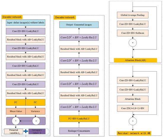
Figure 3.
The detailed description of the proposed DCCVAE network model structure.

Table 1.
The detailed network parameters of the encoder in DCCVAE model.
Table 2.
The detailed network parameters of the decoder in DCCVAE model.
- Encoder network
As shown in Table 1, in the proposed encoder, we implement one input layer, four basic convolutional blocks, two fully connected layers and one output layer. Each convolutional block consists of one convolutional layer with 3 × 3 filters and 2 × 2 strides, followed by BN, a LeakyReLU activation function. In addition, a residual block with an attention block is added after each convolutional block of the encoder, which contains three convolutional layers with 3 × 3 kernels.
- 2.
- Decoder network
The decoding process is the reverse operation of the encoding process. To ensure that the size of the generated image is the same as the size of the original input, the decoder uses a symmetric structure similar to that of the encoder. We use transposed convolutional layers to implement spatial upsampling instead of convolutional layers. Similar to the encoder network, the decoder consists of one FC+BN+LeakyReLU layer, four convolutional blocks and one output layer, as shown in Figure 4. We use one fully connected layer in the potential vector to extend the dimension. Then an 8 × 8 × 1024 feature map is generated. In addition, we place 4 transposed convolution blocks consisting of a 3 × 3 filter to increase the size, a batch normalization (BN) layer and a LeakyReLU activation layer with a slope of 0.2.
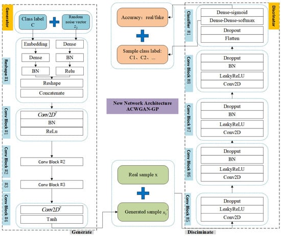
Figure 4.
The detailed description of the proposed ACWGANGP network model structure.
Like the encoder, each transposed convolutional layer is followed by a residual block with an attention mechanism. The differences are as follows: first, a residual block is added after each transposed convolutional layer except the last one. Second, we choose the Sigmoid function as the activation function of the output layer of the decoder. The detailed decoder structure is shown in Table 2.
2.3.2. The Structure of the ACWGAN-GP Network Model
The ACWGAN-GP model proposed in the paper is one of the standard GAN variants. It inherits the conditional image generation of ACGAN and the training stability of WGAN-GP to make up for the inherent deficiencies of their respective models, as shown in Figure 4. Compared with other GANs, the ACWGAN-GP model proposed in this paper can both generate images with class-specific labels and use Wasserstein distance instead of Jensen–Shannon (JS) divergence to evaluate the distribution differences between real and generated samples, which alleviates the gradient disappearance and model collapse problems associated with overtraining of GANs models. In addition, a Wasserstein GAN with gradient penalty (WGAN-GP) is chosen instead of weight clipping to limit the gradient parametric update range of the objective function to no more than 1 without extensive hyperparameter tuning, to prevent gradient explosion and to use gradient penalty measurements to satisfy the Lipschitz constraint. This makes WGAN models faster to train, and the training process more stable. In this work, we use a CNN as the main architecture of the generator and discriminator. Details of the model architecture are shown in Table 3 and Table 4. Part of the image generated by the model is shown in Figure 5.
Table 3.
The detailed network parameters of the generator in ACWGAN-GP model.
Table 4.
The detailed network parameters of the discriminator in the ACWGAN-GP model.
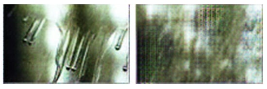
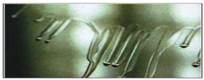
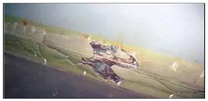
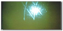
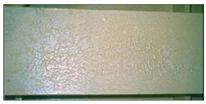
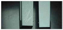
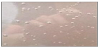
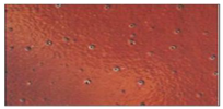
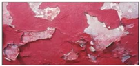
Figure 5.
The following is the sagging image generated by the ACWGAN-GP model.
- Generator model
Similar to DCCVAE, the generator consists of one reshape layer and four deconvolution blocks. As shown in Figure 4, the first three deconvolution blocks contain one deconvolution layer with a 3 × 3 kernel and a stride size of 2, a BN layer and a ReLU activation layer among them. The last deconvolution block uses Tanh as the output activation function. To avoid the problem of overfitting, the BN layer, as a regularization technique, is used after each convolutional layer in the proposed architecture. The detailed network parameters of the generator are shown in Table 3.
- 2.
- Discriminator network
Similar to the generator, the proposed discriminator also consists of four convolutional blocks and one classification layer. Among them, each convolutional block consists of 1 convolutional layer with a convolutional kernel of 3 × 3 and a stride size of 2, followed by a LeakyReLU activation layer, a BN layer and a dropout layer with a dropout rate of 0.5. In the classification layer, it is necessary to add a dense layer at the end of the network in order to classify the features generated by the convolutional layer. Finally, the result is output after the addition of two fully connected layers. One of the fully connected layers outputs the probability of the image being true using the Sigmoid function and the other outputs the corresponding probabilities of the 10 coating defect classes using the Softmax function. The detailed network parameters of the discriminator are shown in Table 4.
2.3.3. The Structure of the Classification Network Model
Conv2D layers and pooling layers are more suitable for filtering the spatial localization of painted defective images. Therefore, we propose a convolutional layout-based classification network that can classify painting defects using the training data generated by the DCCVAE-ACWGAN-GP. The architecture of the model is shown in Figure 6.
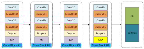
Figure 6.
The detailed description of the proposed DCNN model structure.
As shown in Figure 6, the classification network consists of four convolutional blocks and one classification layer with a sliding window of 2. Each convolutional block contains a Conv2D layer with a 3 × 3 kernel, a LeakyReLU activation layer with a slope of 0.2 and a dropout layer with a dropout rate of 0.5. The first three convolutional blocks use a 2 × 2 max-pooling layer, except for the fourth convolutional block which uses a global average pooling (GAP) layer. The classifier consists of one fully connected layer. The final activation function uses a Softmax function to output a probability value between 0 and 1, which reduces the number of training parameters and improves the classification performance. The detailed structure of the classification model is shown in Table 5.
Table 5.
The detailed network parameters of the DCNN model.
2.4. The Training Process Optimization Strategies and Implementation Details
Based on the above loss functions, we use the RMSProp optimizer for stochastic gradient descent optimization of the model parameters because the discriminant loss is unstable, and momentum-based optimization algorithms, such as Adam’s algorithm, perform worse, while the RMSProp optimizer performs well even in very unstable cases. To improve the stability of ACWGAN, the learning rates of the generator G and the discriminator Dis are unequal. Similar to the GAN framework, the discriminator D parameters are updated k times, and then the G parameters are updated once. In order to prevent the generator and discriminator training process from being inconsistent and leading to a fixed loss value of the generator and the gradient explosion problem, the discriminator is usually updated once and the generator is updated k times (k is greater than 1), and in this paper, the learning rate of generator G is 0.0003, while the learning rate of discriminator Dis is 0.0001, and the parameters are updated iteratively, as shown in Table 6.
Table 6.
The parameters configuration of the proposed network model.
3. Experiments Setup and Results
3.1. Dataset
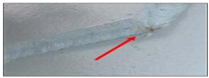
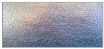
In this work, we analyzed 10 typical types of ship coating defects, including holiday coating, sagging, orange skin, cracking, exudation, wrinkling, bitty appearance, blistering, pinholing and delamination. The number of defect images acquired for each coating defect varies, in which the maximum number of defect images (orange skin) is as high as 759 while the minimum (holiday coating) is as low as 3, as shown in Table 7. The problem of coating defect classification is an unbalanced data classification problem. Before conducting the experiments, we divided the original dataset into a training set, a testing set and a validation set at a ratio of 0.7:0.15:0.15. Subsequently, one-hot coding was performed for 10 defect classes, and due to the different size ratios of the original ship coating defect images collected, the size of each image was adjusted to 128 × 128 × 3. In addition to the above, the data normalization process was used for improving the performance of the neural network.
Table 7.
The unbalanced dataset of the ship coating defects.
3.2. Experimental Environment
The hardware platform used in this experiment is an 11th Gen Intel (R) Core (TM) i5-11400H @ 2.70 GHz with NVIDIA GeForce RTX 3050 Laptop GPU and 16.0 GB RAM. The programming language is Python, version is 3.7.4.
3.3. Evaluation Metrics
In our experiments, we quantitatively analyzed classification results using six common metrics of the confusion matrix, namely accuracy, precision, recall, specificity, F1 Score, G mean, FPR and AUC. The binary classification confusion matrix is shown in Table 8.
Table 8.
The binary classification confusion matrix.
Accuracy and recall are complementary, and the higher these two metrics are, the better. Accuracy is the most intuitive indicator of model performance, and precision is the ratio of positive observations correctly predicted to the total positive observations predicted. F1 score is the harmonic mean of precision and recall rates. It takes both precision and recall into account and is often used as a statistical measure to evaluate the performance of classifiers. G mean is the geometric mean of recall and specificity. For unbalanced datasets, F1 score and G mean can be more effective for evaluating the performance of the model. FPR is the probability that all negative examples are predicted to be positive, and AUC is the area under the ROC curve, which is often used as an important measure of learner performance. These evaluation metrics are defined as follows.
where TP is the true example, TN is the true negative example, FP is the false positive example, and FN is the false negative example.
3.4. Experimental Results and Analysis
3.4.1. Multi-Category Classification Results
In order to vividly demonstrate the effect of DCCVAEACWGAN-GP-generated data and prove the validity of the generated model, we compare the multi-classification results of ship painting defect categories when trained with real datasets, datasets generated by traditional data enhancement methods and datasets generated by the model in this paper. A confusion matrix is usually used to intuitively represent the number of accurate predictions and the number of misclassifications for each category in the test results. The true attributes of the data are represented by the vertical axis, and the predicted state is represented by the horizontal axis. The principal diagonal elements represent the number of samples correctly classified by each defect category, and the remaining elements except for the main diagonal elements represent the number of samples incorrectly classified into other defect categories, as shown in Figure 7. The detection accuracies of each category in Figure 7a are 0.333, 0.733, 0.841, 0.727, 0.69, 0.732, 0.25, 0.657, 0.346 and 0.25, respectively, with an overall accuracy of 0.776. The accuracies of each category in Figure 7b are 0.798, 0.923, 0.845, 0.879, 0.826, 0.858, 0.885, 0.839, 0.882 and 0.891, respectively, with an overall accuracy of 0.866 while the accuracy of each category in Figure 7c is 0.894, 0.973, 0.949, 0.953, 0.928, 0.937, 0.964, 0.946, 0.959 and 0.968, respectively, with an overall accuracy of 0.949. Therefore, the above results indicate that the classification of each category using the data generated by the model in this paper is generally better than that generated using the original actual data and using traditional data augmentation methods, and the overall accuracy of the tested classification is also higher.
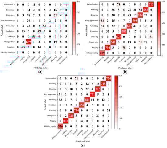
Figure 7.
Overall category-wise confusion matrix comparison between OURS and traditional data augmentation method: (a) Confusion matrix for the original imbalanced dataset. (b) Confusion matrix for balanced datasets augmented by traditional data augmentation methods. (c) The confusion matrix for balanced dataset augmented by our proposed method.
3.4.2. AUC Performance Comparison of Different Data Enhancement Methods
To demonstrate the superiority of the proposed method, we compared the AUC performance of the DCCVAE-ACWGAN-GP with several popularly used data enhancement methods, including SMOTE, Borderline-SMOTE, ADASYN, VAE, CAE, CVAE, GAN, OCGAN and ACGAN. The experimental results are shown in Figure 8.
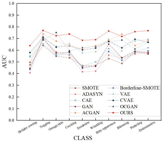
Figure 8.
Comparison of AUC performance on overall categories for OURS and current advanced data enhancement methods.
Although the AUC values of the proposed method in this paper are slightly lower than those of OCGAN and ACGAN in orange skin and blistering, respectively, the AUC values are generally high in other defect classes. The other methods only have high AUC values for one or two defects and significantly low values for other defects (for example, OCGAN is high only for orange skin defects), reflecting the low performance of other data enhancement methods in the face of unbalanced data, as shown in Figure 8. Based on the analysis of the above results, it can be concluded that the performance of the data enhancement algorithm proposed in this paper can better solve the problem of data imbalance and improve the performance of the training model compared with the performance of the current advanced data enhancement methods in sample generation.
3.4.3. The Effect of Removing Class Labels of the Encoder in the DCCVAE
The encoder is able to encode the information contained in the input data while ignoring the changes contained in the class label C. The iterative curve of the DCCVAE versus mean square error with the number of iterations is illustrated in Figure 9. In the first case, we use class labels as input conditions, while in the second, it is the opposite. It can be seen from Figure 9 that the two configured networks reach a fairly stable error value after 37 epochs. Although training the network with class labels can make the learning process more stable, we can employ such unsupervised learning methods to overcome the problems associated with annotations because they allow us to train the model without providing explicit information about the class label C.
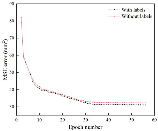
Figure 9.
The iterative curve of DCCVAE means square error with the iteration number.
In this work, we only add information about the class label C in the decoding phase, so that only the conditional probability of the decoder is associated with C while the encoder part remains unchanged, which is more conducive to feature extraction in the encoding phase.
3.4.4. The Curves of Accuracy and Loss Function with Iteration Number
Figure 10 shows the curves of accuracy and loss rate with the number of iterations for the training and test sets. It can be seen from Figure 10 that it is stable in terms of accuracy and loss rate when the number of iterations reaches 998. At this time, the average accuracies of the training set and test set were 94.18% and 92.52%, respectively, and the loss rates were 0.0319 and 0.1120, respectively.
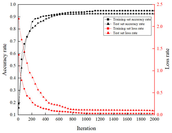
Figure 10.
Iteration curves of accuracy and loss rate of training and test sets with the number of iterations.
3.4.5. The Effect of Hyperparameter Settings on the Model Performance
Because different settings of the weight coefficients of each loss function will have different effects on the performance of the model proposed in this paper, the effects of the weight coefficients of reconstruction loss (β), generative adversarial network loss (ψ), gradient penalty loss (Υ) and classification loss (λ) on the performance of the model are investigated and analyzed in this section. The experimental results are shown in Figure 11. The results show that the performance of DCCVAE-ACWGAN-GP is relatively stable with the variation of ψ and λ, while too large β and too small Υ will degrade the performance seriously.
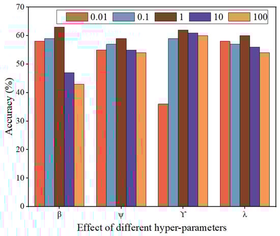
Figure 11.
Effectiveness analysis of the weight coefficients of different loss functions on the performance of the proposed model.
3.4.6. Comparative Analysis of Classification Performance of Different Classifiers
Since the performance of classifier directly affects the classification result, it is crucial to choose a classifier. Therefore, after comparing different data enhancement methods to balance a few classes of ship painting defect images, the scikit learning library was used to import different machine learning classification algorithm modules, such as support vector machine (SVM), random forest (RF), GBDT, decision tree (DT), naive Bayes (NB), k-nearest neighbor (KNN) and artificial neural network (ANN) as classifiers for ship painting defects.
Figure 12 shows radar plots that are used to compare the performance of these classifiers. The large variation in their accuracy, F score and G mean values when using the other classification algorithm modules on both real and artificially generated samples indicates that these classification algorithm modules do not combine well with the generative model proposed in this paper and their performance is not stable. The combination of the classifier proposed in this paper with the DCCVAE-ACWGAN-GP generative model gives the best results both on real samples and on artificially generated samples, with significantly higher accuracy, F score and G mean values. This proves that the proposed method in this paper outperforms other machine learning classifiers for multi-classification in ship painting defect image recognition and improves the overall classification performance of ship painting defect images.
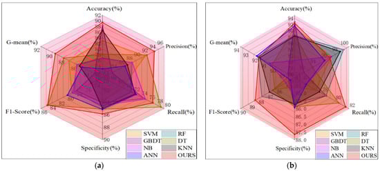
Figure 12.
Comparison of different classification models: (a) real samples, (b) artificially generated samples.
3.4.7. Visual Analysis of Potential Spatial Feature Extraction Capability
In this subsection, in order to perform robustness analysis on the generated painting defect data and visualize the clustering effect of different classes of painting defect data to further illustrate the effectiveness of the generative power of the method, we verify the rationality and effectiveness of our method from an intuitive perspective by reducing the dimensionality of 10 ship painting defect image feature vectors extracted based on encoders and mapping them to a two-dimensional space by a popular high-dimensional visualization data dimensionality reduction algorithm—distributed stochastic neighbor embedding (t-SNE), as shown in Figure 13a–c, respectively. Figure 13a shows the distribution of features extracted from different defect categories obtained from the original imbalance data as the input of the DCCVAE encoder. From Figure 13a, it can be seen that the features extracted from the imbalance data through the DCCVAE encoder are chaotic and overlap with each other, which makes them easy to misclassify as other categories and thus difficult to distinguish. One possible reason is that there are plentiful redundant and invalid features in unbalanced coating defect datasets. Conversely, as shown in Figure 13b, the feature distribution extracted from samples balanced by the DCCVAE is greatly different, and the overlapping parts are less than those in Figure 13a, which means the classification performance is better. Furthermore, the same class samples generated by the DCCVAEACWGAN-GP in Figure 13c have been well combined together, which effectively reduces intra-class changes, and the extracted feature distribution is more compact, while avoiding confusion with inter-class changes, thus improving the accuracy and robustness of detection. Therefore, the experimental results show that the data generated by the model proposed in this paper have more real distribution characteristics. The potential vector z learned by the DCCVAE potential space makes the features extracted by the model more discriminative, which can effectively distinguish different defects and improve the classification performance.
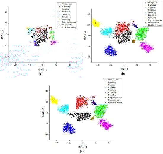
Figure 13.
Visualization of distributions of features comparisons by t-SNE: (a) Original unbalanced data. (b) Data balanced by CVAE. (c) Data balanced by DCCVAE-ACWGAN-GP.
4. Conclusions and Future Work
In this paper, a novel deep learning method for unbalanced ship coating defects classification based on DCCVAEACWGAN-GP is proposed to solve the problems caused by class imbalance and deep generated model for the first time. The experimental results show that the Accuracy, F score and G mean values of the method proposed in this paper are significantly improved. Meanwhile, the performance of the data enhancement algorithm proposed in this paper can better solve the problem of data imbalance and improve the performance of the training model compared with the current advanced data enhancement methods in terms of sample generation. With these results, we can conclude that the unbalanced ship coating defects could be easily classified by using DCCVAE-ACWGAN-GP model for augmenting the classes with fewer samples, even when faced with the class imbalance problem, which can better realize the high precision detection and identification of ship painting defects under small samples conditions. It can provide effective theoretical and technical support for the intelligent detection of ship painting defects and has high engineering research value and application prospects.
Currently, the method’s feasibility has only been verified on the ship defect dataset, and no experiments have been carried out on other datasets to illustrate the general applicability of the method, so in the follow-up work, we will consider verifying the effectiveness and robustness of the proposed method on larger and more diverse datasets.
In addition, since the generative adversarial network proposed in this paper solves the pattern collapse problem to some extent, but only uses a generator and a discriminator, which may lead to the low quality and diversity of the generated samples, the ideas of selective ensemble learning and evolutionary generative adversarial network will be introduced in the future to improve the quality and diversity of the generated samples and improve the overall performance of the model.
Author Contributions
H.B. revised the paper and completed it, T.Y. wrote the first draft of the paper, C.H., X.Z. and Z.G. collected and sorted the data, H.Z. financial support. All authors have read and agreed to the published version of the manuscript.
Funding
The authors gratefully acknowledge the financial support from the Ministry of Industry and Information Technology High-Tech Ship Research Project: Research on the Development and Application of a Digital Process Design System for Ship Coating (No.: MC-202003-Z01-02), the National Defense Basic Scientific Research Project: Research and Development of an Intelligent Methanol-Fueled New Energy Ship (No.: JCKY2021414B011), and the RO-RO Passenger Ship Efficient Construction Process and Key Technology Research (No.: CJ07N20).
Institutional Review Board Statement
Not applicable.
Informed Consent Statement
Not applicable.
Data Availability Statement
The data that support the findings of this study are available from the corresponding author upon reasonable request.
Conflicts of Interest
The authors declare that there are no conflicts of interest regarding the publication of this work.
References
- Bu, H.; Yuan, X.; Niu, J.; Yu, W.; Ji, X.; Lyu, Y.; Zhou, H. Ship Painting Process Design Based on IDBSACN-RF. Coatings 2021, 11, 1458. [Google Scholar] [CrossRef]
- Bu, H.; Ji, X.; Yuan, X.; Han, Z.; Li, L.; Yan, Z. Calculation of coating consumption quota for ship painting: A CS-GBRT approach. J. Coat. Technol. Res. 2020, 376, 1. [Google Scholar] [CrossRef]
- Yuan, X.; Bu, H.; Niu, J.; Yu, W.; Zhou, H. Coating matching recommendation based on improved fuzzy comprehensive evaluation and collaborative filtering algorithm. Sci. Rep. 2021, 11, 14035. [Google Scholar] [CrossRef]
- Ma, H.; Lee, S. Smart System to Detect Painting Defects in Shipyards: Vision AI and a DeepLearning Approach. Appl. Sci. 2022, 12, 2412. [Google Scholar] [CrossRef]
- Bu, H.; Ji, X.; Zhang, J.; Lyu, Y.; Pang, B.; Zhou, H. A Knowledge Acquisition Method of Ship Coating Defects Based on IHQGA-RS. Coatings 2022, 12, 292. [Google Scholar] [CrossRef]
- Chris, A.K.; Fatemeh, A.; Hyeju, S.; Matthew, D.; Hall, P. Data-driven prediction of antiviral peptides based on periodicities of amino acid properties. Comput. Aided Chem. Eng. 2021, 50, 2019–2024. [Google Scholar] [CrossRef]
- Na, D.; Qiang, Y.; Meng, D.; Jian, F.; Xiao, M. A novel feature fusion based deep learning framework for white blood cell classification. J. Ambient. Intell. Humaniz. Comput. 2022, 14, 9839. [Google Scholar] [CrossRef]
- Ryan, M.C.; Mateen, R. Deep learning for image classification. In Proceedings of the 2020 2nd International Conference on Information Technology and Computer Application (ITCA), Guangzhou, China, 18–20 December 2020. [Google Scholar]
- Sadgrove, E.J.; Greg, F.; David, M.; David, W.L. The Segmented Colour Feature Extreme Learning Machine: Applications in Agricultural Robotics. Agronomy 2021, 11, 2290. [Google Scholar] [CrossRef]
- Maiti, A.; Chatterjee, B.; Santosh, C.K. Skin Cancer Classification Through Quantized Color Features and Generative Adversarial Network. Int. J. Ambient. Comput. Intell. 2021, 12, 75–97. [Google Scholar] [CrossRef]
- Yao, W.; Mishal, S. Design of Artistic Creation Style Extraction Model Based on Color Feature Data. Math. Probl. Eng. 2022, 481, 1191. [Google Scholar] [CrossRef]
- Rao, M.A.; Fahad, S.K.; Jorma, L. Compact Deep Color Features for Remote Sensing Scene Classification. Neural Process. Lett. 2021, 53, 1. [Google Scholar] [CrossRef]
- Wang, X.; Zhang, J. An Improved Automatic Shape Feature Extraction Method Based on Template Matching. J. Phys. Conf. Ser. 2021, 2095, 012053. [Google Scholar] [CrossRef]
- Wang, F.; Xu, Z.C.; Shi, Q.S. Integrated Method for Road Extraction: Deep Convolutional Neural Network Based on Shape Features and Images. J. Nanoelectron. 2021, 16, 1011–1019. [Google Scholar] [CrossRef]
- Ravi, D.; Deboleena, S.; Ramakrishnan, S. Rotational moment shape feature extraction and decision tree based discrimination of mild cognitive impairment conditions using mr image processing. Biomed. Sci. Instrum. 2021, 57, 228–233. [Google Scholar] [CrossRef]
- Islam, S.M.; Pinki, F.T. Colour, Texture, and Shape Features based Object Recognition Using Distance Measures. Int. J. Eng. Manuf. 2021, 11, 42–50. [Google Scholar] [CrossRef]
- Wang, Z.; Hu, M.; Zeng, M.; Wang, G. Intelligent Image Diagnosis of Pneumoconiosis Based on Wavelet Transform-Derived Texture Features. Comput. Math. Methods Med. 2022, 2022, 2037019. [Google Scholar] [CrossRef]
- Ong, K.; Young, D.M.; Sulaiman, S.; Shamsuddin, S.M.; Mohd Zain, R.M.; Hashim, H.; Yuen, K.; Sanders, S.J.; Yu, W.; Hang, S. Detection of subtle white matter lesions in MRI through texture feature extraction and boundary delineation using an embedded clustering strategy. Sci. Rep. 2022, 12, 4433. [Google Scholar] [CrossRef]
- Alireza, R.; Yasamin, J.; Ali, K. Explainable Ensemble Machine Learning for Breast Cancer Diagnosis Based on Ultrasound Image Texture Features. Forecasting 2022, 4, 262. [Google Scholar] [CrossRef]
- Jayesh, G.M.; Anto, S.D.; Binil, K.K.; KS, A. Breast cancer detection in mammogram: Combining modified CNN and texture feature based approach. J. Ambient. Intell. Humaniz. Comput. 2022, 14, 11397. [Google Scholar] [CrossRef]
- Kurniastuti, I.; Yuliati, E.N.I.; Yudianto, F.; Wulan, T.D. Determination of Hue Saturation Value (HSV) color feature in kidney histology image. J. Phys. Conf. Ser. 2022, 2157, 012020. [Google Scholar] [CrossRef]
- Panagiotis, K.; Gerasimos, T.; Boulougouris, E. Environmental-economic sustainability of hydrogen and ammonia fuels for short sea shipping operations. Int. J. Hydrogen Energy 2024, 57, 1070–1080. [Google Scholar] [CrossRef]
- Na, H.J.; Park, J.S. Accented Speech Recognition Based on End-to-End Domain Adversarial Training of Neural Networks. Appl. Sci. 2021, 11, 8412. [Google Scholar] [CrossRef]
- Siraj, K.; Muhammad, S.; Tanveer, H.; Amin, U.; Ali, S.I. A Review on Traditional Machine Learning and Deep Learning Models for WBCs Classification in Blood Smear Images. IEEE Access 2021, 9, 1065. [Google Scholar] [CrossRef]
- Ding, H.; Chen, H.; Dong, L.; Fu, Z.; Cui, X. Imbalanced data classification: A KNN and generative adversarial networks-based hybrid approach for intrusion detection. Future Gener. Comput. Syst. 2022, 131, 240–254. [Google Scholar] [CrossRef]
- Du, C.; Liu, P.; Zheng, M. Classification of Imbalanced Electrocardiosignal Data using Convolutional Neural Network. Comput. Methods Programs Biomed. 2022, 214, 106483. [Google Scholar] [CrossRef] [PubMed]
- Athanasios, A.; Nikolaos, D.; Anastasios, D.; Eftychios, P. Deep Learning for Computer Vision: A Brief Review. Comput. Intell. Neurosci. 2018, 2018, 7068349. [Google Scholar] [CrossRef]
- Young, T.; Hazarika, D.; Poria, S.; Cambria, E. Recent Trends in Deep Learning Based Natural Language Processing [Review Article]. IEEE. Comput. Intell. Mag. 2018, 13, 55. [Google Scholar] [CrossRef]
- Estiri, S.N.; Jalilvand, A.H.; Naderi, S.; Najafi, M.H.; Fazeli, M. A Low-Cost Stochastic Computing-based Fuzzy Filtering for Image Noise Reduction. In Proceedings of the IEEE 13th International Green and Sustainable Computing Conference (IGSC), Pittsburgh, PA, USA, 24–25 October 2022; pp. 1–6. [Google Scholar]
- Zhao, W.; Qin, W.; Li, M. An Optimized Model based on Metric-Learning for Few-Shot Classification. In Proceedings of the 33rd Chinese Control and Decision Conference (CCDC), Kunming, China, 22–24 May 2021; pp. 336–341. [Google Scholar]
- Park, S.; Zhong, R.R. Pattern Recognition of Travel Mobility in a City Destination: Application of Network Motif Analytics. J. Travel Res. 2022, 61, 1201. [Google Scholar] [CrossRef]
- Liu, J.; Zhang, K.; Wu, S.; Shi, H.; Zhao, J.; Yao, D. An Investigation of a Multidimensional CNN Combined with an Attention Mechanism Model to Resolve Small-Sample Problems in Hyperspectral Image Classification. Remote Sens. 2022, 14, 785. [Google Scholar] [CrossRef]
- Dong, Y.; Li, Y.; Zheng, H.; Wang, R.; Xu, M. A new dynamic model and transfer learning based intelligent fault diagnosis framework for rolling element bearings race faults: Solving the small sample problem. ISA Trans. 2021, 121, 327. [Google Scholar] [CrossRef]
- Gao, H.; Yao, Y.; Li, C.; Zhang, X.; Zhao, J.; Yao, D. Convolutional neural network for spectral–spatial classification of hyperspectral images. Neural Comput. Appl. 2019, 31, 8997. [Google Scholar] [CrossRef]
- Sukarna, B.; Monirul, I.; Yao, X.; Kazuyuki, M. MWMOTE-Majority Weighted Minority Oversampling Technique for Imbalanced Data Set Learning. IEEE Trans. Knowl. Data Eng. 2014, 26, 405. [Google Scholar] [CrossRef]
- Ji, X.; Wang, J.; LI, Y.; Sun, Q.; Jin, S.; Tony, Q.S. Quek. Data-Limited Modulation Classification with a CVAE-Enhanced Learning Model. IEEE Commun. 2020, 24, 1. [Google Scholar] [CrossRef]
- Feng, X.; Shen, Y.; Wang, D. A Survey on the Development of Image Data Augmentation. Comput. Sci. Appl. 2021, 11, 370. [Google Scholar] [CrossRef]
- Waheed, A.; Goyal, M.; Gupta, D.; Khanna, A.; Turjman, F.A.; Pinheiro, P.R. CovidGAN: Data Augmentation Using Auxiliary Classifier GAN for Improved Covid-19 Detection. IEEE Access 2020, 8, 91916. [Google Scholar] [CrossRef]
- Jong, P.Y.; Woosang, C.S.; Gyogwon, K.; Kim, M.S.; Lee, C.; Lee, S.J. Automated defect inspection system for metal surfaces based on deep learning and data augmentation. J. Manuf Syst. 2020, 55, 324. [Google Scholar] [CrossRef]
- Aqib, H.A.M.; Nurlaila, I.; Ihsan, Y.; Mohd, N.T. VGG16 for Plant Image Classification with Transfer Learning and Data Augmentation. Int. J. Eng. Technol. 2018, 7, 4. [Google Scholar] [CrossRef]
- Sohn, Y.K.; Yan, X.; Lee, H. Learning structured output representation using deep conditional generative models. In Proceedings of the 28th International Conference on Neural Information Processing Systems, Bali, Indonesia, 8–12 December 2021; pp. 3483–3491. [Google Scholar]
- Wu, X.; Feng, W.; Guo, Y.; Wang, Q. Feature Learning for SAR Target Recognition with Unknown Classes by Using CVAE-GAN. Remote Sens. 2021, 13, 3554. [Google Scholar] [CrossRef]
- Yang, H.; Lu, X.; Wang, S.; LU, Z.; Yao, J.; Jiang, Y.; Qian, J. Synthesizing Multi-Contrast MR Images Via Novel 3D Conditional Variational Auto-Encoding GAN. Mob. Netw. Appl. 2021, 26, 415–424. [Google Scholar] [CrossRef]
- Divya, S.; Tarun, T.; Cao, J.; Zhang, C. Multi-Constraint Adversarial Networks for Unsupervised Image-to-Image Translation. Conf. Inf. Process. 2022, 31, 1601. [Google Scholar] [CrossRef]
- Christian, L.; Lucas, T.; Ferencr, H.; Jose, C.; Andrew, P.; Alykhan, T.; Johannes, T.; Wang, Z.; Shi, W. Photo-Realistic Single Image Super-Resolution Using a Generative Adversarial Network. In Proceedings of the Conference on Computer Vision and Pattern Recognition (CVPR), Honolulu, HI, USA, 21–26 July 2017; pp. 1063–6919. [Google Scholar]
- Zhou, Q.; Zhou, W.; Yang, B.; Jun, H. Deep cycle autoencoder for unsupervised domain adaptation with generative adversarial networks. IET Comput. Vis. 2019, 13, 659. [Google Scholar] [CrossRef]
- Khalil, M.A.; Sadeghiamirshahidi, M.; Joeckel, R.; Santos, F.M.; Riahi, A. Mapping a hazardous abandoned gypsum mine using self-potential, electrical resistivity tomography, and Frequency Domain Electromagnetic methods. J. Appl. Geophys. 2022, 205, 104771. [Google Scholar] [CrossRef]
- Ngoc, T.T.; Viet, H.T.; Ngoc, B.N.; Ngai, M.C. An Improved Selfsupervised GAN via Adversarial Training. In Proceedings of the Computer Vision and Pattern Recognition, Long Beach, CA, USA, 14 May 2019. [Google Scholar]
- Santiago, L.T.; Alice, C.; Rafael, M.; Aggelos, K.K. A single video superresolution GAN for multiple downsampling operators based on pseudo-inverse image formation models. Digit Signal Process. 2020, 104, 102801. [Google Scholar] [CrossRef]
- Jang, Y.; Sim, J.; Yang, J.; Kwon, N.K. Improving heart rate variability information consistency in Doppler cardiogram using signal reconstruction system with deep learning for Contact-free heartbeat monitoring. Biomed. Signal Process Control. 2022, 76, 103697. [Google Scholar] [CrossRef]
- Zou, L.; Zhang, H.; Wang, C.; Wu, F.; Gu, F. MW-ACGAN: Generating Multiscale High-Resolution SAR Images for Ship Detection. Sensors 2020, 20, 6673. [Google Scholar] [CrossRef]
- Ugo, F.; Alfredo, D.S.; Francesca, P.; Paolo, Z.; Francesco, P. Using generative adversarial networks for improving classification effectiveness in credit card fraud detection. Inf. Sci. 2017, 479, 448. [Google Scholar] [CrossRef]
- Augustus, O.; Christopher, O.; Jonathon, S. Conditional Image Synthesis With Auxiliary Classifier GANs. In Proceedings of the Computer Vision and Pattern Recognition, Honolulu, HI, USA, 20 July 2017. [Google Scholar]
- Pan, Z.; Yu, W.; Wang, B.; Xie, H.; Sheng, V.; Lei, J.; Kwong, S. Loss Functions of Generative Adversarial Networks (GANs): Opportunities and Challenges. IEEE Trans. Emerg. Topics Comput. 2020, 4, 500. [Google Scholar] [CrossRef]
- Demir, S.; Krystof, M.; Koen, K.; Nikolaos, G.P. Data augmentation for time series regression: Applying transformations, autoencoders and adversarial networks to electricity price forecasting. Appl. Energy 2021, 304, 117695. [Google Scholar] [CrossRef]
Disclaimer/Publisher’s Note: The statements, opinions and data contained in all publications are solely those of the individual author(s) and contributor(s) and not of MDPI and/or the editor(s). MDPI and/or the editor(s) disclaim responsibility for any injury to people or property resulting from any ideas, methods, instructions or products referred to in the content. |
© 2024 by the authors. Licensee MDPI, Basel, Switzerland. This article is an open access article distributed under the terms and conditions of the Creative Commons Attribution (CC BY) license (https://creativecommons.org/licenses/by/4.0/).