Abstract
An accurate and stable prediction of the corrosion rate of natural gas pipelines has a major impact on pipeline material selection, inhibitor filling process, and maintenance schedules. At present, corrosion data are impacted by non-linearity and noise interference. The traditional corrosion rate prediction methods often ignore noise data, and only a small number of researchers have carried out in-depth research on non-linear data processing. Therefore, an innovative hybrid prediction model has been proposed with four processes: data preprocessing, optimization, prediction, and evaluation. In the proposed model, a decomposing algorithm is applied to eliminate redundant noise and to extract the primary characteristics of the corrosion data. Stratified sampling is applied to separate the training set and the test set to avoid deviation due to the sampling randomness of small samples. An improved particle swarm optimization algorithm is applied to optimize the parameters of support vector regression. A comprehensive evaluation of this framework is also conducted. For natural gas pipelines in southwest China, the coefficient of determination and mean absolute percentage error of the proposed hybrid model are 0.925 and 5.73%, respectively, with better prediction performance compared to state-of-the-art models. The results demonstrate the best approach for improving the prediction accuracy of the proposed hybrid model. This can be applied to improve the corrosion control effect and to support the digital transformation of the corrosion industry.
1. Introduction
Widely considered an essential strategic reserve material, natural gas is mainly transported through pipelines. Due to the features of the transportation medium, operating environment, service life, etc., the pipelines for natural gas are subject to deterioration and degradation as a result of a series of corrosion mechanisms [1]. According to statistics compiled by the European Gas Pipeline Incident Data Group (EGIG), 25% of natural gas pipeline failures are caused by corrosion, as shown in Figure 1. Corrosion is one of the main causes of natural gas pipeline failure. It can damage the normal operation of the pipeline and even lead to major safety accidents [2,3]. Determining accurate corrosion rates can aid in accurately predicting the failure of natural gas pipelines. Moreover, it can provide scientific guidance for both decision making and corrosion risk management regarding natural gas pipelines [4]. Many gas fields in China and around the world are implementing a gradual digital transformation. Predicting an accurate corrosion rate is a core aspect of this digital transformation.
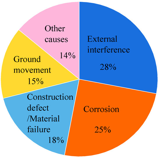
Figure 1.
Causes of natural gas pipeline failures.
Pipeline operations are characterized by non-stationarity, non-linear fluctuation, and complexity, which cause information redundancy, noisy data, and non-linearity in the data [5]. Traditional prediction methods ignore information redundancy and noisy data, with the non-linear data processing of these methods being simplistic. Due to these shortcomings, corrosion rate prediction has become complicated and challenging. To address these issues, some researchers have focused on corrosion rate analysis and prediction in recent years and have proposed various methods. These methods consist of four types: physical, statistical, artificial intelligence (AI), and hybrid [2,6,7].
In 1947, Schneider applied the physical method to studies on corrosion to estimate the lifespan of pipelines [8]. The three conservation formulas used for examining corrosion and the law of thermodynamics were the basic foundations for this approach. This method has been employed frequently to assess natural gas pipeline corrosion. The results are often applicable and precise when using this method to forecast corrosion based on extensive parameter information. However, as it depends on a large number of physical parameters, modeling expenses are considerable, and calculation efficiency is low. In addition, it is often difficult for this method to converge rapidly.
The results of typical corrosion prediction cases based upon physical and statistical methods are shown in Table 1. Statistical methods are applied to build prediction models that are based on actual corrosion rate data, such as linear regression (LR) [9], autoregressive moving average (ARMA) [10], autoregressive integrated moving average (ARIMA) [11], and grey model (GM) [12]. In actual production conditions, statistical methods are mostly used for corrosion rate prediction. However, these methods have drawbacks including poor extrapolation capabilities, a limited prediction range, and a dependency on robust data. Due to the aforementioned drawbacks, statistical methods are better suited to linear data, and prediction outcomes frequently fall short of the requisite precision.

Table 1.
Summary of typical corrosion prediction cases using statistical and physical methods.
Soft-computing approaches have developed quickly in recent years [13,14,15], with AI methods such as neural networks (NNs) [16,17] and support vector machines (SVMs) [18,19,20] being routinely utilized for corrosion prediction. As AI methods include solid fault tolerance, they have outstanding prediction performance. The results of corrosion prediction examples based on the above two methods are shown in Table 2. The results demonstrate that SVMs have an excellent generalization ability, and their prediction performance is better than that of NNs, even with small samples [1,21,22].
Table 2.
The results of corrosion prediction examples using AI methods.
In addition, applied research has shown that the reasonable combination of hyper-parameters will make SVM training faster and the prediction results more accurate [23]. The results of corrosion prediction cases based upon hybrid methods are shown in Table 3. Many intelligent optimization algorithms are utilized in prediction and classification to optimize the hyper-parameters of SVMs. These algorithms include the firefly algorithm [24], particle swarm optimization (PSO) [21,25], genetic algorithm (GA) [26], coupled simulated annealing algorithm (CSA) [27], artificial bee colony algorithm [1], multi-objective salp swarm algorithm (MOSSA) [28], and artificial fish-swarm algorithm (AFSA) [29]. Of the various optimization algorithms, PSO can perform demanding optimization tasks. This ability is conducive to identifying a reasonable solution. However, PSO is prone to phenomena such as local optimal solutions and premature convergence. The improved PSO algorithm is therefore applied to address these shortcomings. Unfortunately, the above hybrid prediction methods ignore noisy data, which cause the complex relationships between non-stationary and non-linear data series to be captured inaccurately, making the final prediction effect unsatisfactory.
Table 3.
The results of corrosion prediction cases using hybrid methods.
In recent years, applied research has proven that the decomposition algorithm can enhance the prediction accuracy of models by decomposing the original data series into several sub-layers. Therefore, to handle the non-stationarity and non-linearity of data series, many researchers have introduced different data decomposition techniques. Some data decomposition techniques have been incorporated into hybrid models to identify and extract the main features of data series. These include the wavelet transform (WT) [30], wavelet packet transform (WPT) [31], empirical mode decomposition (EMD) [32], and ensemble empirical mode decomposition (EEMD) [33]. Through the data decomposition techniques, significant characteristics of the original data series are captured, and the model’s prediction accuracy is improved.
To solve the previously mentioned problems, a novel hybrid model is proposed for the corrosion rate prediction of natural gas pipelines. The model is proposed on the basis of the complete ensemble empirical mode decomposition with adaptive noise (CEEMDAN) and the support vector machine (SVM) optimized by the improved PSO. Overall, the proposed method combines advanced prediction model functions, optimization algorithms, decomposition technologies, and evaluation modules. Through the proposed model, the negative impact of noise can be eliminated, inherent characteristics of the original data can be captured, and ideal prediction results can be obtained.
The system includes data preprocessing, optimization, prediction, and evaluation. Specifically, CEEMDAN is employed to decompose the original data series into multiple intrinsic mode functions (IMFs) with different frequencies and residuals. This allows the major feature of the original data series to be identified and extracted successfully. Next, the patterns obtained by CEEMDAN are used as input features. Then, SVM optimized by IPSO is used to predict the patterns. Finally, the evaluation module is applied to comprehensively evaluate the proposed hybrid system. The evaluation module comprises seven typical measurement rules, prediction effectiveness, Grey relational analysis, and the Taylor diagram.
Compared with previous methods, the novelty and contribution of the proposed model are (1) CEEMDAN are adopted to solve the forecasting difficulties of the high-frequency signal, so that the main features of the original data series can be successfully identified and extracted. (2) The IPSO is used to solve the shortcomings of local optimal solutions and premature convergence in the traditional PSO, and then used to optimize the hyper-parameters of SVM. (3) The stratified sampling method is adopted to divide the training set and the test set, thus avoiding the sampling stochasticity of small samples. (4) Seven typical measurement rules, prediction effectiveness, Grey relational analysis, and the Taylor diagram are adopted to conduct a persuasive evaluation for the proposed hybrid system.
The remainder of this paper is arranged as follows: Section 2 describes the individual methods applied in the paper. Section 3 introduces the established hybrid prediction strategy for corrosion rate prediction. In Section 4, data acquisition and processing are conducted, and the prediction performance of the established hybrid model is compared with that of other benchmark models. A deeper evaluation of the model’s prediction performance is discussed in Section 5. Finally, the conclusions of the study are presented in Section 6.
2. Methods
In this section, the relevant methods applied in the developed prediction framework, such as CEEMDAN, SVM, and IPSO, are introduced.
2.1. Decomposition Technique
The EMD method developed by Huang [34] decomposes the original signals into several IMFs. Due to the incompatibility of the mode and EMD, Wu and Huang [35] established the EEMD method. EEMD demonstrates an obvious improvement in stability, but it fails to offset the added noise completely. Therefore, a more advanced data decomposition algorithm called CEEMDAN has been proposed by Torres [36]. The CEEMDAN algorithm not only allows for mode mixing in EMD but also sufficiently eliminates the noise by adding paired white noise. Ultimately, the components achieve lower noise and better prediction results. Therefore, the CEEMDAN algorithm can be used as a practical data preprocessing tool to indirectly improve prediction performance.
2.2. Improved Particle Swarm Optimization–Support Vector Machine (IPSO–SVM)
A five-fold cross-validation error is applied to perform an unbiased estimate of the generalization error, and the IPSO method is applied to optimize the SVM hyper-parameters.
2.2.1. IPSO
In 1995, Kennedy and Eberhart proposed the PSO algorithm [37], which is a global optimization algorithm based on swarm behaviors seen in nature. The PSO algorithm can perform complex optimization tasks and is conducive to the rapid convergence of the model to a reasonable solution. Therefore, the basic PSO and related improvement methods have seen all manner of real-world applications. However, the PSO algorithm is prone to issues such as local optimal solutions and premature convergence. To address this deficiency, an inertial weight ω was introduced to form a new algorithm, i.e., the improved particle swarm algorithm. The larger ω helps particles jump out of the extremum point and perform a global search, while the smaller ω helps the particles conduct a refined search in the current search area to facilitate convergence. Thus, certain methods need to be applied to adjust the inertial weight to achieve a balance between a global search and a refined search.
Based on the influence of inertial weight on the search ability of the PSO algorithm, the following improvements are proposed:
where ωmin is the minimum inertia weight, and kmax is the maximum number of iterations.
According to the sinusoidal variation of ω, the solution process goes through three stages: local optimization around the particle itself, global optimization, and local search of the optimal particles. The specific process is as follows:
Step 1 (population initialization): Initialize the particle swarm and set parameters, such as particle number m, particle dimension n, fitness function, learning factor, and iteration time. Initialize the velocity and position of particles randomly and calculate the local optimal position and the global optimal position of the current particle swarm.
Step 2 (fitness calculation): Determine each particle’s fitness value in accordance with the fitness function.
Step 3 (iterative update of the position and velocity of the particle): Each particle’s current fitness value is compared to its prior best position, and if a better value is found, that location is applied as the particle’s current best position. Compare each particle’s fitness value to the entire particle swarm’s current best position. If a better value is found, it shall be used as the particle’s current best position.
Step 4 (iteration termination): Select the maximum number of iterations or preset accuracy as the iteration termination condition according to the specific condition. If the termination condition is not met, return to step (1) and continue to update the particle’s position and velocity iteratively. Otherwise, end the program to obtain the optimal solution.
2.2.2. SVM
In 1995, SVM was established by Vapnik [38]. The fundamental difference between SVM and ANN is that the former mainly relies on the structural risk minimization principle, whereas the latter operates based on the principle of empirical risk minimization. Even with insufficient data, SVM can avoid issues with over-fitting and maintain outstanding prediction performance. The prediction effect of SVM largely results from the kernel function. Three classic kernel functions exist, namely, polynomial, linear, and Gaussian (RBF). Related research indicates that the RBF kernel function performs better in most cases and has fewer parameters to be considered than other kernel functions. Hence, the RBF kernel function is considered [39,40,41].
3. The Hybrid CEEMDAN–IPSO–SVM Model
Traditional corrosion rate prediction methods ignore information redundancy and noisy data and lack an in-depth consideration of non-linear processes. Therefore, a hybrid prediction model is established based on the decomposition technique and SVM optimized by IPSO. The main parameters of the prediction system are presented in Table 4 according to the functions of each component in the developed prediction system. Using the decomposition technique, the redundant noise in the prediction process can be eliminated, and significant features of the original datasets can be captured effectively. Additionally, this section establishes the improved PSO method based on SVM, which can improve exploration and exploitation capacities, eliminate local optimal solutions, and avoid premature convergence. The flowchart seen in Figure 2 demonstrates the hybrid prediction framework that was developed for the corrosion rate prediction of natural gas pipelines. The reasonable combination of different methods can take advantage of each method’s merits and obtain practical and effective prediction results.
Table 4.
Experimental parameters.
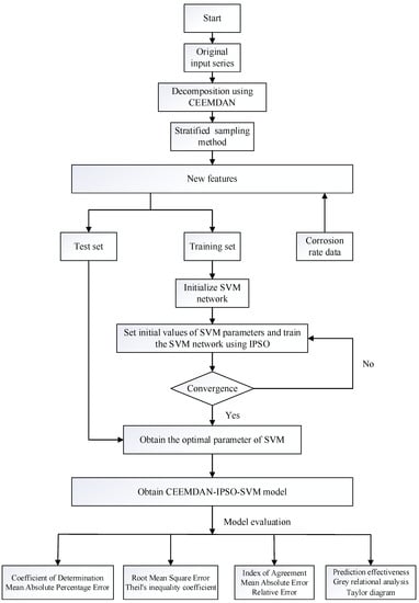
Figure 2.
The flowchart of the hybrid prediction system.
4. Empirical Study
This section provides details regarding data acquisition, the stratified sampling method, performance metrics, and other related research. The performance of the developed hybrid prediction framework has been verified according to the experimental results.
4.1. Data Acquisition
In this paper, natural gas pipelines in southwestern China are used to elaborate the proposed methodology. Sixty sets of corrosion data for natural gas pipelines were acquired from historical reports. There are 10 corrosion-affecting factors in each set of data, and these factors include partial pressure of H2S, kPa, (X1); partial pressure of CO2, kPa, (X2); temperature, °C, (X3); pH value (X4); Cl ion content, mg/L, (X5); wall shear stress (gas phase), Pa, (X6); wall shear stress (liquid phase), Pa, (X7); gas flow rate, m/s, (X8); liquid flow rate, m/s, (X9); and liquid holdup, HOL, (X10).
For the above influencing factors, those influencing the internal corrosion of natural gas pipelines are analyzed as follows:
- Partial pressure (X1 and X2): When the partial pressure of H2S is low, the corrosion rate of steel is also low. With the increase in the partial pressure of H2S, the steel exhibits corrosion characteristics that increase and then decrease. When the CO2 partial pressure increases, the corrosion rate of steel tends to increase monotonically, and the corrosion form is dominated by uniform corrosion.
- Temperature (X3): Temperature is an essential factor affecting corrosion. Other studies have shown that the corrosion rate of metals in acidic solutions usually tends to increase first and then decrease as the temperature rises.
- PH value (X4): As the pH value increases, the corrosion rate shows a significant downward trend. Iron sulfide (Fe8S9) is generated in a solution with a low pH value, which has no protective effect and cannot inhibit the corrosion of steel. As the pH value increases, the FeS content increases, and the FeS film has a certain protective effect that promotes a decrease in the corrosion rate.
- Cl ion content (X5): Cl ions have a strong penetration ability, and they will preferentially adsorb on the surface of the pipeline and interact with it to form soluble compounds, thereby aggravating the corrosion of the pipeline. When the Cl ion concentration is 0% to 3%, the corrosion rate rises faster with the increase in the Cl ion concentration in the water; when the Cl ion concentration is 3% to 6%, the corrosion rate rises more slowly with the addition of the Cl ion concentration in the water.
- Wall shear stress (X6 and X7): Although the flow rate is intuitive and easy to measure, it does not reflect the physical properties of the fluid. The surface shear stress can comprehensively reflect the influence of the fluid’s physical properties, geometric features, and velocity on its motion features. The fluid’s motion described by these parameters can reflect the flow corrosion’s essence better than the flow rate. The surface shear stress is most important since it is directly related to the state of the metal/fluid interface. Surface shear stress is caused by the velocity gradient of the metal surface when the fluid medium is moving. Its size directly measures the degree of interaction between the material surface and the fluid medium.
- Flow rate (X8 and X9): An increase in the flow rate will accelerate the transfer of corrosive substances, reduce the accumulation of corrosive product film on the surface of the sample, and increase the shear stress on the surface of the sample, which will raise the corrosion rate. Such an increase will also cause changes in the morphology and structure of the corrosive product film, resulting in a decrease in the corrosion rate. By combining the two effects, the flow rate increases, and the corrosion rate tends to decrease first and then increase.
- Liquid holdup (X10): In a multiphase flow system, the metal surface can easily form a water film when the liquid phase is relatively large. Acid gas can dissolve quickly in the liquid phase, providing an acid medium that should be conducive to the occurrence of corrosion; however, there is an obvious reduction in the corrosion rate.
Considering that the acquired data parameters include just 10 dimensions, it has been found, through theoretical analysis, that the above parameters significantly impact the corrosion rate. Therefore, the acquired 10-dimensional parameters have been selected as the input values.
Table 5 displays the data on natural gas pipeline corrosion that have been collected in descriptive statistics, including the minimum, maximum, mean, kurtosis, standard deviation, and skewness. To simplify the prediction process, the original data series was first pre-processed by a linear transformation and then normalized to the range of (0,1).
Table 5.
Descriptive corrosion data statistics.
4.2. Stratified Sampling (SS)
In this study, the training set and the test set are split into a 7:3 ratio. Due to the small quantity of initial samples, the distribution rules of the training set and the test set will be substantially different from the distribution rules of the original dataset if the traditional random sampling method is used to separate the overall dataset. Therefore, the SS method is applied to guarantee the objectivity of the prediction outcomes [42,43].
Based on the distribution rule for corrosion rates, the deviations of the training set/test set obtained through random sampling and the training set/test set obtained through SS from the initial samples are shown in Table 6. The mean absolute percentage errors (MAPE) for random sampling and SS are calculated based on the corrosion data of natural gas pipelines. According to the analysis, in terms of the MAPE obtained through random sampling, the MAPE of the training set and the test set is 21.36% and 32.47%, respectively. In terms of the MAPE obtained through the SS method, the MAPE of the training set and the test set is 3.16% and 5.21%, respectively. Thus, it can be concluded that the training set and the test set separated by SS are more consistent with the initial sample in comparison to simple random sampling. It can also be understood that the SS method can prevent obvious sample bias and guarantee the accuracy of the prediction outcomes. Therefore, the SS method is used to separate the training set and the test set.
Table 6.
Comparison of the MAPE obtained through random sampling and SS.
4.3. Performance Metrics
Prediction accuracy is a key index for judging prediction performance. Many indicators of prediction accuracy have been recorded in the literature. To verify the accuracy of the established model, seven typical metric indexes are applied, including RE, MAE, MAPE, RMSE, R2, IA, and TIC [44,45,46]. For a variety of indicators, the closer the values of the evaluation indicators (e.g., RE, MAE, MAPE, RMSE, and TIC) are to 0, the better performance the model has. Furthermore, the closer the values of the indicators, such as R2 and IA, are to 1, the better the model’s performance. The calculation formulas of these performance measures are shown in Table 7.
Table 7.
Performance measures.
4.4. Experimental Results and Analysis
The developed hybrid prediction framework is expressed as CEEMDAN–IPSO–SVM. Different single models, optimization algorithms, and decomposition approaches are considered to validate the generated prediction framework’s advantages, and four experiments are carried out. In experiment I, the predictive performance of SVM and BPNN, two mainstream machine-learning algorithms, are compared to verify the rationality of SVM as the basic model of the hybrid model. In experiment II, two sets of comparative analyses are conducted, including comparing the prediction performance of CEEMDAN–IPSO–SVM and IPSO–SVM and comparing the prediction performance of CEEMDAN–SVM and SVM. This was performed to verify the rationality of selecting CEEMDAN as the decomposition algorithm of the hybrid model. In experiment III, two sets of comparative analyses are conducted, including comparing the prediction performance of IPSO–SVM, PSO–SVM, GA–SVM, and SVM and comparing the prediction performance of CEEMDAN–IPSO–SVM and CEEMDAN–SVM to verify the rationality of selecting IPSO as the optimization algorithm of the hybrid model. Experiment IV assesses the proposed hybrid model in greater depth by comparing CEEMDAN–IPSO–SVM with six models. The best predicted effect is displayed in bold in each row for the minimum values of MAE, RMSE, MAPE, and TIC; the maximum values of R2 and IA; and the closest to the 0 values of RE.
4.4.1. Experiment 1: Select the Appropriate Benchmark Model
Soft-computing approaches have developed quickly in recent years, and AI methods such as ANN and SVM are frequently used to assess corrosion in oil and gas pipelines. Figure 3 displays the benchmark model statistics proportions regarding the above methodologies for the prediction of corrosion in gas and oil pipelines, with the ANN and SVM methods comprising a significant proportion. BPNN is a typical ANN model. Therefore, BPNNs and SVMs are selected as alternative models for the basic model of the hybrid model. A comparative study of BPNN and SVM prediction performance is conducted, and the rationality of SVM as the basic model for the hybrid model is verified. The MAPE and R2 diagrams for the two benchmark models are shown in Figure 4.
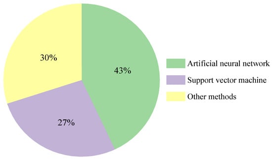
Figure 3.
Statistics proportions of benchmark models for predicting oil and gas pipeline corrosion.
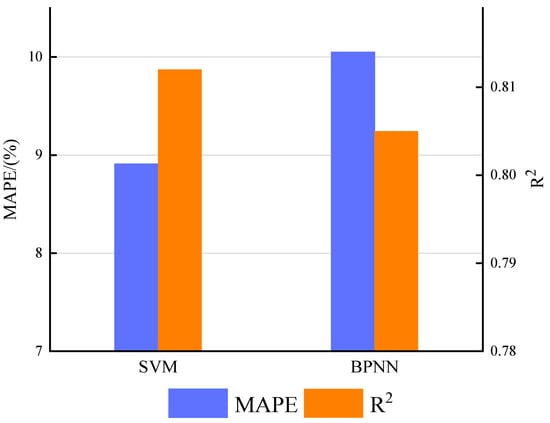
Figure 4.
The MAPE and R2 for the two benchmark models.
By looking at the two indexes in Figure 4, it can be seen that the SVM model is able to achieve the minimum values for MAPE and the maximum values for R2. This demonstrates that the SVM model is an appropriate basic model. Therefore, the SVM model is used as the basic prediction model in the hybrid prediction framework.
4.4.2. Experiment 2: Select the Appropriate Data Decomposition Algorithm
To verify the rationality of selecting CEEMDAN as the decomposition algorithm for the hybrid model, two sets of comparative analysis are conducted. These include comparing the predictive ability between SVM and CEEMDAN–SVM, and comparing the predictive ability between IPSO–SVM and CEEMDAN–IPSO–SVM. The IA and MAE of the compared models are shown in Figure 5.
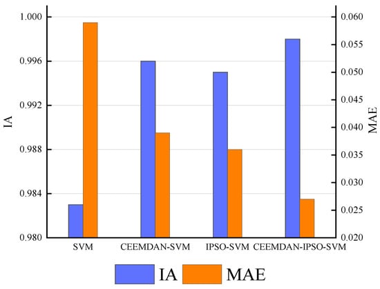
Figure 5.
The IA and MAE for the comparative models.
Figure 5 demonstrates the comparison of predictive ability between SVM and CEEMDAN–SVM. It is found that the CEEMDAN–SVM model can obtain the minimum values of MAE and the maximum values of IA. Moreover, through the comparison of predictive ability between IPSO–SVM and CEEMDAN–IPSO–SVM, it is found that the CEEMDAN–IPSO–SVM can acquire the minimum values of MAE and the maximum values of IA. It is shown that the addition of the CEEMDAN data decomposition algorithm contributes to eliminating redundant noise, capturing the main data features, and improving the model’s prediction accuracy. Therefore, CEEMDAN is used as the data decomposition algorithm in the hybrid prediction framework.
4.4.3. Experiment 3: Select the Appropriate Optimization Algorithm
To verify the rationality of selecting IPSO as the optimization algorithm for the hybrid model, two sets of comparative analysis are conducted. These include comparing the predictive ability between SVM, GA–SVM, PSO–SVM, and IPSO–SVM, and comparing the predictive ability between CEEMDAN–SVM and CEEMDAN–IPSO–SVM. The RMSE and TIC of the compared models are shown in Figure 6.
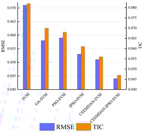
Figure 6.
The RMSE and TIC for the comparative models.
Figure 6 demonstrates the comparison of predictive ability between SVM, GA–SVM, PSO–SVM, and IPSO–SVM. It is found that SVM has the worst prediction effect. IPSO–SVM can obtain the minimum values of RMSE and TIC. It can be concluded that the optimization algorithm can improve prediction accuracy and is essential in corrosion rate prediction. Moreover, through the comparison of predictive ability between CEEMDAN–SVM and CEEMDAN–IPSO–SVM, it is found that CEEMDAN–IPSO–SVM can obtain the minimum values of RMSE and TIC. This proves that the addition of the IPSO algorithm can improve the performance of PSO to a certain degree and effectively solve the issue of the optimization algorithm being prone to an optimal local solution. Therefore, IPSO is used as the data decomposition algorithm in the hybrid prediction framework.
4.4.4. Experiment 4: Compare Different Prediction Models
Based on the three experiments detailed above, a hybrid prediction model called CEEMDAN–VMD–IPSO–SVM is established. A final model comparison is conducted to comprehensively verify the proposed hybrid prediction model’s performance. The detailed prediction errors of the compared models and the proposed hybrid model are listed in Table 8.
Table 8.
Performance measures.
The curves of the actual values, predicted values, and prediction errors for the proposed model are shown in Figure 7. According to the analysis, the hybrid model fits the historical data well, and the relative error (RE) is mostly in the range of [−5%, 5%], which ensures a high degree of suitability.
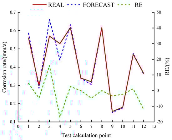
Figure 7.
The curves of the actual values, predicted values, and prediction errors for the proposed model.
To further evaluate the prediction outcome of the hybrid model, the proposed hybrid model is compared with BPNN, SVM, GA–SVM, PSO–SVM, IPSO–SVM, and CEEMDAN–SVM. There are 12 test set groups in the corresponding datasets in the study, and the scatter distribution of relative errors predicted by different models in the range of [−5%, 5%] is shown in Figure 8 and Figure 9. According to seven models, namely BPNN, SVM, GA–SVM, PSO–SVM, IPSO–SVM, CEEMDAN–SVM, and CEEMDAN–IPSO–SVM, the quantity of scatter points in the test set with the relative error of different models falling within the range of [−5%, 5%] is 3, 4, 5, 5, 7, 6, and 9, respectively.
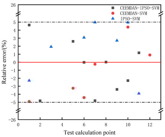
Figure 8.
Scatter distribution results for relative errors predicted by different models.
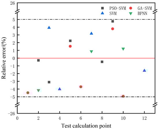
Figure 9.
Scatter distribution results for relative errors predicted by different models.
It can be seen that the relative error predicted by the CEEMDAN–VMD–IPSO–SVM model falls within the range of [−5%, 5%] and has the largest number of scatter points. This proves that the hybrid model has the lowest prediction error and the best prediction accuracy for the small sample corrosion rate.
5. Discussion
In this section, prediction effectiveness (PE), Grey relational analysis (GRA), and the Taylor diagram are applied to evaluate the proposed model’s prediction performance in greater depth.
5.1. Prediction Effectiveness
Although it is important to evaluate the prediction performance from the perspective of accuracy, it is still necessary to further test it from a statistical perspective. Therefore, prediction effectiveness (PE) is applied to assess the proposed model, in which a larger PE means a better prediction performance. PE can be verified from two aspects: the sum of square errors, and the mean and mean square deviation of the prediction accuracy. The general procedure is shown below [47]:
The kth-order prediction validity unit is
where Qn is the discrete probability distribution, and represents the prediction accuracy. If the distribution prior to information is unknown, Qn is defined as 1/N.
The k-order prediction validity is
If H(x) = x is a continuous function of a single variable, the 1st-order PE is the expected sequence of prediction accuracy, which is expressed as H (m1) = m1. If is a continuous function of two variables, the 2nd-order PE describes the differences between the expectation and standard deviation, which is expressed as .
The average values of PE are listed in Figure 10. The PE values of the seven models, BPNN, SVM, GA–SVM, PSO–SVM, IPSO–SVM, CEEMDAN–SVM, and CEEMDAN–IPSO–SVM, are 0.79, 0.85, 0.85, 0.87, 0.88, 0.87, and 0.89, respectively. It is found that the PE values of the developed prediction model are greater than those of the comparison models, which proves the outstanding prediction performance of the developed prediction model.
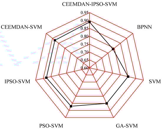
Figure 10.
Figure 10. Comparison results of the prediction effectiveness.
5.2. Grey Relational Analysis
To test the correlation degree between the prediction results of different methods and the actual data, the Grey relational degree (GRD) is introduced. The coincidence degree of prediction curves reflects the proximity of GRD to 1. It is known that high GRD values indicate an excellent prediction performance. The specific operation process is as follows [48].
The average values of GRD are listed in Figure 11. The GRD values of the seven models, BPNN, SVM, GA–SVM, PSO–SVM, IPSO–SVM, CEEMDAN–SVM, and CEEMDAN–IPSO–SVM, are 0.64, 0.68, 0.72, 0.74, 0.77, 0.74, and 0.80, respectively. It is found that the GRD values of the developed prediction model are higher than those of the comparison models, which proves the outstanding prediction performance of the developed prediction system.
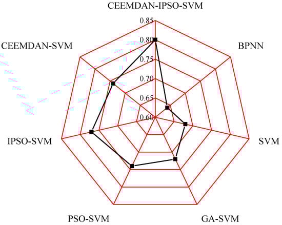
Figure 11.
Comparison results of the Grey relational degree.
5.3. Taylor Diagram
To better evaluate the performance of the established hybrid model, Taylor diagrams were used to compare the results [49]. Doing so provides a visualization of the models’ performances through standard deviations (SD), correlation coefficients, and RMSE. The diagram graphically represents the proposed models’ forecasting precision. The parameters evaluate the degree of agreement between the observed values and models.
In this paper, the proposed hybrid model is compared with BPNN, SVM, GA–SVM, PSO–SVM, IPSO–SVM, and CEEMDAN–SVM. A visualization of the models’ performances using Taylor diagrams is shown in Figure 12. The Taylor diagrams show that BPNN and SVM had a lower correlation and higher RMSE than the other models, and the standard deviation shows that the BPNN and SVM models deviated most from the observed values compared with other models. GA–SVM had a lower RMSE than the BPNN and SVM models, but it had the greatest standard deviation. PSO–SVM, IPSO–SVM, and CEEMDAN–SVM had higher correlation, lower RMSE, and better standard deviation. However, compared with the proposed model, the prediction effect can still be improved.
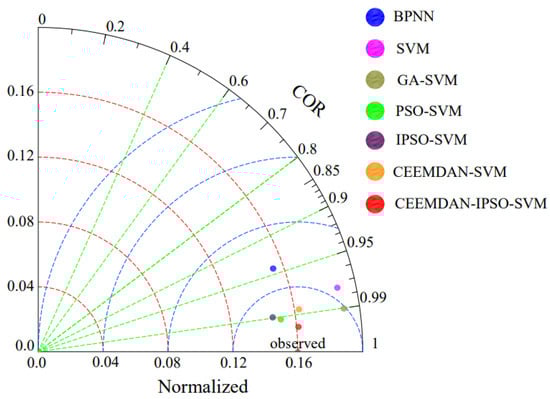
Figure 12.
Taylor diagram comparing model performance.
The CEEMDAN–IPSO–SVM model had a higher correlation and lower RMSE than the other models. The comparison of the standard deviations of the models showed that the CEEMDAN–IPSO–SVM model was more agreeable and closer to the observed values than the others.
6. Conclusions
- (1)
- To make the distribution rules of the training set and test set closer to the distribution rules of the original dataset, the stratified sampling method is applied in the division process. In the case of small samples, the large deviation caused by random sampling can be avoided, and the objectivity and reliability of the prediction results can be ensured.
- (2)
- The complete ensemble empirical mode decomposition with adaptive noise is proposed. By using the decomposition algorithm, the redundant noise in the prediction process can be eliminated, and the major features of the original datasets can be captured effectively.
- (3)
- To improve the exploration and exploitation capacities, eliminate the local optimal solutions, and avoid premature convergence, the improved particle swarm optimization method based on support vector regression is proposed. Through this method, the convergence rate and accuracy of the optimal solution are improved.
- (4)
- By combining the decomposition algorithm and the improved particle swarm optimization method based on support vector regression, a novel hybrid method for the corrosion rate prediction of natural gas pipelines is proposed. The evaluation module of this proposed model includes seven typical measurement rules, prediction effectiveness, Grey relational analysis, and the Taylor diagram. The outstanding performance and wide applicability of the proposed model are proved using natural gas pipelines. Taking the two dimensionless evaluation metrics of R2 and MAPE as examples, the proposed hybrid model can achieve prediction values of 0.925 and 5.73%, respectively, with the best prediction performance compared to conventional state-of-the-art models.
- (5)
- The proposed hybrid model can accurately predict the corrosion rate of natural gas pipelines; predict the possible corrosion accidents of pipelines in advance; guide the pipeline material selection, inhibitor filling process, and maintenance schedule; improve the corrosion control ability of pipelines; change the safety management measures of pipelines from post-processing to pre-event prevention; and provide decision support for the safe operation of pipelines.
Author Contributions
Conceptualization, L.X.; formal analysis, Z.Z.; funding acquisition, L.X.; investigation, J.Y.; methodology, J.Y.; resources, C.L.; software, L.X.; supervision, L.X., P.Y.; validation, Z.Z., C.L.; visualization, J.M., P.Y.; writing—original draft, L.X.; writing—review and editing, J.M., X.W., Y.Z. All authors have read and agreed to the published version of the manuscript.
Funding
This work was funded by the “Postdoctoral Research Program of PetroChina Southwest Oil & Gasfield Company” 20220305-18.
Institutional Review Board Statement
Not applicable.
Informed Consent Statement
Not applicable.
Data Availability Statement
Not applicable.
Conflicts of Interest
There are no conflict of interest to declare.
References
- Li, X.H.; Zhang, L.Y.; Khan, F.; Han, Z.Y. A data-driven corrosion prediction model to support digitization of subsea operations. Process Saf. Environ. Prot. 2021, 153, 413–421. [Google Scholar] [CrossRef]
- Soomro, A.A.; Mokhtar, A.A.; Kurnia, J.C.; Lashari, N.; Lu, H.M.; Sambo, C. Integrity assessment of corroded oil and gas pipelines using machine learning: A systematic review. Eng. Fail. Anal. 2022, 131, 105810. [Google Scholar] [CrossRef]
- Zhang, H.W.; Dong, S.H.; Ling, J.T.; Zhang, L.B.; Cheang, B. A modified method for the safety factor parameter: The use of big data to improve petroleum pipeline reliability assessment. Reliab. Eng. Syst. Saf. 2020, 198, 106892. [Google Scholar] [CrossRef]
- Cruz, J.P.B.; Veruz, E.G.; Aoki, I.V.; Schleder, A.M.; Souza, G.F.M.; Vaz, G.L.; Barros, L.O.; Orlowski, R.T.C.; Martins, M.R. Uniform corrosion assessment in oil and gas pipelines using corrosion prediction models—Part 1: Models performance and limitations for operational field cases. Process Saf. Environ. Prot. 2022, 167, 500–515. [Google Scholar] [CrossRef]
- Tang, Y.F.; Zhang, Q. Corrosion Control Technology and Practice in the Development of High Sulfur Gas Reservoirs; Petroleum Industry Press: Beijing, China, 2018. [Google Scholar]
- Kim, C.; Chen, L.; Wang, H.; Castaneda, H. Global and local parameters for characterizing and modeling external corrosion in underground coated steel pipelines: A review of critical factors. J. Pipeline Sci. Eng. 2021, 1, 17–35. [Google Scholar] [CrossRef]
- Xu, L.; Wang, Y.F.; Mo, L.; Tang, Y.F.; Wang, F.; Li, C.J. The research progress and prospect of data mining methods on corrosion prediction of oil and gas pipelines. Eng. Fail. Anal. 2023, 144, 106951. [Google Scholar] [CrossRef]
- Schneider, W.R. Corrosion Coupons and Pipe Life Predictions-Revision of 1947. Corrosion 1947, 3, 209–220. [Google Scholar] [CrossRef]
- Al-Fakih, A.M.; Algamal, Z.Y.; Lee, M.H. Quantitative structure-activity relationship model for prediction study of corrosion inhibition efficiency using two-stage sparse multiple linear regression. J. Chemom. 2016, 30, 361–368. [Google Scholar] [CrossRef]
- Du, J.Y.; Liao, K.X.; Li, C.J. Prediction the pitting depth growth in oil & gas pipelines with the times series analysis method. Xin Jiang Oil Gas 2005, 1, 80–82. [Google Scholar]
- Liu, Z.G.; Mu, Z.T. Research on Aircraft LY12CZ Aluminum Alloy Corrosion Damage Prediction Based on ARIMA Model. Adv. Mater. Res. 2011, 308–310, 1016–1022. [Google Scholar] [CrossRef]
- Tan, K.R.; Xiao, X. The forecast of remaining life of corrosive submarine pipelines based on grey theory. J. Shanghai Jiaotong Univ. 2007, 2, 186–188. [Google Scholar]
- Mekala, M.S.; Dhiman, G.; Viriyasitavat, W.; Park, J.H.; Jung, H.Y. Efficient LiDAR-Trajectory Affinity Model for Autonomous Vehicle Orchestration. IEEE Trans. Intell. Transp. Syst. 2023, 1–11. [Google Scholar] [CrossRef]
- Ma, H.N.; Zhang, W.D.; Wang, Y.; Ai, Y.B.; Zheng, W.Y. Advances in corrosion growth modeling for oil and gas pipelines: A review. Process Saf. Environ. Prot. 2023, 171, 71–86. [Google Scholar] [CrossRef]
- Singh, N.; Hamid, Y.; Juneja, S.; Srivastava, G.; Dhiman, G.; Gadekallu, T.R.; Shah, M.A. Load balancing and service discovery using Docker Swarm for microservice based big data applications. J. Cloud Comput. 2023, 12, 4. [Google Scholar] [CrossRef]
- Akhlaghi, B.; Mesghali, H.; Ehteshami, M.; Mohammadpour, J.; Salehi, F.; Abbassi, R. Predictive deep learning for pitting corrosion modeling in buried transmission pipelines. Process Saf. Environ. Prot. 2023, 174, 320–327. [Google Scholar] [CrossRef]
- Akbarzadeh, S.; Akbarzadeh, K.; Ramezanzadeh, M. Corroded resistance enhancement of sol-gel coating by incorporation of modified carbon nanotubes: Artificial neural network (ANN) modeling and experimental explorations. Prog. Org. Coat. 2023, 174, 107296. [Google Scholar] [CrossRef]
- Yang, D.D.; Hou, N.; Lu, J.Y.; Ji, D.A. Novel leakage detection by ensemble 1DCNN-VAPSO-SVM in oil and gas pipeline system. Appl. Soft Comput. 2022, 115, 108212. [Google Scholar] [CrossRef]
- Wang, C.; Han, F.; Zhang, Y.; Lu, J.Y. An SAE-based resampling SVM ensemble learning paradigm for pipeline leakage detection. Neurocomputing 2020, 403, 237–246. [Google Scholar] [CrossRef]
- Feng, J.P.; Gao, K.; Gao, W.; Liao, Y.C.; Wu, G. Machine learning-based bridge cable damage detection under stochastic effects of corrosion and fire. Eng. Struct. 2022, 264, 114421. [Google Scholar] [CrossRef]
- Peng, S.B.; Zhang, Z.; Liu, E.B.; Liu, W.; Qiao, W.B. A new hybrid algorithm model for prediction of internal corrosion rate of multiphase pipeline. J. Nat. Gas Sci. Eng. 2021, 85, 103716. [Google Scholar] [CrossRef]
- Manan, A.; Kamal, K.; Ratlamwala, T.A.H.; Sheikh, M.F.; Abro, A.G.; Zafar, T. Failure classification in natural gas pipe-lines using artificial intelligence: A case study. Energy Rep. 2021, 7, 7640–7647. [Google Scholar] [CrossRef]
- Duan, K.; Keerthi, S.S.; Poo, A.N. Evaluation of simple performance measures for tuning SVM hyperparameters. Neurocomputing 2003, 51, 41–59. [Google Scholar] [CrossRef]
- Seghier, M.E.A.B.; Keshtegar, B.; Tee, K.F.; Zayed, T.; Abbassi, R.; Trung, N.T. Prediction of maximum pitting corrosion depth in oil and gas pipelines. Eng. Fail. Anal. 2020, 112, 104505. [Google Scholar] [CrossRef]
- Wang, P.F.; Wang, S.X.; Ma, G. Prediction of internal corrosion rate of submarine multiphase flow pipelines based on PCA-PSO-SVM model. Saf. Environ. Eng. 2020, 27, 183–189. [Google Scholar]
- Jia, Z.G.; Ho, S.C.; Li, Y.; Kong, B.; Hou, Q.M. Multipoint hoop strain measurement based pipeline leakage localization with an optimized support vector regression approach. J. Loss Prev. Process Ind. 2019, 62, 103926. [Google Scholar] [CrossRef]
- Hatami, S.; Ardakani-Ghaderi, A.; Niknejad-Khomami, M.; Malekabadi, F.K.; Rassri, M.; Mohammadi, A.H. On the prediction of CO2 corrosion in petroleum industry. J. Supercrit. Fluids 2016, 117, 108–112. [Google Scholar] [CrossRef]
- Lu, H.F.; Iseley, T.; Matthews, J.; Liao, W.; Azimi, M. An ensemble model based on relevance vector machine and multi-objective salp swarm algorithm for predicting burst pressure of corroded pipelines. J. Pet. Sci. Eng. 2021, 203, 108585. [Google Scholar] [CrossRef]
- Liang, H.B.; Cheng, G.; Zhang, Z.D.; Yang, H. Research on ultrasonic defect identification method of well control manifold pipeline based on IAFSA-SVM. Measurement 2022, 194, 110854. [Google Scholar] [CrossRef]
- Li, J.; Du, C.W.; Liu, Z.Y. Effect of microstructure on the corrosion resistance of 2205 duplex stainless steel. Part 2: Electrochemical noise analysis of corrosion behaviors of different microstructures based on wavelet transform. Constr. Build. Mater. 2018, 189, 1294–1302. [Google Scholar] [CrossRef]
- May, Z.; Alam, M.K.; Nayan, N.A. Acoustic emission corrosion feature extraction and severity prediction using hybrid wavelet packet transform and linear support vector classifier. PLoS ONE 2021, 16, e0261040. [Google Scholar] [CrossRef]
- Li, Z.; He, T.L.; Tang, S.F. New corrosion rate prediction method for oil and gas pipelines based on EMD and modified GM (1,N) model. Hot Work. Technol. 2023, 52, 35–42. [Google Scholar]
- Ning, F.L.; Cheng, Z.H.; Meng, D.; Wei, J. A framework combining acoustic features extraction method and random forest algorithm for gas pipeline leak detection and classification. Appl. Acoust. 2021, 182, 108255. [Google Scholar] [CrossRef]
- Huang, N.E.; Shen, Z.; Long, S.R.; Wu, M.C.; Shih, H.H.; Zheng, Q.; Yen, N.C.; Liu, H.H. The empirical mode decomposition and the Hilbert spectrum for nonlinear and non-stationary time series analysis. Proc. Math. Phys. Eng. Sci. 1998, 454, 903–995. [Google Scholar] [CrossRef]
- Wu, Z.; Huang, N.E. Ensemble empirical mode decomposition: A noise-assisted data analysis method. Adv Adapt. Data Anal 2009, 1, 1–41. [Google Scholar] [CrossRef]
- Torres, M.E.; Colominas, M.A.; Schlotthauer, G.; Flandrin, P. A complete ensemble empirical mode decomposition with adaptive noise. In Proceedings of the 2011 IEEE International Conference on Acoustics, Speech and Signal Processing (ICASSP), Prague, Czech Republic, 22–27 May 2011. [Google Scholar]
- Kennedy, J.; Eberhart, R. Particle swarm optimization. Proc. IEEE Int. Conf. Neural Netw. 1995, 4, 1942–1948. [Google Scholar]
- Vapnik, V. The Nature of Statistical Learning Theory; Springer: NewYork, NY, USA, 1995. [Google Scholar]
- Shawe-Taylor, J.; Bartlett, P.L.; Williamson, R.C.; Anthony, M. Structural risk minimization over data-dependent hierarchies. IEEE Trans. Inf. Theory 1998, 44, 1926–1940. [Google Scholar] [CrossRef]
- Janik, P.; Lobos, T. Automated Classification of Power-Quality Disturbances Using SVM and RBF Networks. IEEE Trans. Power Deliv. 2006, 21, 1663–1669. [Google Scholar] [CrossRef]
- Guo, H.; Yin, J.; Zhao, J. Prediction of fatigue life of packaging EMC material based on RBF-SVM. Int. J. Mater. Prod. Technol. 2014, 49, 5–17. [Google Scholar] [CrossRef]
- Hens, A.B.; Tiwari, M.K. Computational time reduction for credit scoring: An integrated approach based on support vector machine and stratified sampling method. Expert Syst. Appl. 2012, 39, 6774–6781. [Google Scholar] [CrossRef]
- Ye, Y.M.; Wu, Q.Y.; Huang, J.Z.; Ng, M.K.; Li, X.T. Stratified sampling for feature subspace selection in random forests for high dimensional data. Pattern Recognit. 2013, 46, 769–787. [Google Scholar] [CrossRef]
- Li, X.H.; Jia, R.C.; Zhang, R.R.; Yang, S.Y.; Chen, G.M. A KPCA-BRANN based data-driven approach to model corrosion degradation of subsea oil pipelines. Reliab. Eng. Syst. Saf. 2022, 219, 108231. [Google Scholar] [CrossRef]
- Wang, Q.Y.; Song, Y.H.; Zhang, X.S.; Dong, L.J.; Xi, Y.C.; Zeng, D.Z.; Liu, Q.L.; Zhang, H.L.; Zhang, Z.; Yan, R.; et al. Evolution of corrosion prediction models for oil and gas pipelines: From empirical-driven to data-driven. Eng. Fail. Anal. 2023, 146, 107097. [Google Scholar] [CrossRef]
- Zhi, Y.J.; Jin, Z.H.; Lu, L.; Yang, T.; Zhou, D.Y.; Pei, Z.B.; Wu, D.Q.; Fu, D.M.; Zhang, D.W.; Li, X.G. Improving atmospheric corrosion prediction through key environmental factor identification by random forest-based model. Corros. Sci. 2021, 178, 109084. [Google Scholar] [CrossRef]
- Chen, H.; Hou, D. Research on superior combination forecasting model based on forecasting effective measure. J. Univ. Sci. Technol. China 2002, 2, 172–180. [Google Scholar]
- Wu, H.Y.; Lei, H.G.; Chen, Y. Grey relational analysis of static tensile properties of structural steel subjected to urban industrial atmospheric corrosion and accelerated corrosion. Constr. Build. Mater. 2022, 315, 125706. [Google Scholar] [CrossRef]
- Taylor, K.E. Summarizing multiple aspects of model performance in a single diagram. J. Geophys. Res. 2001, 106, 7183–7192. [Google Scholar] [CrossRef]


Disclaimer/Publisher’s Note: The statements, opinions and data contained in all publications are solely those of the individual author(s) and contributor(s) and not of MDPI and/or the editor(s). MDPI and/or the editor(s) disclaim responsibility for any injury to people or property resulting from any ideas, methods, instructions or products referred to in the content. |
© 2023 by the authors. Licensee MDPI, Basel, Switzerland. This article is an open access article distributed under the terms and conditions of the Creative Commons Attribution (CC BY) license (https://creativecommons.org/licenses/by/4.0/).