Article

Mike 21 Model Based Numerical Simulation of the Operation Optimization Scheme of Sedimentation Basin

1
School of Water Conservancy, North China University of Water Resources and Electric Power, Zhengzhou 450046, China
2
Key Laboratory of Lower Yellow River Channel and Estuary Regulation, MWR, Yellow River Institute of Hydraulic Research, YRCC, Zhengzhou 450003, China
3
Water Development Planning and Construction Co., Ltd., Jinan 250000, China
4
State Key Laboratory of Simulation and Regulation of Water Cycle in River Basin, China Institute of Water Resources and Hydropower Research, Beijing 100046, China
5
Hubei Key Laboratory of Disaster Prevention and Mitigation, China Three Gorges University, Wuhan 443002, China
6
School of Civil Engineering, Henan Polytechnic University, Jiaozuo 454000, China
*
Author to whom correspondence should be addressed.
Coatings 2022, 12(4), 478; https://doi.org/10.3390/coatings12040478
Submission received: 22 February 2022 / Revised: 27 March 2022 / Accepted: 30 March 2022 / Published: 1 April 2022
(This article belongs to the Special Issue Energy, Material Science and Environmental Engineering)

Abstract

:
The sedimentation basin is an important part of hydraulic engineering. Because the prototype size is too large and not easy to analyze, Mike 21 has the advantages of easy input, conversion, analysis, and demonstration of data results, which are flexible and convenient; however, this method has not been used in hydraulic engineering by previous researchers. This research used the sedimentation basin of the Yellow River Diversion Project as the research object, and a simulation model of the sedimentation basin channel #1 was developed using Mike 21 software to analyze its water and sediment characteristics and conditions in different periods. Using numerical simulation methods, three types of sedimentation basin operation schemes were targeted, the sedimentation changes and sedimentation law of channel #1 were evaluated in each scheme, and the sedimentation effects were compared. The results show that in conditions of different incoming water and sediment and diversion timings during the flood and non-flood seasons, the sedimentation basin adopts an operation scheme to lower the outlet water level, and the siltation volumes are 180,000 and 150,000 m3 lower than the high-outlet water levels, respectively. Moreover, its siltation status is significantly improved, which can effectively extend the service life of the sedimentation basin, prolong the period of silting removal by about 3.5 months, and provide a scientific basis and reference for the optimization of the operation mode of the sedimentation basin in other types of hydraulic engineering.

1. Introduction

The treatment of sediment in sediment-laden flow based on the utilization of a sedimentation basin is an effective measure in hydraulic engineering. The working principle of the sedimentation basin is that the flow velocity of sediment-laden water decreases upon entering the sedimentation basin. This reduces the sediment-carrying capacity of the current and changes the original movement state of the sediment to achieve sedimentation [1]. Sedimentation basins are an indispensable part of the Yellow River Diversion Project. Currently, the silt in the early stage of the sedimentation basin is very serious, and there exist problems such as the poor effect of settling. Although the first dredging was completed in May 2021, the cumulative dredging was approximately 3 million m3; however, the operation mode of the sedimentation basin did not change. To improve sedimentation, the issue of the utilization of sand ponds ought to be addressed. Moreover, arable land resources were destroyed during the dredging process and caused ecological and environmental problems such as soil salinization and desertification. To improve the use of sedimentation basins and improve the ecological environment, scholars at home and abroad have explored the characteristics of water and sand movement, model construction, and optimization of the sedimentation basin.
Bagnold [2] derived the calculation formulas for the bedload and suspended load sediment transport rate, which promoted the development of sediment research. Zee C.H. and R [3] introduced new formulas for the transportation of bedload. Chen et al. [4] analyzed the sequence of annual runoff and sediment and clarified the influence of hydraulic engineering on the downstream runoff deposition relationship, which gradually weakened from upstream to downstream. An et al. [5] systematically analyzed the water and sediment data of the Ningmeng River section of the Yellow River since the 1960s and determined that the sediments of the river channel were mainly composed of the mainstream and tributary. Krishnappan et al. [6] studied the variation rule of sediment particle size and settling speed during the process of sediment settling and showed that smaller particle sizes fell and silted more easily. Asgharzadeh et al. [7] assessed the influence of baffle length on particle settlement in a rectangular sedimentation basin. Bürger et al. [8] proposed a one-dimensional model for the continuous sedimentation process in a settling basin with a variable cross-sectional area. Wang and Fu [9] studied the flow characteristics of an inclined-tube sedimentation basin used to separate water and sediment in the Yellow River. The movement and flow characteristics in the sedimentation basin were determined using computer-aided visualization. The performance of an inclined-improved conventional up-flow settling basin was studied by Saady [10].
Based on the computational fluid dynamics (CFD) model, Shahrokhi et al. [11] re-searched the best position of a baffle in a rectangular, primary sedimentation basin. Kim et al. [12] analyzed the influences of the length and position of the baffle at the entrance of a circular sedimentation basin on the settlement of suspended solids. Tarpagkou and Pantokratoras [13] and Liu et al. [14] simulated sedimentation basins with different particle sizes and volume fractions using numerical simulations. Razmia et al. [15] calculated the flow field and flow curve of the initial flow rate in a sedimentation basin. Tarpagkou and Pantokratoras [16] also simulated the dynamic flow structure of a rectangular sedimentation basin for potable water using a multiphase method. Using the k–ε turbulence model, Sammarraee et al. [17] studied the flow and sediment movement law of a bar sedimentation basin, and Liu et al. [18,19] simulated the influence of baffles on the hydraulic characteristics of a sedimentation basin. The sediment movement characteristics of the sedimentation basin were simulated and analyzed by Olsen and Kjellesvig [20] and Jayanti and Narayanan [21]. Bajcar et al. [22,23] studied the influence of the flow field on the settling efficiency of sedimentation basins. Stamou et al. [24] and Ramin et al. [25] analyzed the sediment settling law of a sedimentation basin.
The water flow in the sedimentation basin was affected considerably by the baffle, which could improve the performance of the sedimentation basin and reduce the influence of adverse phenomena [26]. Saeedi et al. [27] proposed a method to change the geometry of the baffle installed at the bottom part of the sedimentation basin to improve the settling efficiency of the rectangular sedimentation basin and determine the optimal geometry of the baffle. Guo et al. [28] successively applied continuity and momentum equations to solve solid–fluid motion using the finite element method and studied the removal of fine particles in a three-stage sedimentation basin with an adjustable baffle. Vhidifar et al. [29] used Fluent to study a full-size rectangular sedimentation basin and proposed three additional baffle methods to optimize the sedimentation basin. In addition, Gupta [30] established a curve related to the efficiency of a sedimentation basin. Tarpagkou and Pantokratoras [13] studied the influence of different sediment concentrations on the flow field in a sedimentation basin and selected the appropriate operation mode according to the conditions of different sediment concentrations.
Previous studies have conducted in-depth research on the characteristics of water and sand movements in sedimentation basins. However, the final CFD results cannot provide any form of analytical expressions but only a numerical solution on a limited number of discrete points. Additionally, there are certain calculation errors, and by adjusting the baffle to optimize the sedimentation basin, it is only suitable for small-size sedimentation basins and not suitable for hydraulic engineering. Considering this, the software Mike 21 was used owing to its advantages, including easy data input, data conversion and analysis, and the presentation of the results, which makes it quite flexible and convenient.
The research object of this study was the sedimentation basin of the Yellow River Diversion Project, and the study combined its water and sediment characteristics and incoming water and sediment conditions in different periods, divided the channel #1 mesh of the sedimentation basin using SMS software, preprocessed it, and imported the obtained channel #1 mesh file in Mike 21. This research used the hydrodynamic module and sediment transport module in Mike 21 to simulate the evolution process of sedimentation, excavated the law of sedimentation, proposed different optimization schemes, compared the changes in sediment content and sedimentation conditions of the sedimentation basin in different schemes, and determined the optimal sedimentation effect scheme.

2. Materials and Methods
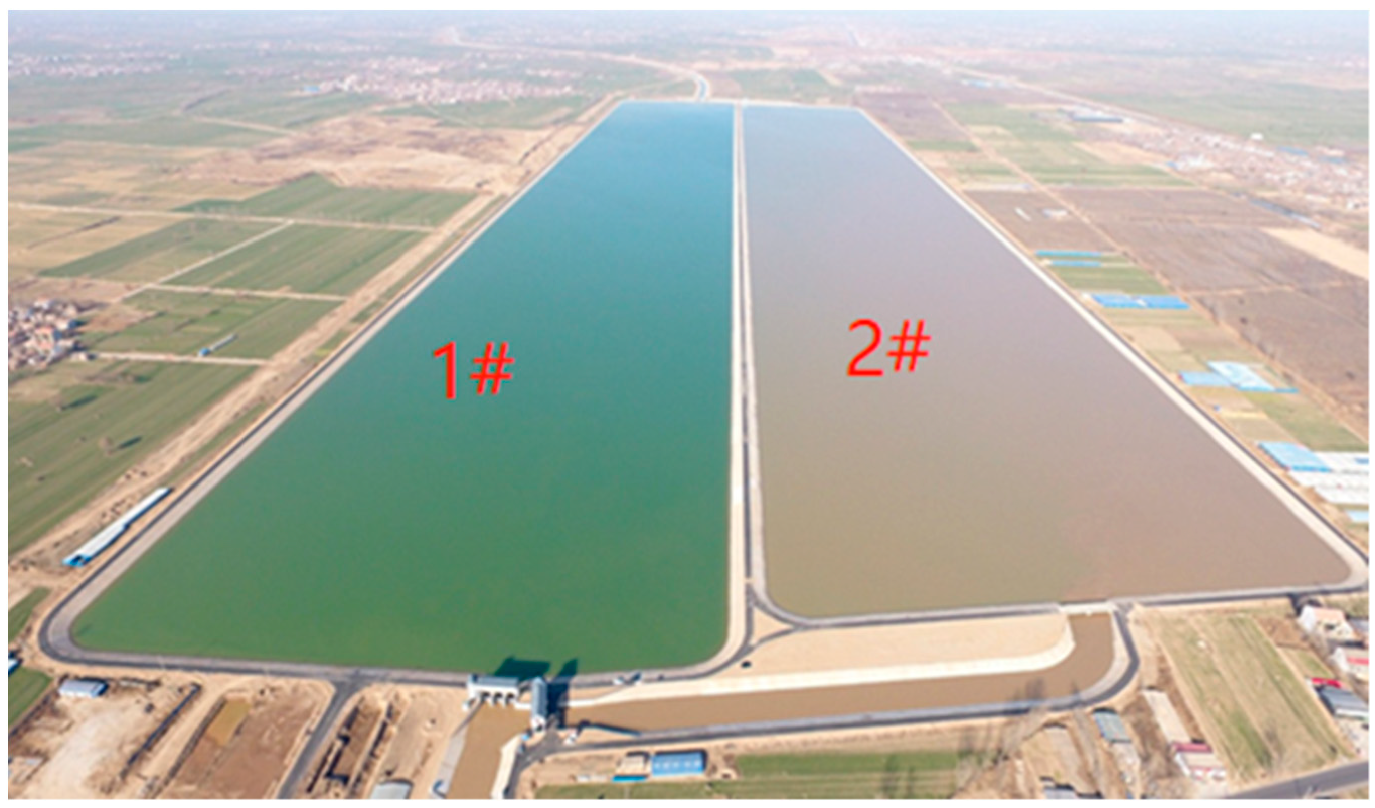
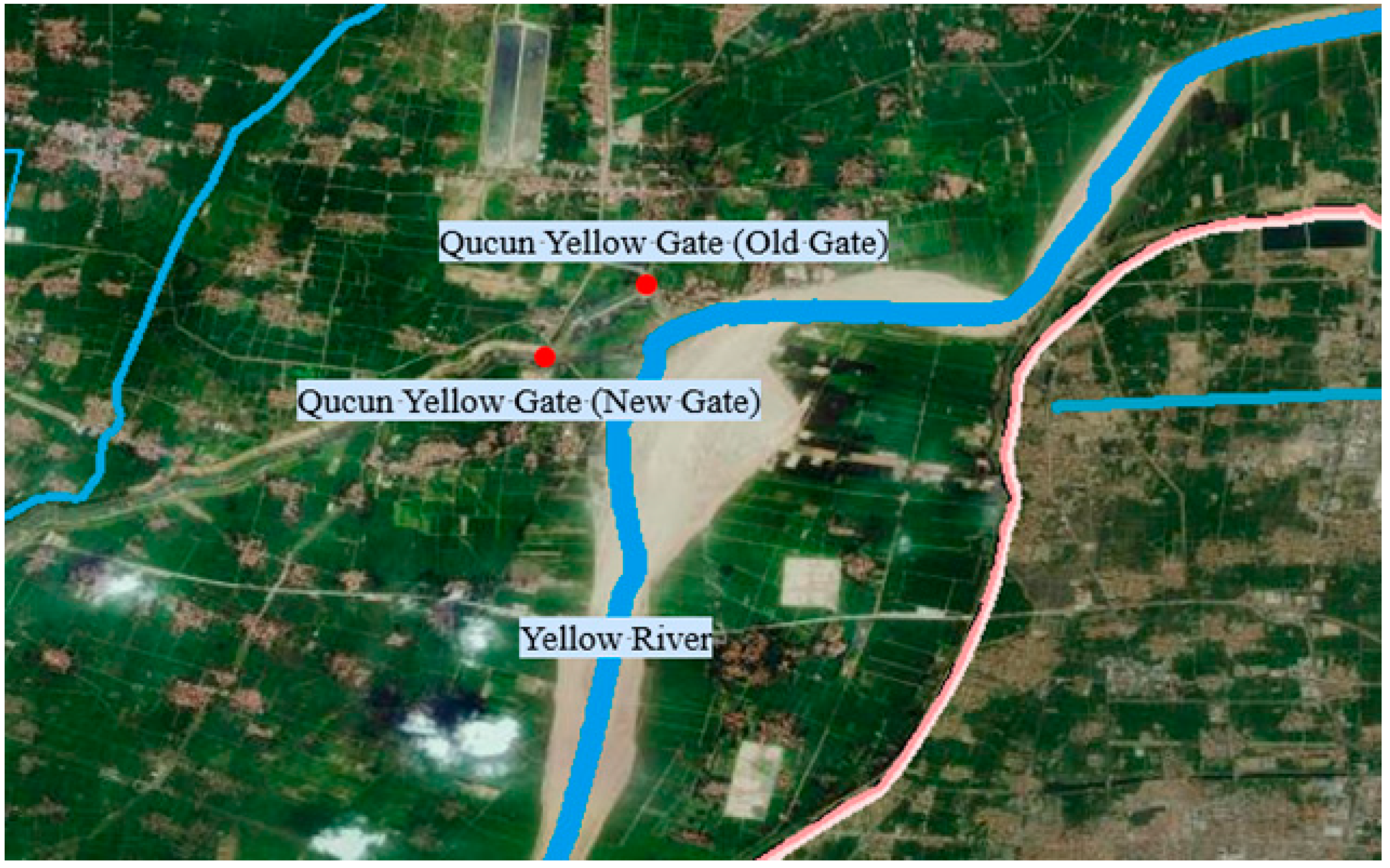
2.1. Study Area

The Yellow River Diversion Project is a major project implemented to ensure the eco-logical water supply for Xiongan, Baiyangdian, and the people along the route. The project was completed in 2018, and it diverted water from the Xin and Laoqucun sluices in Qucun and Laoqucun, Puyang City, Henan Province. The average water diversion volume from the Yellow River in Hebei Province for many years has been 620 million m3 (the water diversion period is winter and April). After the water delivery line from the Yellow River to Jibudian uses the main channel of Nanhu Lake in Puyang, Henan Province, it flows along the third south main channel of Puqing to the northwest via the Weihe inverted siphon to Hebei Province. It uses the existing rivers and ditches of Hebei Province to transport water automatically and finally into Baiyangdian. The sand basin is 2500 m long from north to south and 900 m wide from east to west. It covers an area of approximately 175 ha, as shown in Figure 1. It adopts a double channel design, with channel #1 on the left and channel #2 on the right, as shown in Figure 2. Partition and surrounding embankments were set between the two channels. The depth of the basin is approximately 4.5 m, and the elevation of its bottom part is in the range of 52.4–53.18 m.

2.2. Research Methods

In this research, SMS software was used to preprocess the channel #1 topographic data of the sedimentation basin, and mesh files of channel #1 were imported in Mike 21. The hydrodynamic module and sediment transport module in Mike 21 were used to analyze the water and sediment characteristics, in which the sediment module is a mathematical calculation based on the hydrodynamic module.

2.2.1. Model Principle

  • Hydrodynamic module principle
The FM module in Mike 21 was used in the hydrodynamic module, whereby the continuity equation of water flow is
h t + h u ¯ x + h v ¯ y = h S
The momentum equation in the X direction is
h u ¯ t + h u 2 ¯ x + h v u 2 ¯ y = f v h ¯ g h η x h ρ 0 p a x g h 2 ρ 2 ρ 0 x + τ s x ρ 0 1 ρ 0 ( S x x x + S x y x ) + x ( h T x x ) + x ( h T x y ) + h u s S
The momentum equation in the Y direction is
h v ¯ t + h u v ¯ x + h v 2 ¯ y = f u ¯ h g h η y h ρ 0 p a y g h 2 ρ 2 ρ 0 y + τ s x ρ 0 τ b y ρ 0 1 ρ 0 ( S y x y + S y y x ) + x ( h T x y ) + y ( h T y y ) + h v s S
where h = η + d is the total water depth, η is the water level, d is the static water depth, t is time, x and y are the Cartesian coordinates, u and v are the velocity components in the x and y directions, respectively, u ¯ and v ¯ are the average velocities of water depth, g is gravity acceleration, f is the coefficient of the Coriolis force term, f u ¯ and f v ¯ are accelerations caused by the rotation of the Earth, P a is the air pressure, ρ 0   is the normal seawater density, ρ is the density of water, S x x , S x y , S y x , S y y are the wave radiation stress terms, T x x , T x y , T y y are the horizontal viscous stress terms, S is the source and sink item, and u s   and   v s are the flow rates of the head and sink flows.
  • Sediment transport module principle
Control equation of sediment transport model:
c ¯ t + u c ¯ x + c ¯ y = 1 h x ( h D x c ¯ x ) + 1 h y ( h D y c ¯ y ) + Q L C L 1 h S
where c ¯ is the average sediment concentration in the water depth direction (kg/m3), h is the water depth (m), D x and D y are the dispersion coefficients in the x and y directions, respectively (m2/s), Q L is the single wide source term flow in the horizontal direction (m3/s/m3), C L is the source sediment concentration, g/m3, and S is the scouring/silting item kg/m3/s.
The settling speed adopts the Stokes settling speed formula:
ω = ( ρ s ρ ) g d 2 18 ρ v
where ω is the sedimentation velocity (m/s), ρ s is the bulk density of the sediment (kg/m3), ρ is the bulk density of water, kg/m3, g is the acceleration of gravity (m/s2), d is the sediment particle size (m), and ν is the kinematic viscosity coefficient of the water flow (m2/s).

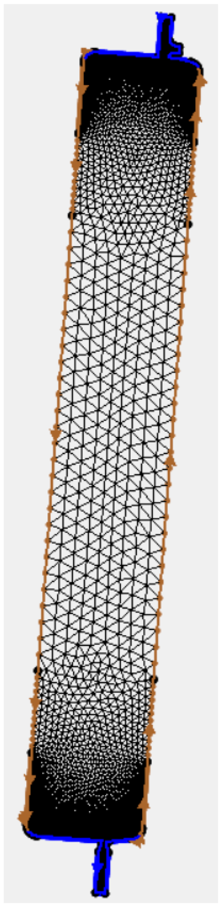
2.2.2. Model Establishment and Parameter Calibration

  • Model establishment
The topographic data of channel #1 in the sedimentation basin were preprocessed by the software SMS. After repeated debugging, the boundary attributes were defined as open and land boundaries. The distance 250 m from the entrance and exit was determined as a grid edge length equal to 5 m, and the distance in the range of 250–500 m from the entry and exit was divided by a grid edge length of 20 m. The middle part of the channel in the sedimentation basin was divided into 34,404 unstructured triangular grid units, as shown in Figure 3.
The mesh file for grid division of channel #1 in the sedimentation basin was imported in Mike 21, and the channel #1 model of the sedimentation basin was established. The elevation was based on the 1985 China elevation datum, the plane coordinate was based on the 1954 Beijing coordinate system, the height of the bottom part of the sedimentation basin was in the range of 52.4–53.18 m, the horizontal coordinate was 590,068 m, and the longitudinal coordinate was in the range of 399,000–3,921,500 m.
  • Parameter calibration
The parameters in hydrodynamic module are set using low-level operations; the drying depth is 0.005 m, the flooding depth is 0.05 m, the wetting depth is 0.1 m, and the eddy viscosity coefficient is 0.28; the river bed roughness is Manning coefficient calculation, set as 32 m1/3/s; initial water level is 53.5 m.
The parameters in sediment module: the sedimentation velocity of suspended sediment is selected as flocculation sedimentation, the flocculation condition is 0.01 kg/m3, and the density of sediment is 2650 kg/m3; for the distribution of suspended sediment in the water body, the critical siltation shear stress is 0.15 N/m2. Set up 1 sediment component and 2 bottom beds; bed 1 is soft mud layer, and bed 2 is hard mud layer. The scour coefficient of the first layer is 0.00005 kg/m2/s and the second layer is 1 kg/m2/s, while the density of the first bed is 200 kg/m3, and the density of the second bed is 400 kg/m3, given an initial concentration of component 1 of 0.001 kg/m3.

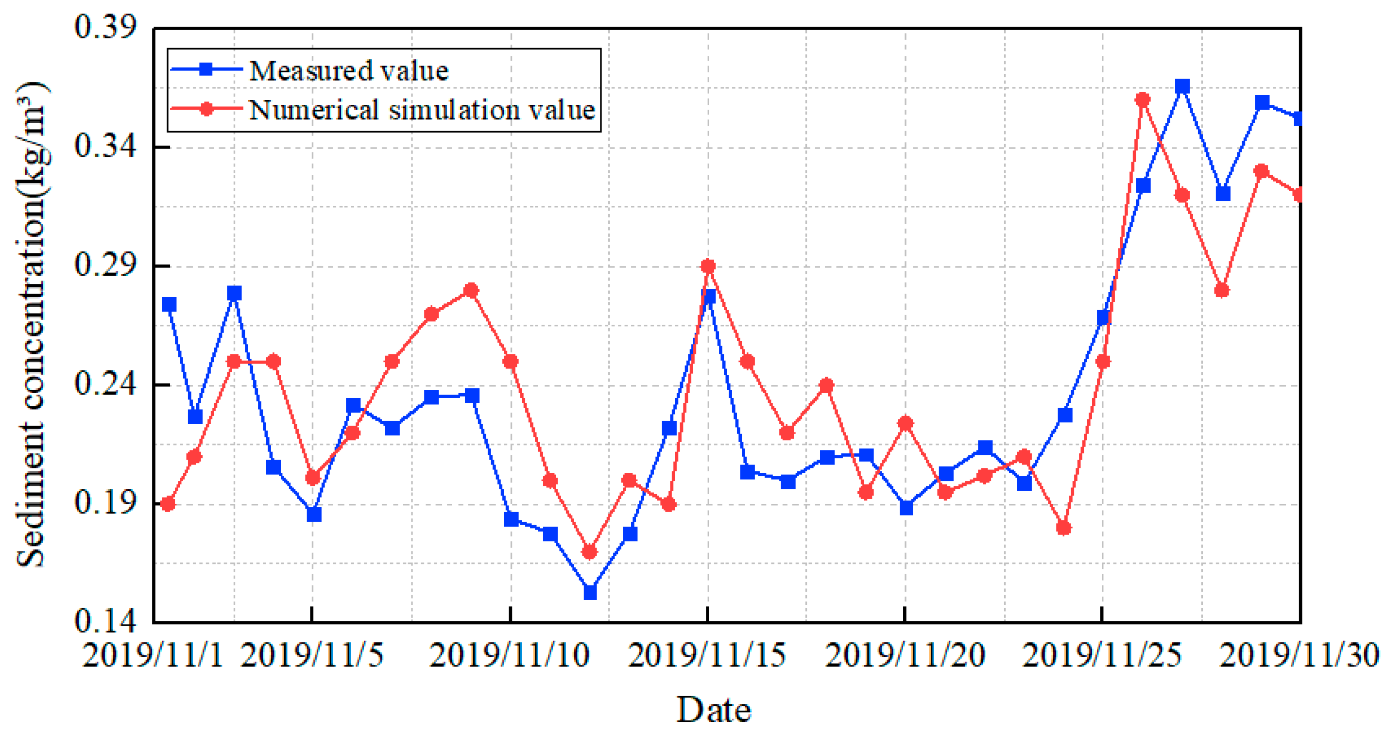
2.2.3. Model Validation

The sediment concentration at the outlet of the sedimentation basin in October 2019 was verified. The water level of the lower-boundary condition in the hydrodynamic module of Mike 21 was set at 56 m. Figure 3 shows the data changes needed to prove the effect of actual and simulated sediment concentration. Figure 4 shows that the fitting error between the simulated and measured sediment concentration values of the measuring station was <0.084 kg/m3. The two processes were consistent, and the fitting effect was perfect. Therefore, it was feasible to conduct this research using a calibrated model.

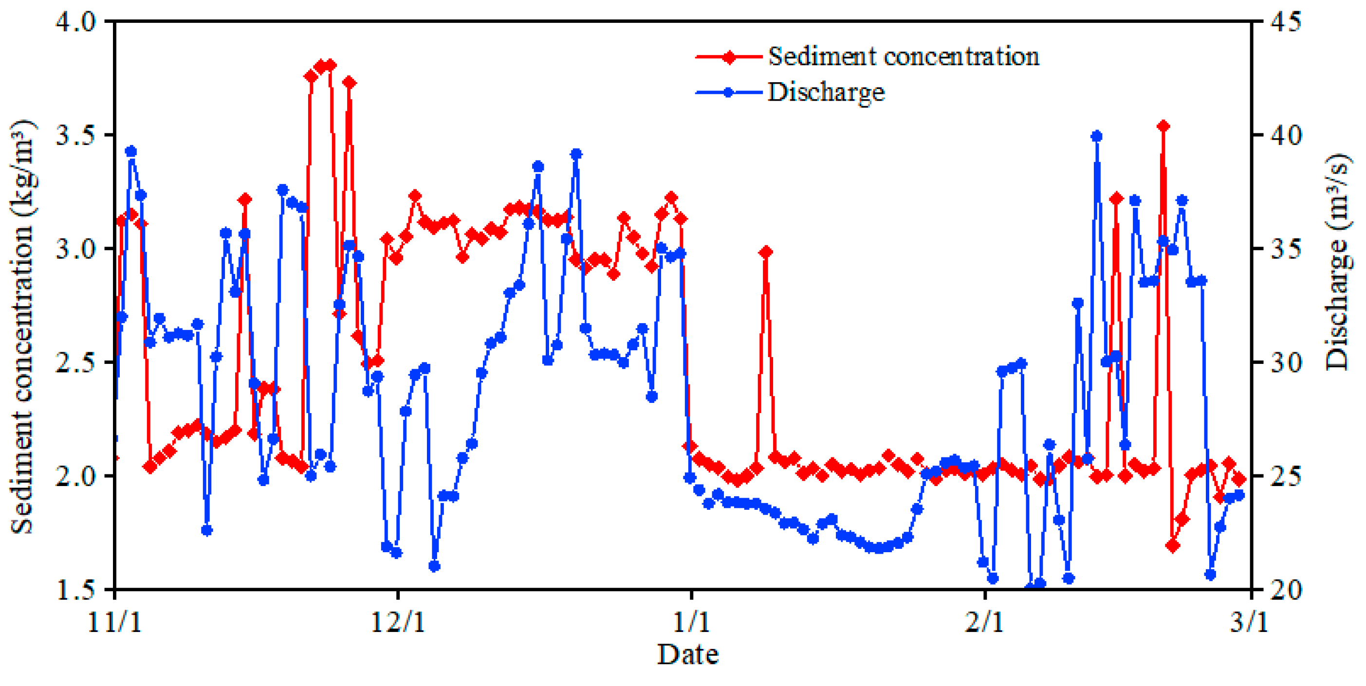
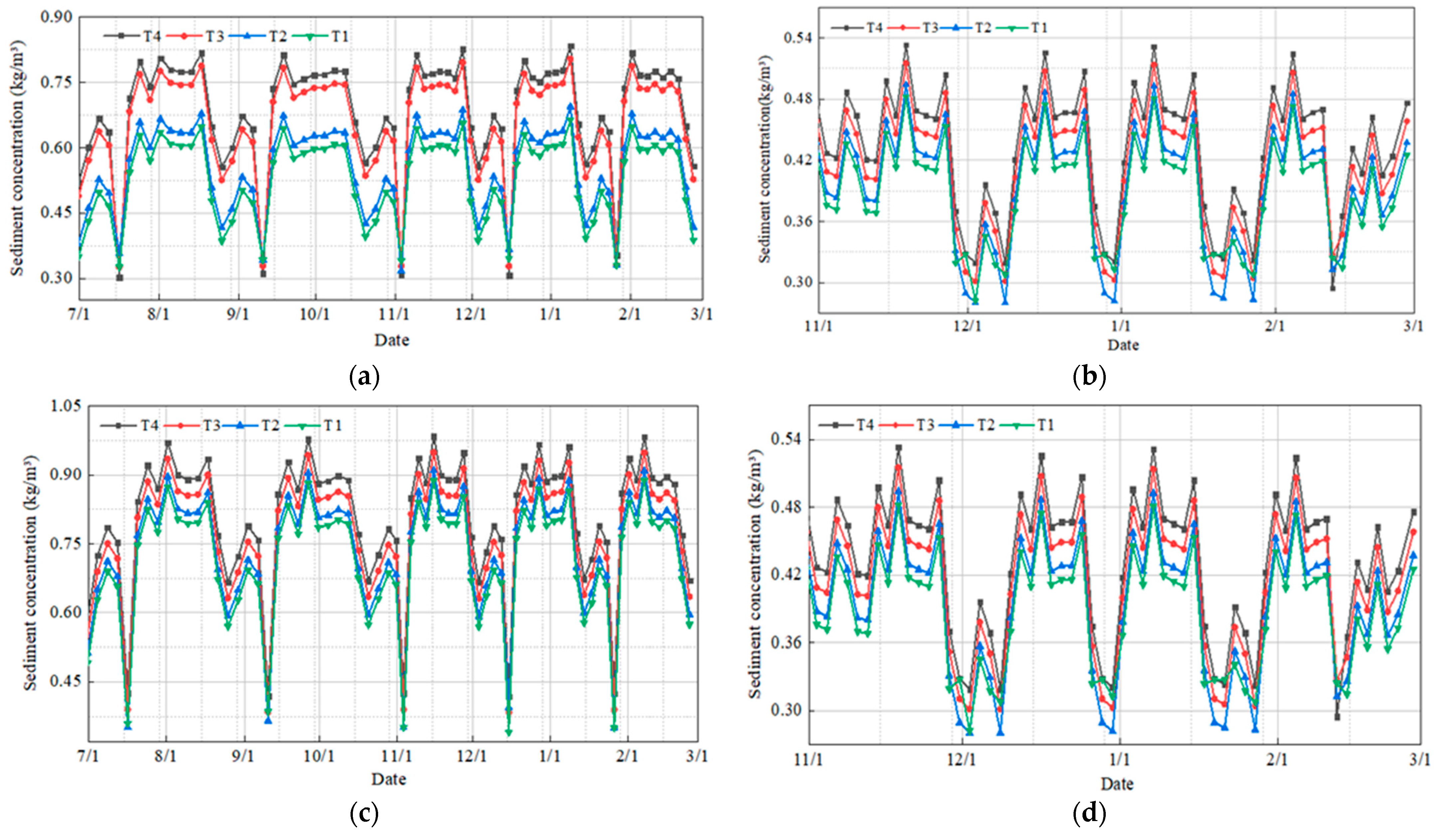
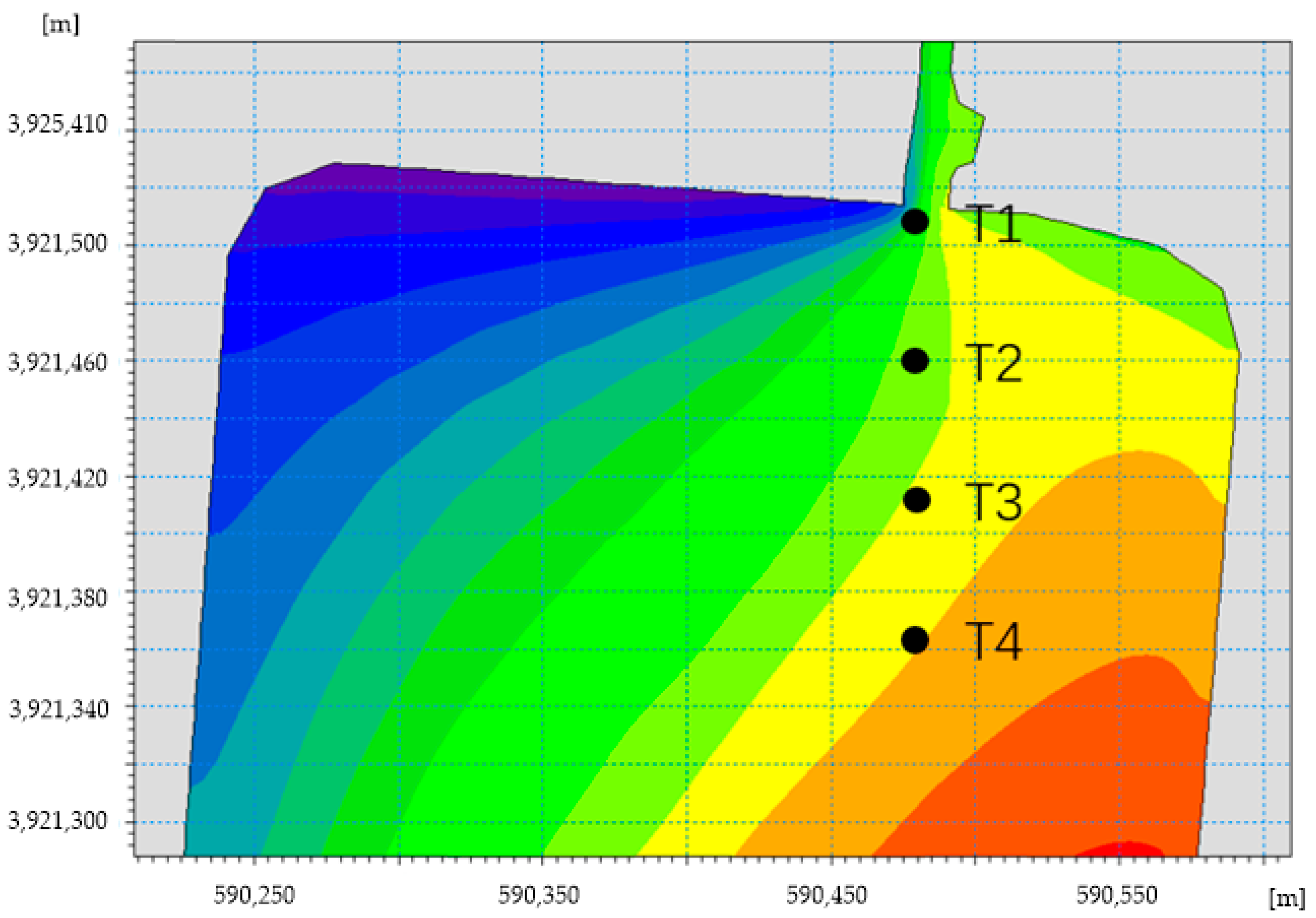
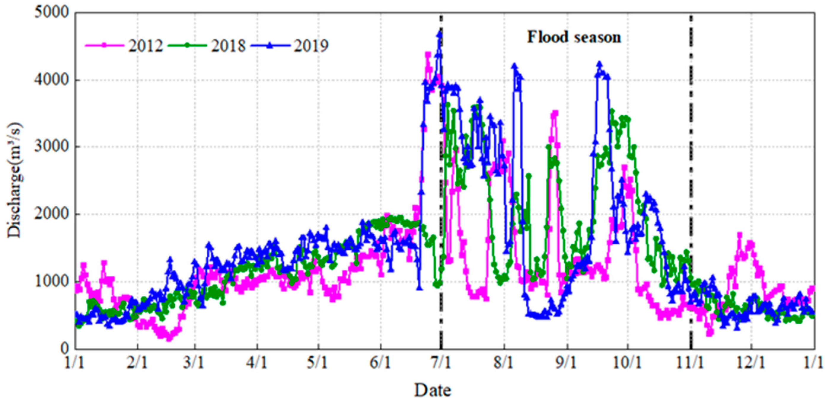
2.3. Analysis of Water and Sediment Characteristics

Based on the measured water diversion flow and sediment concentration in 2019, channel #1 model of the sedimentation basin was established with the use of Mike 21. The upper-boundary condition in the hydrodynamic model was set as a flow process, and the lower-boundary condition was set as a water level process. The upper-boundary condition in the sediment module was set as a sediment concentration process, and the lower-boundary condition was set as a zero-gradient boundary.

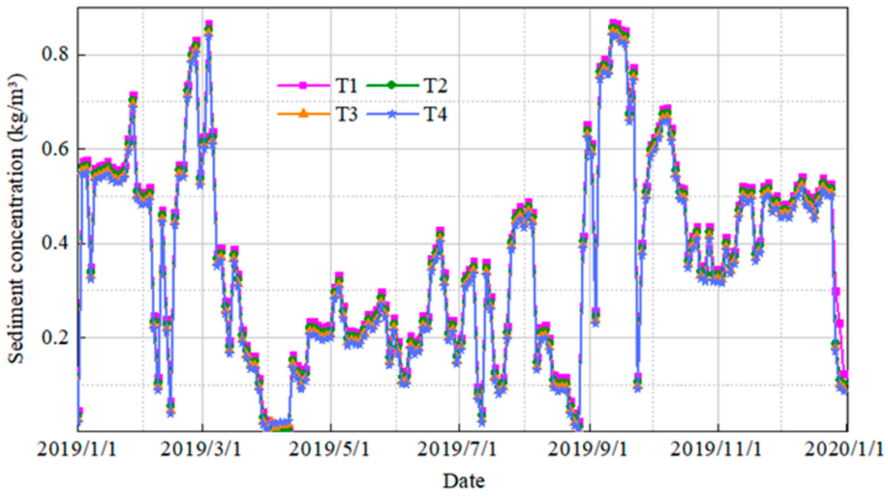
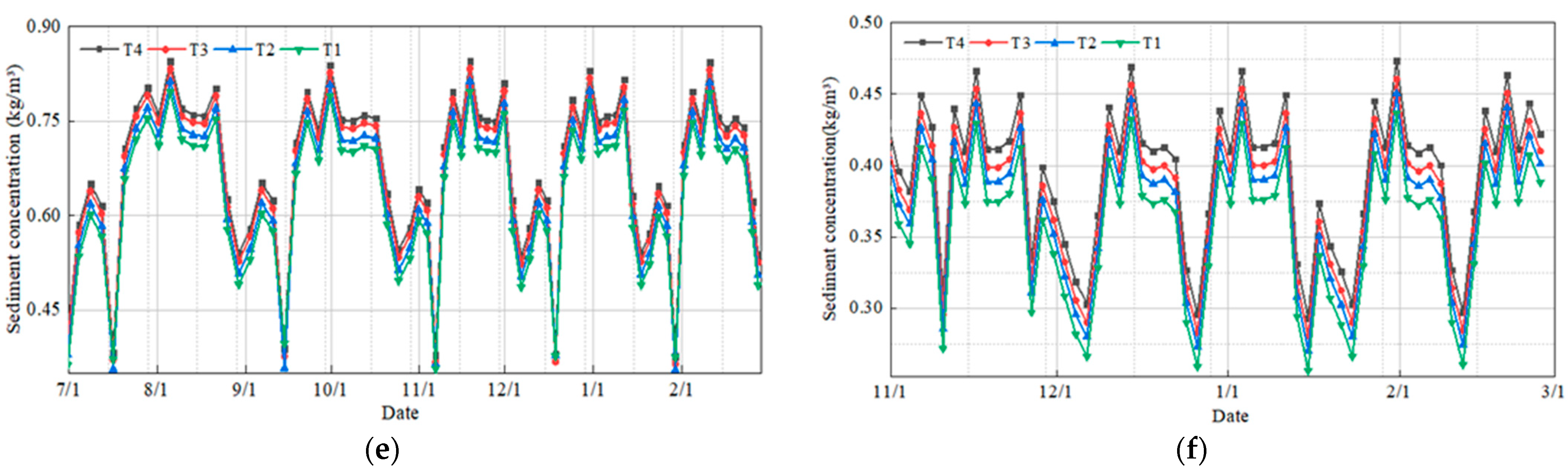
2.3.1. Sediment Content Analysis

The sediment content of channel #1 in the sedimentation basin yielded a maximum at the entrance and gradually decreased downstream. It progressively increased as the transverse coordinate increased such that the contents of the right middle and upper reaches were more extensive. With the increase in the longitudinal coordinates, the contents of the middle and upper reaches were significantly higher than those of the downstream sediment. The four characteristic points T1, T2, T3, and T4 were selected at the outlets of the sedimentation basin, and the coordinate range was (590,210, 3,921,290)~(590,610, 3,921,560), as shown in Figure 5.
The sediment concentration in the basin was 4.99 kg/m3, and that in the outlet was in the range of 1.16–1.22 kg/m3. The outlet diameter was <0.05 mm. Figure 6 shows the variation rule of the sediment concentration at the characteristic point. The figure shows that the variation trends of the sediment concentration at the expected points T1–T4 are the same, the maximum sediment concentration at the outlet is 0.85 kg/m3, and the minimum sediment concentration is 0.03 kg/m3. The daily average sediment concentrations at the characteristic points T1–T4 gradually decrease during the course and are equal to 0.34 kg/m3, 0.37 kg/m3, 0.38 kg/m3, and 0.39 kg/m3, respectively. This is significantly below the design requirements of the outlet basin.
In future water diversion processes, it can be considered to increase the sand content of the outlet and reduce the amount of siltation in the sedimentation basin to ensure the safety of the water diversion for improving the sedimentation effect.

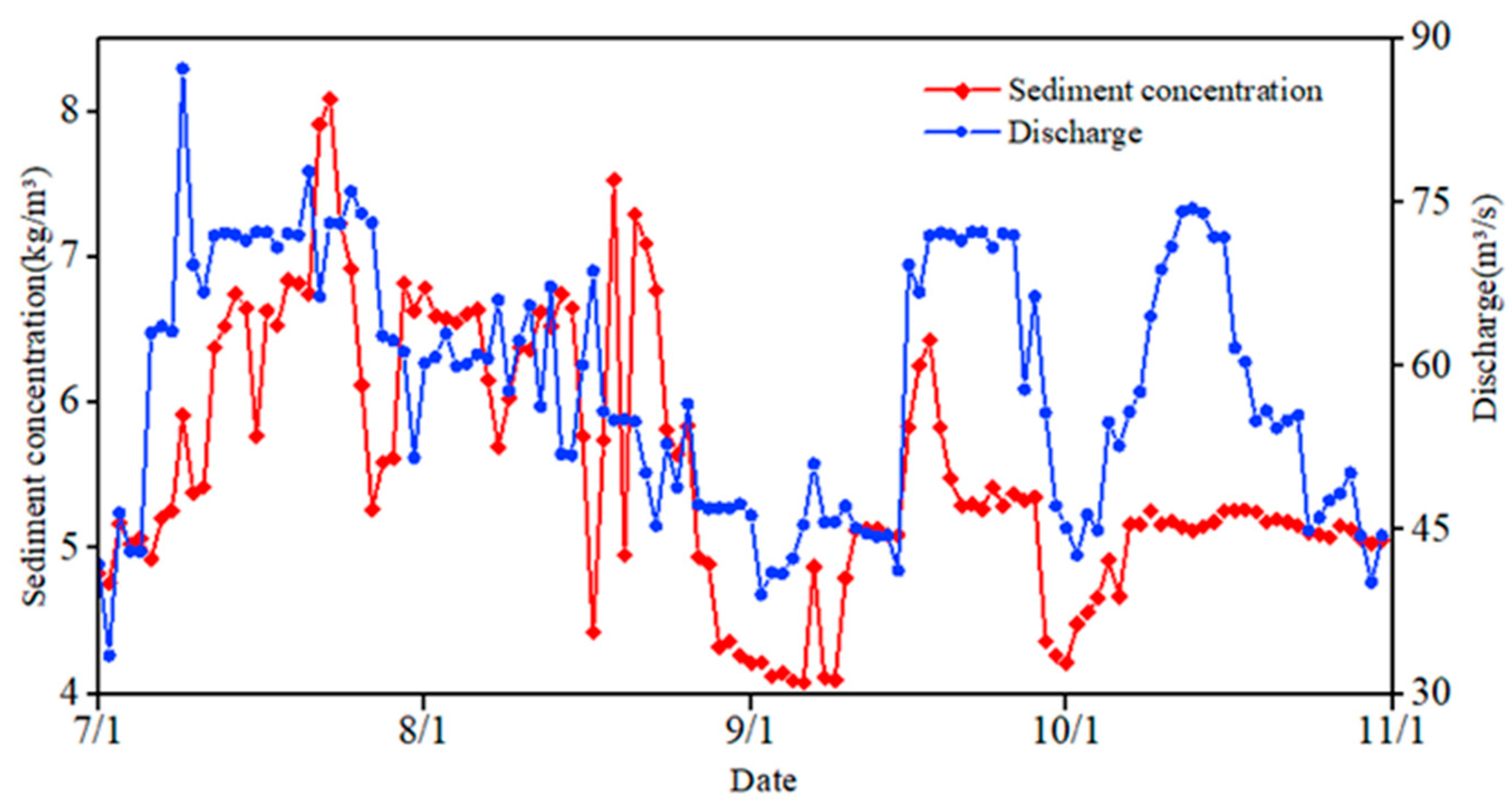
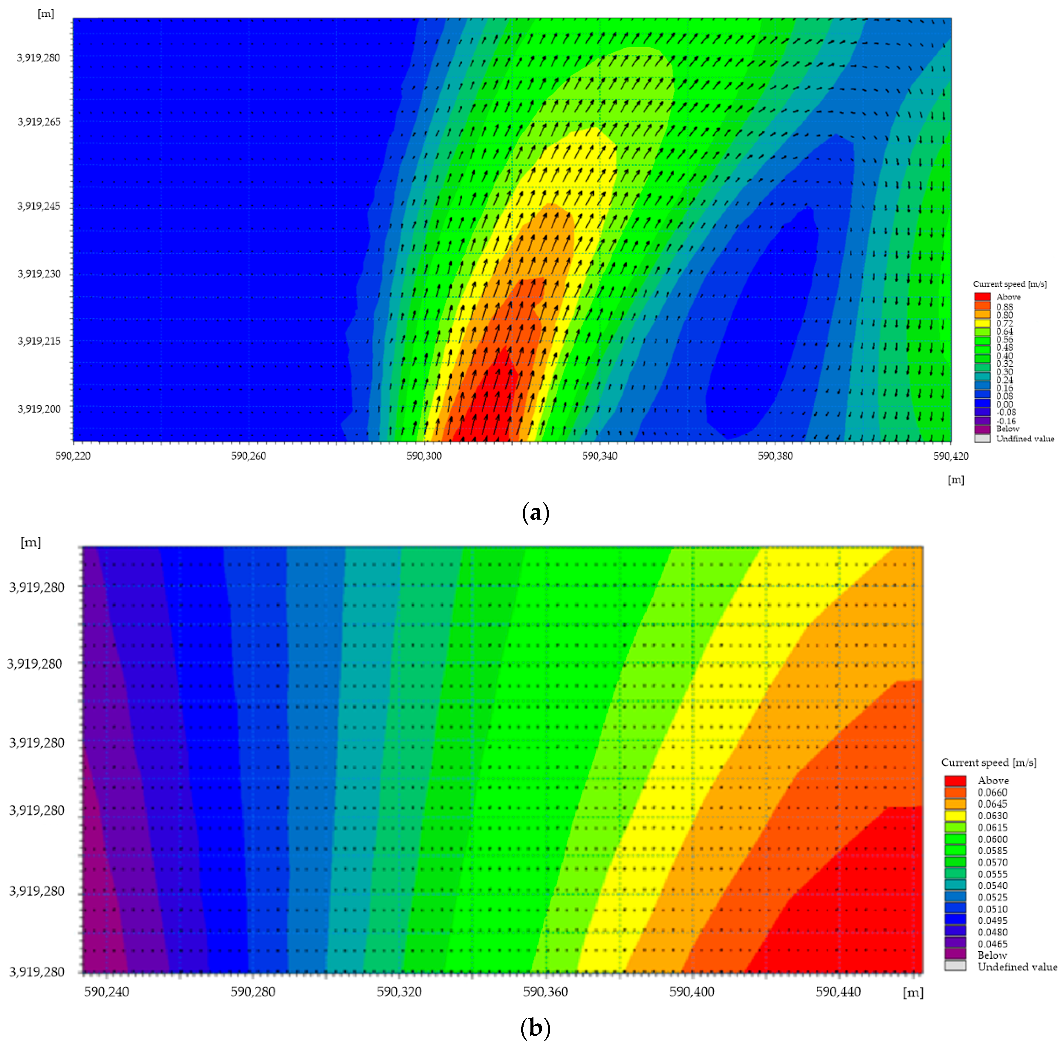
2.3.2. Analysis of Flow Velocity Field and Sediment

The entire water body of channel #1 in the sedimentation basin exhibits a small flow rate and a stable flow pattern. The main flow is located on the right side of the sedimentation basin with a maximum flow rate of 1.8 m/s. The flow velocity in the left area was clearly lower than that in the right area, the water exchange was weak, the static water disturbance was minor, the large area was in a stagnant water state, and the sedimentation basin only played the role of water storage.
Figure 7 shows the vectorial distribution of flow fields at the entrance, middle, and outlet of channel #1 of the sedimentation basin at a certain time. From the figure, it can be observed that (a) is the entrance, the coordinate range is (590,220, 3,919,190)~(590,420, 3,919,280), and there is a visible backflow; (b) is the middle reaches, the coordinate range is (590,230, 3,920,270)~(590,460, 3,920,380), the flow rate of upstream water in the channel is low, and the maximum flow rate does not exceed 0.1 m/s; and (c) is the exit, the coordinate range is (590,260, 3,921,380)~(590,520, 3,921,500), the flow rate gradually increases, and the maximum flow rate is approximately 0.75 m/s. There is visible reflux because the flow velocity in the upstream and middle reaches is higher than that in the entire area of the sedimentation basin, and there are differences in size and direction to form the reflux pattern. In Figure 7c, the flow rate increases gradually owing to the sudden decrease in the cross-section. The color represents the velocity, and the arrow represents the size and direction of the velocity.
Because of the large flow velocity at the entrance of the sedimentation basin, the flow velocity and sediment-carrying capacity gradually decrease during the course, and there is not enough power to make the sediment continue to move downstream. Thus, the overall sediment of the channel mainly falls and silts in the middle and upper reaches and is concentrated in the longitudinal coordinates at approximately 39,193.3 km and 391.2 km. Figure 8 shows the local silting distribution of channel #1 in the sedimentation basin in 2019. Figure 8 shows that sediment deposits are evident on the right side of the channel; (a) vertical coordinate is near 3,919,300 m, and the coordinate range is (590,395, 3,919,320)~(590,425, 3,919,338); and (b) vertical coordinate is near 3,912,000 m, and the coordinate range is (590,150, 3,919,900)~(590,450, 3,920,040). The legend represents silting thickness. The maximum deposit thickness near the longitudinal coordinate of 3,912,000 m is approximately 3.5 m, and the degree of siltation on the left side is relatively small and is related to the flow field distribution on the left side.
In this research, the horizontal and vertical coordinates in the channel #1 topography of the sedimentation basin were used as the X and Y coordinates, and the sediment thickness in the sedimentation basin was used as the Z coordinate. The data interpolation method in the Surfer geographic information software was used to calculate the sediment volume. According to calculations, the annual silting volume of channel #1 in the sedimentation basin was approximately 3.32 million m3, and the volume of the sedimentation basin was approximately 4.05 million m3 in 2019. The silting volume of the sedimentation basin was close to the designed storage capacity of the sedimentation basin, and the service life of a single channel was less than one year. The ability to achieve sediment settling was weakened, which affected the regular use of sedimentation basins. Therefore, it is necessary to optimize the operation scheme of the sedimentation basin and improve its service effects.

3. Optimization Analysis of Operation Scheme

According to the measured data of the sedimentation basin, the maximum sand content at the outlet from 16 August 2020 to 13 December 2020 was approximately 1.95 kg/m³. The minimum sediment concentration was approximately 0.036 kg/m3, and the average sediment concentration was approximately 0.34 kg/m3. Regulations on irrigation management of the Lower Yellow River diversion indicate that the irrigation channel “sediment content of backwater shall not exceed 2 kg/m3”, the sediment content of the outlet meets the requirements, and the average sediment content is much lower than 2 kg/m3. At the same time, a large part of the reservoir capacity has not been utilized, and the left part of the channel only plays the role of water storage in the actual measured silting situation of the sedimentation basin. In the future, water diversion processes should be considered to increase sediment concentration at the outlet, reduce sediment deposition in the sedimentation basin, and improve the sediment settling effect subject to the condition of ensuring water diversion safety.
In addition, during the operation of the sedimentation basin affected by incoming water and sediment in flood and non-flood seasons, water diversion indexes in different periods are determined according to the actual conditions in the flood and non-flood sea-sons.

3.1. Setting of Boundary Conditions

3.1.1. Basis for Boundary Setting

The water intake of the diversion project from the Yellow River Diversion Project was located downstream of the Xiaolangdi Reservoir and was regulated by it. Figure 9 shows the flow changes of the Xiaolangdi Reservoir in 2012, 2018, and 2019, which show that the flow of the Xiaolangdi Reservoir is not uniform in time distribution, and the flow changes are apparent in flood and non-flood seasons. According to the measured data, the average daily flow in the flood season was approximately twice that in the non-flood season.
According to the fitting curve of the flow–sediment content of Shi et al. [31] and Wang et al. [32], the flow rate was determined to be proportional to the sediment content. Based on the actual measured sediment concentration, silt status, and analysis of incoming water and sediment in additional periods, this study adopted measures to change the operating level of the outlet in different diversion and sediment diversion conditions to artificially regulate the distribution of sediment deposition and improve the sediment settlement effect of the sedimentation basin.
In this research, the year was divided into flood and non-flood seasons. The mathematical model was established using channel #1 of the sedimentation basin, different schemes were set according to water and sediment conditions, and simulation calculations were conducted. According to the simulation results, the sediment deposition laws in each scheme were analyzed, and the operation mode of the sedimentation basin was optimized scientifically and reasonably.

3.1.2. Model Boundary Condition Setting

According to the actual measurement of the sedimentation basin from 2017 to 2020 and the analysis of flow change of the Xiaolangdi Reservoir, the index setting of flow and sediment concentrations in the flood and non-flood seasons was determined.
By adjusting the operating water level at the outlet of the sedimentation basin, in this study, the distribution of sediment deposition was regulated at different diversion and sediment diversion conditions to improve the settling effect of the sedimentation basin. Using channel #1 of the sedimentation basin as an object, the water and sediment models in the flood and non-flood seasons were established by adopting measures to change the functional level of the outlet.

3.2. Scheme Setup

Using Mike 21 software, taking channel #1 of the sedimentation basin as the research object, the flood and sediment models in the flood season and non-flood seasons were established.
Scheme I: Setting the upper-boundary condition of the hydrodynamic module, the flood season is the flow process in Figure 10, and the non-flood season is the flow process in Figure 10. The lower-boundary conditions are raised by 0.5 m in the raw water level data. The upper-boundary condition of the sediment module is set up. The flood season is the sediment concentration process in Figure 10, the non-flood season is the sediment concentration process in Figure 11, and the lower-boundary condition has a zero gradient.
In scheme II, the upper-boundary condition of the hydrodynamic module is set. The flow in the flood season is the flow process shown in Figure 10, the flow process in the non-flood season is shown in Figure 11, and the lower-boundary conditions are the raw water level data. The upper-boundary condition of the sediment module is set up. The flood season is the sediment concentration process in Figure 10, the non-flood season is the sediment concentration process in Figure 11, and the lower-boundary condition has a zero gradient.
Scheme III: In the setup of the upper-boundary condition of the hydrodynamic module, the flood season is the flow process shown in Figure 10, and the non-flood season is the flow process shown in Figure 11. The lower-boundary conditions are reduced by 0.5 m in the raw water level data. The upper-boundary condition of the sediment module is set up. The flood season is the sediment concentration process in Figure 10, the non-flood season is the sediment concentration process in Figure 11, and the lower-boundary condition has a zero gradient.
In the same model, except for the lower-boundary water level, the other conditions are consistent in the same year. In the same period, the simulation results of schemes I, II, and III are compared with each other, and the simulation results of the same scheme in the flood and non-flood seasons are compared with each other. The effects of sediment settling of the sedimentation basin are respectively analyzed with single and dual channels as research objects.

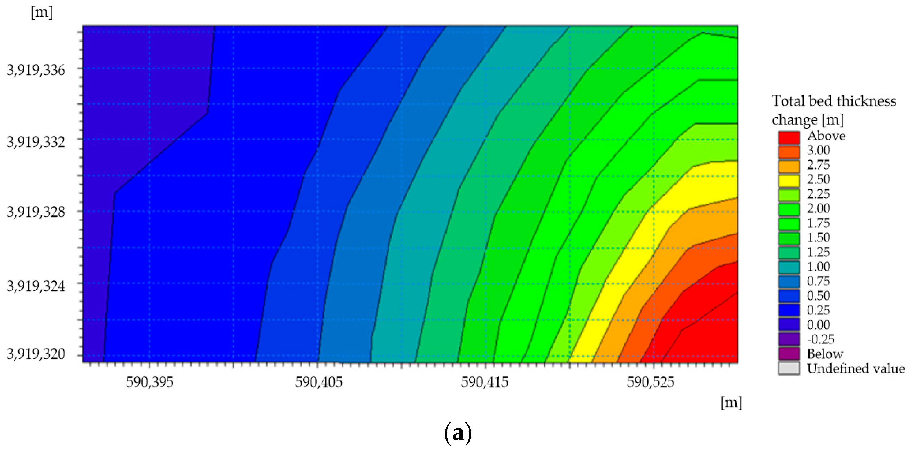
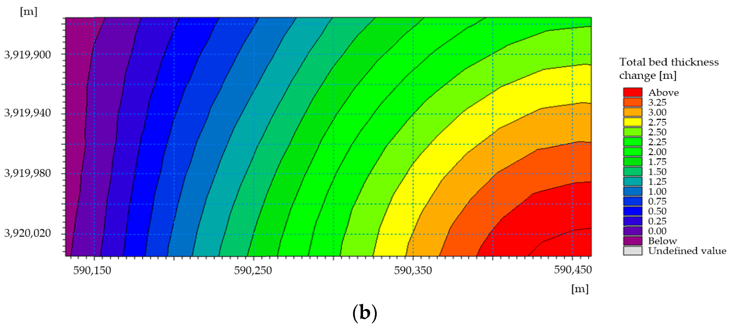
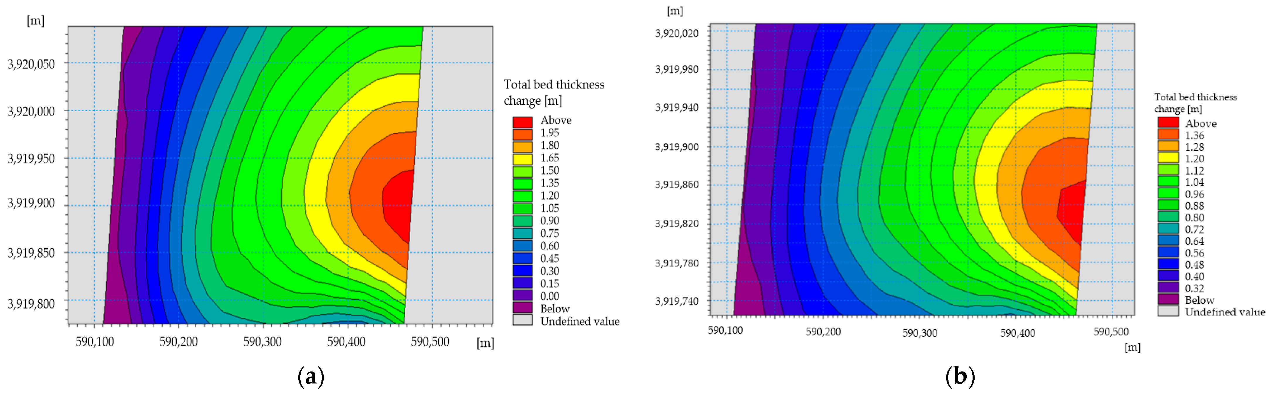
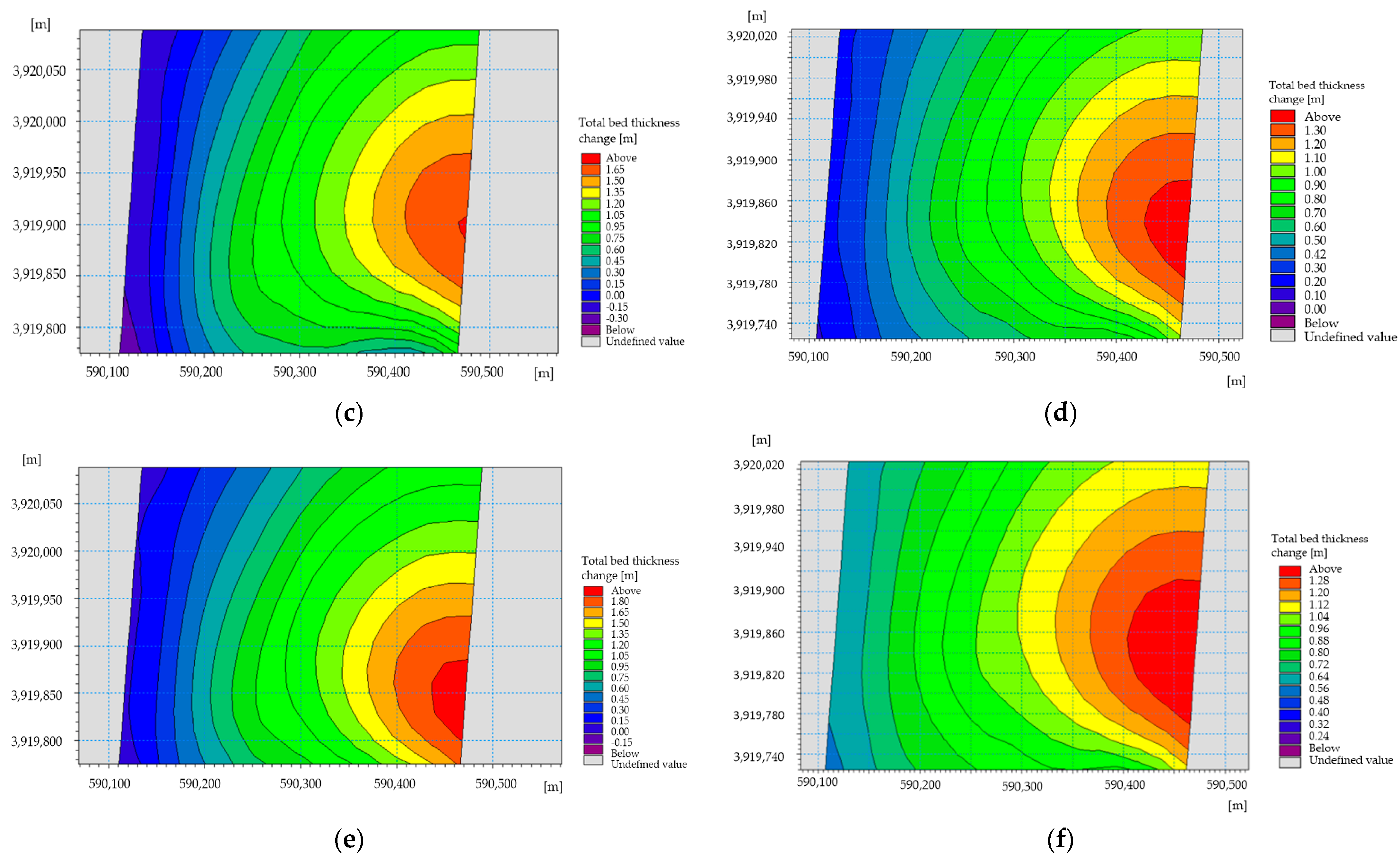
3.3. Results and Discussion

The variation rule of sediment concentration at the four characteristic points shown in Figure 5 was analyzed. As shown in Figure 12, (a) is scheme I flood season, (b) is scheme I non-flood season, (c) is scheme II flood season, (d) is scheme II non-flood season, (e) is scheme III flood season, and (f) is scheme III non-flood season. During the flood season, the maximum sediment concentration at the distinct points of outlet water level elevation and lowering were close to the maximum sediment concentration of the original water level. In the non-flood season, the influence of the elevation or lowering of the outlet water level on the outlet sediment concentration was not apparent. It can be observed from the variation rule of characteristic points T1–T4 that the sediment content closer to the outlet was lower, that is, the sediment content at T1 was lower than that at T4. Among the three schemes, the sediment concentration of diversion in the flood season was approximately twice that of the non-flood season, and the sediment concentration at the outlet was higher than that in the non-flood season.
Figure 13 shows local silting distributions for different schemes: (a) is scheme I flood season, with the coordinate range of (590,100, 3,919,800)~(590,500, 3,919,850); (b) is scheme I non-flood season, with the coordinate range of (590,100, 3,919,740)~(590,500, 3,920,020); (c) is scheme II flood season, with the coordinate range of (590,100, 3,919,800)~(590,500, 3,920,050); (d) is scheme II non-flood season, with the coordinate range of (590,100, 3,919,740)~(590,600, 3,920,020); (e) is scheme III flood season, with the coordinate range of (590,100, 3,919,800)~(590,500, 3,920,050); (f) is scheme III non-flood season, with the coordinate range of (590,100, 3,919,740)~(590,500, 3,920,020); and color legends represent the silting thickness. Figure 13 shows that in the flood season, the maximum silting thickness of the three schemes was reached at a longitudinal coordinate of approximately 3,919,900 m, and the maximum silting consistency of the elevated water level was approximately 2.1 m, which is higher than those of the other two schemes. In the non-flood season, the maximum silting thickness of the three schemes was reached at a longitudinal coordinate of approximately 3,919,840 m, and the maximum silting consistency of the lowered water level was approximately 1.36 m, which is lower than those of the other two schemes.
From the silting thickness contour diagram of the three schemes, it can be observed that the distribution of the silting area with a reduced water level is more uniform. The left-most silting thicknesses of the channel in the flood and non-flood seasons are approximately 0.2 and 0.64 m, respectively. The distribution of the silting area in the non-flood season is more prominent, the silting condition of the silting basin is improved, and the utilization ratio of the channel is higher. Among the three schemes, the sediment concentration of diversion in the flood season and the maximum silting thickness are approximately 1.5 times those in the non-flood season.
Table 1 shows the sediment deposition in the different schemes. When the outlet water level decreased, sediment deposition decreased. During the flood and non-flood season, the amount of sedimentation at low water levels (scheme III) was reduced by 180,000 and 150,000 m3, respectively, compared with the high water level (scheme I).
It can be concluded that the outlet water level was reduced, the ratio drop of water depth increased, the flow velocity and sediment-carrying capacity increased, the sediment was transported downstream of the channel along the river, and the sediment concentration at the outlet increased slightly but still met the design requirements. The total sediment deposition in the channel was reduced. In conclusion, the silting volume of the outlet low-water-level operation (scheme III) was significantly lower than those of the first two schemes, which can increase the service life of the sedimentation basin and prolong the period of silting removal by about 3.5 months.

4. Conclusions

This research used the sedimentation basin of the Yellow River Diversion Project as the research object, based on the Mike 21 model, to discuss the simulation of an optimization scheme, and compared the three schemes of a raised outlet water level, original water level, and a lowered outlet water level. Through the automatic control technology of water level, the outlet water level can be adjusted by using the outlet sluice. The optimal scheme was determined as scheme III; the water level at the outlet was lowered by 0.5 m. The results show that during the flood and non-flood seasons, the amount of sedimentation during the high-water outlet operation (scheme I) increased by 180,000 m3 and 150,000 m3, respectively, compared with the low-water outlet operation (scheme III). Combined with the distribution of sediment deposition, it is concluded that when the outlet water level is lowered, the distribution of sediment deposition in the sedimentation basin is more uniform, the sedimentation condition in the sedimentation basin is also improved, the utilization ratio of the channel is higher, and the period of silting removal is prolonged by about 3.5 months. This research provides a scientific and feasible idea for efficient utilization of the sedimentation basin, and the results are easy to observe and compare. However, it only considered the channel sedimentation basin and did not consider the swirling type, inclined-plate type, circular middle-ring, and other sedimentation basins of hydraulic engineering; therefore further research is needed.

Author Contributions

Conceptualization, J.Y.; methodology, M.C.; formal analysis, M.C.; data curation, M.C. and Q.L.; writing—original draft, M.C. and Q.L.; writing—review and editing, J.Y. and L.X.; supervision, H.S. and N.H. All authors have read and agreed to the published version of the manuscript.

Funding

This research was funded by the Special Project of the National Natural Science Fund (grant number 42041006), Key Project of the National Natural Science Fund (Grant No. HKY-JBYW-2018-03, HKY-JBYW-2020-15), Open Research Fund of the State Key Laboratory of Simulation and Regulation of Water Cycle in River Basin (Grant No. IWHR-SKL-KF202004), and Hubei Key Laboratory of Disaster Prevention and Mitigation (China Three Gorges University) (Grant No. 2021KJZ04).

Informed Consent Statement

Informed consent was obtained from all subjects involved in the study.

Data Availability Statement

The data presented in this study are available on request from the corresponding author.

Acknowledgments

We would like to thank the reviewer for their valuable comments and suggestions, to the editors for their serious and responsible attitude, to the publisher for this valuable opportunity. We also thank our other colleagues’ valuable comments and suggestions that helped improve the manuscript.

Conflicts of Interest

The authors declare no conflict of interest.

References

  1. Ministry of Water Resources of the People’s Republic of China. Design Specification for Sedimentation Basin of Water Conservancy and Hydropower Project: SL 269-2001[S]; China Water Resources and Hydropower Press: Beijing, China, 2001; pp. 22–34. [Google Scholar]
  2. Bagnold, R.A. Bed load transport by natural rivers. Water Resour. Res. 1977, 13, 303–312. [Google Scholar] [CrossRef]
  3. Zee, C.H.; Zee, R. Formulas for the Transportation of Bed Load. J. Hydraul. Eng. 2017, 143, 04016101. [Google Scholar] [CrossRef]
  4. Chen, G.S.; Wang, Y.M.; Bai, T.; Du, H.H. Diagnoses of runoff-sediment relationship based on variable diagnostic method-variable step length sliding correlation coefficient method in Ning-Meng reach. Int. J. Hydrogen Energy 2016, 41, 15909–15918. [Google Scholar] [CrossRef]
  5. An, C.; Lu, J.; Qian, Y.; Wu, M.; Xiong, D. The scour-deposition characteristics of sediment fractions in desert aggrading rivers—Taking the upper reaches of the Yellow River as an example. Quat. Int. 2019, 523, 54–66. [Google Scholar] [CrossRef]
  6. Krishnappan, B.G.; Lau, Y.L. Turbulence Modeling of Flood Plain Flows. J. Hydraul. Eng. 1986, 112, 251–266. [Google Scholar] [CrossRef]
  7. Asgharzadeh, H.; Firoozabadi, B.; Afshin, H. Experimental investigation of effects of baffle configurations on the performance of a secondary sedimentation tank. Sci. Iran. 2011, 18, 938–949. [Google Scholar] [CrossRef] [Green Version]
  8. Bürger, R.; Careaga, J.; Diehl, S. A simulation model for settling tanks with varying cross-sectional area. Chem. Eng. Commun. 2017, 204, 1270–1281. [Google Scholar] [CrossRef]
  9. Wang, B.J.; Fu, X.D. Inter-annual variation characteristics of the relationship between sediment concentration and discharge in Huangfuchuan watershed. J. Appl. Fundam. Eng. Sci. 2020, 28, 642–651. [Google Scholar] [CrossRef]
  10. Saady, N.M.C. Utilizing settling tests to design a conventional upflow settling tank modified with inclined plates. Water Sci. Technol. 2012, 66, 858–864. [Google Scholar] [CrossRef] [PubMed]
  11. Shahrokhi, M.; Rostami, F.; Said, M.A.M. Numerical modeling of baffle location effects on the flow pattern of primary sedimentation tanks. Appl. Math. Model. 2013, 37, 4486–4496. [Google Scholar] [CrossRef]
  12. Kim, K.Y.; Park, S.; Lee, W.H.; Kim, J.O. Simulating the behavior of ballasted flocs in circular lamellar settling tank using computational fluid dynamics (CFD). Desalination Water Treat. 2020, 183, 23–29. [Google Scholar] [CrossRef]
  13. Tarpagkou, R.; Pantokratoras, A. CFD methodology for sedimentation tanks: The effect of secondary phase on fluid phase using DPM coupled calculations. Appl. Math. Model. 2013, 37, 3478–3494. [Google Scholar] [CrossRef]
  14. Liu, X.; Xue, H.; Hua, Z.; Yao, Q.; Hu, J. Inverse Calculation Model for Optimal Design of Rectangular Sedimentation Tanks. J. Environ. Eng. 2013, 139, 455–459. [Google Scholar] [CrossRef]
  15. Razmi, A.; Bakhtyar, R.; Firoozabadi, B.; Barry, D. Experiments and numerical modeling of baffle configuration effects on the performance of sedimentation tanks. Can. J. Civ. Eng. 2013, 40, 140–150. [Google Scholar] [CrossRef] [Green Version]
  16. Tarpagkou, R.; Pantokratoras, A. The influence of lamellar settler in sedimentation tanks for potable water treatment—A computational fluid dynamic study. Powder Technol. 2014, 268, 139–149. [Google Scholar] [CrossRef]
  17. Al-Sammarraee, M.; Chan, A.; Salim, S.M.; Mahabaleswar, U.S. Large-eddy simulations of particle sedimentation in a longitudinal sedimentation basin of a water treatment plant. Part I: Particle settling performance. Chem. Eng. J. 2009, 152, 307–314. [Google Scholar] [CrossRef]
  18. Liu, Y.L.; Zhang, P.; Wei, W. 2D Simulation of Effects of Position of Baffles on the Removal Rate of Solids in a Sedimentation Tank. Appl. Mech. Mater. 2012, 253–255, 861–864. [Google Scholar] [CrossRef]
  19. Liu, Y.; Zhang, P.; Wei, W. Simulation of effect of a baffle on the flow patterns and hydraulic efficiency in a sedimentation tank. Desalination Water Treat. 2016, 57, 25950–25959. [Google Scholar] [CrossRef]
  20. Olsen, N.R.; Kjellesvig, H.M. Three-dimensional numerical modelling of bed changes in a sand trap. J. Hydraul. Res. 1999, 37, 189–198. [Google Scholar] [CrossRef]
  21. Jayanti, S.; Narayanan, S. Computational Study of Particle-Eddy Interaction in Sedimentation Tanks. J. Environ. Eng. 2004, 130, 37–49. [Google Scholar] [CrossRef]
  22. Bajcar, T.; Steinman, F.; Širok, B.; Prešeren, T. Sedimentation efficiency of two continuously operating circular settling tanks with different inlet- and outlet arrangements. Chem. Eng. J. 2011, 178, 217–224. [Google Scholar] [CrossRef]
  23. Bajcar, T.; Gosar, L.; Širok, B.; Steinman, F.; Rak, G. Influence of flow field on sedimentation efficiency in a circular settling tank with peripheral inflow and central effluent. Chem. Eng. Process. Process Intensif. 2010, 49, 514–522. [Google Scholar] [CrossRef]
  24. Stamou, A.I.; Adams, E.W.; Rodi, W. Numerical modeling of flow and settling in primary rectangular clarifiers. J. Hydraul. Res. 1989, 27, 665–682. [Google Scholar] [CrossRef]
  25. Ramin, E.; Wágner, D.S.; Yde, L.; Binning, P.J.; Rasmussen, M.R.; Mikkelsen, P.S.; Plósz, B.G. A new settling velocity model to describe secondary sedimentation. Water Res. 2014, 66, 447–458. [Google Scholar] [CrossRef] [PubMed]
  26. Tamayol, A.; Firoozabadi, B.; Ashjari, M.A. Hydrodynamics of Secondary Settling Tanks and Increasing Their Performance Using Baffles. J. Environ. Eng. 2010, 136, 32–39. [Google Scholar] [CrossRef]
  27. Saeedi, E.; Behnamtalab, E.; Neyshabouri, S.A.A.S. Numerical simulation of baffle effect on the performance of sedimentation basin. Water Environ. J. 2018, 34, 212–222. [Google Scholar] [CrossRef]
  28. Guo, H.; Ki, S.J.; Oh, S.; Kim, Y.M.; Wang, S.; Kim, J.H. Numerical simulation of separation process for enhancing fine particle removal in tertiary sedimentation tank mounting adjustable baffle. Chem. Eng. Sci. 2017, 158, 21–29. [Google Scholar] [CrossRef]
  29. Vahidifar, S.; Saffarian, M.R.; Hajidavalloo, E. Introducing the theory of successful settling in order to evaluate and optimize the sedimentation tanks. Meccanica 2018, 53, 3477–3493. [Google Scholar] [CrossRef]
  30. Gupta, G. An experimental study of fabric development in plane-bed phases. Sediment. Geol. 1987, 53, 101–122. [Google Scholar] [CrossRef]
  31. Shi, W.; Wang, G.Q.; Shao, X.J. Influence of Floods from Different Source Areas on the Relationship between Discharge and Sediment Concentration in the Lower Yellow River. Prog. Water Sci. 2003, 14, 147–151. [Google Scholar] [CrossRef]
  32. Wang, K.; Li, Y.; Ren, S.; Yang, P. Prototype Observation of Flow Characteristics in an Inclined-Tube Settling Tank for Fine Sandy Water Treatment. Appl. Sci. 2020, 10, 3586. [Google Scholar] [CrossRef]
Figure 1. Geographic location of the Yellow River Diversion Gate in Qucun.
Coatings 12 00478 g001
Figure 2. Arrangement of sedimentation basin.
Coatings 12 00478 g002
Figure 3. Schematic of grid partition of channel #1 in sedimentation basin.
Coatings 12 00478 g003
Figure 4. Verification of sediment concentration at the outlet.
Coatings 12 00478 g004
Figure 5. Marking location of characteristic points, the coordinate range is (590,210, 3,921,290)~(590,610, 3,921,560). T1, T2, T3, and T4 are the four characteristic points selected at the outlet of the sedimentation basin.
Coatings 12 00478 g005
Figure 6. Variation regularity of sediment concentration at characteristic points.
Coatings 12 00478 g006
Figure 7. Local flow field in channel #1 of sedimentation basin. The color represents the velocity, and the arrow represents the size and direction of the velocity. (a) is the entrance, the coordinate range is (590,220, 3,919,190)~(590,420, 3,919,280). The speed is negative, which represents that the backflow occurs in the sedimentation basin opposite to the set positive direction; (b) is the middle reaches, the coordinate range is (590,230, 3,920,270)~(590,460, 3,920,380); (c) is the exit, the coordinate range is (590,260, 3,921,380)~(590,520, 3,921,500).
Coatings 12 00478 g007aCoatings 12 00478 g007b
Figure 8. Distribution of local sediment in channel #1 in sedimentation basin. The legend represents silting thickness. (a) vertical coordinates is near 3,919,300 m, the coordinate range is (590,395, 3,919,320)~(590,425, 3,919,338). The total bed thickness is negative, which represents the scouring in the sedimentation basin; (b) vertical coordinates is near 3,912,000 m, the coordinate range is (590,150, 3,919,900)~(590,450, 3,920,040).
Coatings 12 00478 g008aCoatings 12 00478 g008b
Figure 9. Flow change process of Xiaolangdi Reservoir.
Coatings 12 00478 g009
Figure 10. Flow–sediment concentration and sediment concentration variation process in flood season.
Coatings 12 00478 g010
Figure 11. Flow and sediment concentration changes in non-flood season.
Coatings 12 00478 g011
Figure 12. Variation of sediment concentration at characteristic points in flood season and non-flood season in different schemes, (a) is scheme I flood season, (b) is scheme I non-flood season, (c) is scheme II flood season, (d) is scheme II non-flood season, (e) is scheme III flood season, (f) is scheme III non-flood season.
Coatings 12 00478 g012aCoatings 12 00478 g012b
Figure 13. Distribution of local silting in flood and non-flood seasons, (a) is scheme I flood season, the coordinate range is (590,100, 3,919,800)~(590,500, 3,919,850), (b) is scheme I non-flood season, the coordinate range is (590,100, 3,919,740)~(590,500, 3,920,020), (c) is scheme II flood season, the coordinate range is (590,100, 3,919,800)~(590,500, 3,920,050), (d) is scheme II non-flood season, the coordinate range is (590,100, 3,919,740)~(590,600, 3,920,020), (e) is scheme III flood season, the coordinate range is (590,100, 3,919,800)~(590,500, 3,920,050), (f) is scheme III non-flood season, the coordinate range is (590,100, 3,919,740)~(590,500, 3,920,020). The total bed thickness is negative, which represents the scouring in the sedimentation basin.
Coatings 12 00478 g013aCoatings 12 00478 g013b
Table 1. Sediment deposition in different schemes.
Silting Volume (104 × m3)Scheme IScheme IIScheme III
Flood Season192186174
Non-Flood Season153149138
Publisher’s Note: MDPI stays neutral with regard to jurisdictional claims in published maps and institutional affiliations.

