Research on Dynamic Stress–Strain Change Rules of Rubber-Particle-Mixed Sand

Abstract

We conducted GDS dynamic triaxial tests to study the change rules of the hysteresis curve morphology, axial strain, dynamic elastic modulus, and damping ratio of waste tire rubber-mixed sand-based subgrade model samples with different rubber particle sizes, rubber mixing amounts, and loading times. The research revealed the developmental rule of the hysteresis curves of waste tire rubber-mixed-sand samples under cyclic loading. From the analyses and comparison of the dynamic stress–strain change rules of rubber-particle-mixed-sand samples under different test conditions, it was concluded that the dynamic elastic modulus and shear stiffness of rubber-mixed-sand samples were smaller than those of pure sand samples under cyclic loading while their damping ratios were greater than that of pure sand samples, promoting vibration resistance and reduction to a larger extent. Therefore, this conclusion is of guiding significance for engineering practice.

1. Introduction

Waste tire particles have damping characteristics because rubber has high elasticity and good stability. Rubber particles have a smaller elastic modulus than other modified reinforced materials, but they can recover from larger deformation and have greater elastic deformation ability when external forces are removed. In addition, there is no obvious yielding point on the stress–strain curves of rubber particles. All these indicate that rubber particles enjoy an excellent vibration reducing performance. At present, research on the static characteristics of waste tire particle-mixed soil dominates compared with that of dynamic characteristics in China and abroad. Some scholars have drawn valuable conclusions through tests.

Feng et al. [1] studied the dynamic stress–strain change rules of a mixture of sand and rubber particles via dynamic triaxial tests. The test results were then compared with the Hardinen conventional soil dynamic characteristics formula. As a result, an improved Hardinen formula of the dynamic characteristics of rubber-mixed sand was obtained.

Pamukcue et al. [2] studied the dynamic characteristics of a sand–rubber particle mixture through the resonant column test, from which it was concluded that a smaller stiffness of this mixture compared with pure sand results from the different dynamic modulus of the two materials and the increased contact area between particles. If there is a big difference in the expansion coefficients of the two materials, the damping ratio of mixed samples will be larger than that of pure sand.

Nakeh [3] studied the influences of dynamic stress and estimated the confining pressure on the dynamic elastic modulus of rubber-mixed sand in large-scale dynamic triaxial tests using the exponential function model.

Anasta et al. [4,5,6] studied the change rules of the dynamic elastic modulus and damping ratio of rubber-mixed sand under different test conditions in dynamic triaxial tests. The theoretical formulas for the dynamic elastic modulus and damping ratio of rubber-mixed sand were obtained through function fitting based on a large number of tests.

Sui X X [7] mixed quartz particles into sand and studied the dynamic elastic modulus and damping ratio of mixed sand samples under different test conditions via dynamic triaxial tests. It was concluded that the dynamic elastic modulus and damping ratio of mixed sand samples are proportional to the dynamic stress applied in the tests.

In dynamic triaxial tests, Li L H [8] found that the dynamic elastic modulus of waste tire particle-mixed sand is smaller than that of pure sand, and the equivalent damping significantly rises with the increase in rubber content.

Shang S P [9] studied the change rules of the dynamic elastic modulus of glass sand under different test conditions in dynamic triaxial tests. It was concluded that the dynamic shear modulus of rubber-glass-mixed sand decreases after rubber particles are added.

The application of discarded tires in geotechnical engineering, particularly soil reinforcement technology, has been extensively studied. The application of soil reinforcement technology dates back to antiquity. In ancient times, basic materials were combined with dirt to create rudimentary soil reinforcements. Recently, reinforcing technology has been implemented in geotechnical engineering, and reinforced materials have evolved from natural textiles and steel bars to geosynthetics such as geomembranes and geocells. Diverse soil-reinforcement materials are often lightweight, simple to assemble, inexpensive, and simple to produce and transport. In addition, reinforcing technology may raise soil strength, boost soil stability, and significantly enhance soil mechanical qualities [10,11,12,13].

To sum up, research on the dynamic characteristics of saturated sand dominates while that on the dynamic characteristics of waste tire rubber particles mixed with sand is inadequate. In this paper, GDS dynamic triaxial tests were conducted to study the change rules of the hysteresis curve, axial strain, dynamic elastic modulus, and damping ratio of waste tire rubber-mixed sand-based subgrade model samples with different rubber particle sizes, rubber mixing amounts, and loading times. Finally, conclusions of guiding significance for engineering practice were drawn from tests.

2. Test Content and Scheme

2.1. Test Instruments and Functions

2.1.1. Composition of Dynamic Triaxial Apparatus System DYNTTS

The dynamic triaxial apparatus system DYNTTS made in England was adopted in the tests, whose composition is shown in Figure 1. Specifically, the data acquisition system consisted of a distributed control system (DCS) signal receiver, an axial force sensor, and a pore water pressure sensor, and the external control system was composed of an axial force controller, a pressure chamber, a confining pressure controller, and a back pressure controller.

2.1.2. Experimental Principle of GDS Dynamic Triaxial Apparatus

The test principle of the GDS dynamic triaxial apparatus is that the confining pressure value ${\sigma }_3$ and the back pressure value P⁰ are preset via the confining pressure controller and the back pressure controller. Dynamic loads or static loads are applied to control force or displacement by operating GDSLAP when each set of confining pressure and back pressure reaches the test target values. GDSLAP coordinates and controls the relationship among the confining pressure controller, the back pressure controller, and the axial displacement force control system and processes the data collected by each sensor according to the set calculation mode. Then, the difference between the actual and target values is identified during the test before each set of data generated during the test is output. The details are as follows:

The initial diameter and height of the triaxial sample were set to be $D_0$ and $H_0$, respectively. The initial area $A_0$ and initial volume $V_0$ of the sample can be obtained according to Formulas (1) and (2).

$$V_0=\frac{\pi D_0^2{H}_0}{4}$$

(1)

$$A_0=\frac{\pi D_0^2}{4}$$

(2)

$D$, $H$, $A$, and $V$ represent the sample’s diameter, height, area, and volume, respectively. The volume change of the sample is obtained as $\Delta V=V_0-V$, the volume change data of the back pressure controller reflect the pore water pressure changes, and the derivation formulas are obtained as follows: the axial force of actual sample $\sigma =F/A+{\sigma }_3$, the effective stress ${\sigma }_3^{\prime }={\sigma }_3-{\mathrm{u}}_{\mathrm{w}}$ derived from pore water pressure, the effective axial stress ${\sigma }^{\prime }=\sigma -{\mathrm{u}}_{\mathrm{w}}$, the axial strain ${\epsilon }_{\mathrm{a}}=(\Delta \mathrm{H}/{\mathrm{H}}_0)\times 100\%$, the radial strain ${\epsilon }_{\mathrm{r}}=\left[\left(-D+D_0\right)/D_0\right]\times 100\%$, and the deviator stress ${\sigma }_1={\sigma }_3^{\prime }\times K_{\mathrm{c}}-{\sigma }_3^{\prime }$ derived from effective consolidation confining pressure ${\sigma }_3^{\prime }$ and consolidation ratio $K_{\mathrm{c}}$.

2.2. Test Scheme and Damage Standard

2.2.1. Test Scheme

A sinusoidal load with a stress amplitude of 30 kPa, a frequency of 1 Hz, and a vibration frequency of 300 times was applied via stress control in the dynamic pore pressure test of saturated rubber-mixed sand samples, and the parameters of dynamic stress, dynamic strain, and dynamic pore pressure were recorded in GDSLAP. The test was stopped when the dynamic pore pressure reached the damage standard, or the vibration frequency reached 300 s, the scheme of which is shown in

Table 1. Experimental scheme for research on dynamic pore pressure of rubber-mixed sand.

Mixing Amount/%	Particle Size/mm	Consolidation Stress Ratio	Confining Pressure/kPa	Dynamic Stress/kPa
10%	0.75	1	50, 100, 150	30
	1.5	1, 1.5, 2	50, 100, 150	30
	2.5	1	50, 100, 150	30
20%	0.75	1	50, 100, 150	30
	1.5	1, 1.5, 2	50, 100, 150	30
	2.5	1	50, 100, 150	30
30%	0.75	1	50, 100, 150	30
	1.5	1, 1.5, 2	50, 100, 150	30
	2.5	1	50, 100, 150	30

.

2.2.2. Damage Standard

Pore pressure standard was adopted in the research on dynamic pore pressure and hysteresis curve of samples; that is, the samples were damaged when the over-consolidation stress ratio ${\mathrm{u}}_{\mathrm{d}}/{\sigma }_3=1$. The pores in soil mass were compressed, and the dynamic pore water pressure between particles continuously increased under the cyclic action of dynamic loads. When the dynamic pore water pressure was equal to the effective confining pressure ($u_d={\sigma }_3$), the effective stress between particles of soil mass in the samples approached zero, leading to liquefaction damage of the soil mass.

2.3. Test Procedures

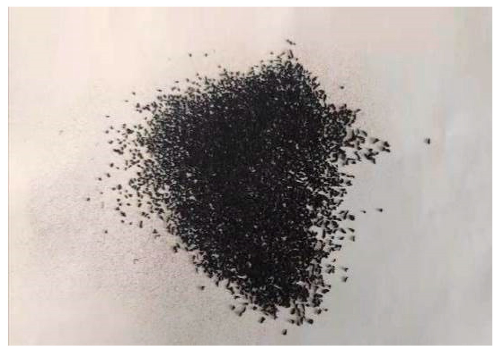
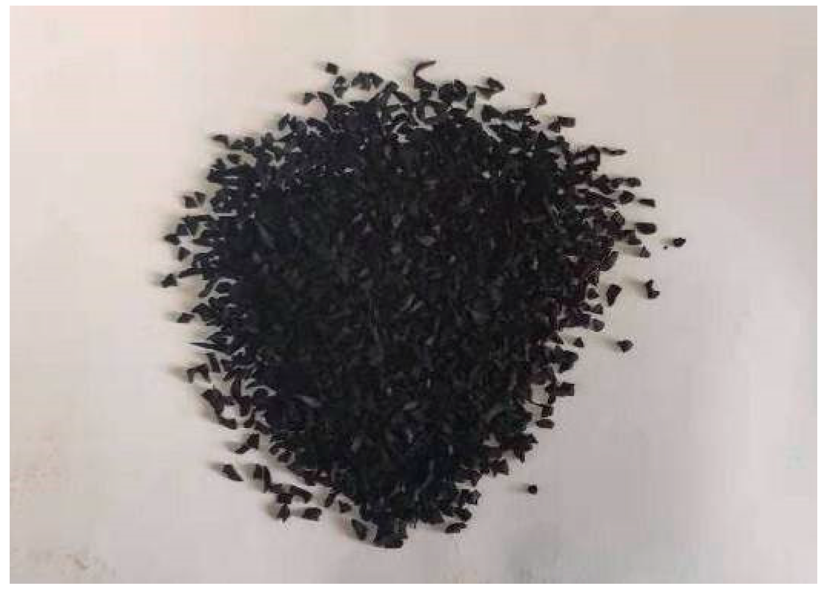
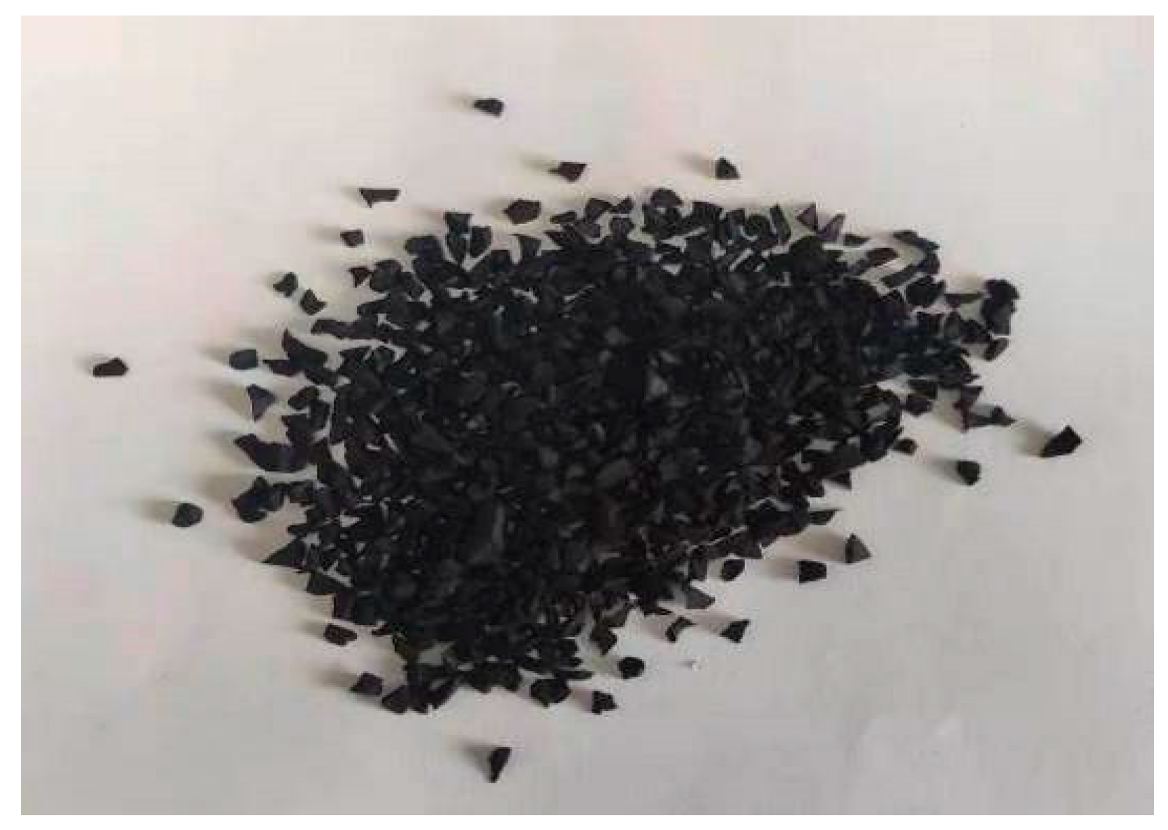
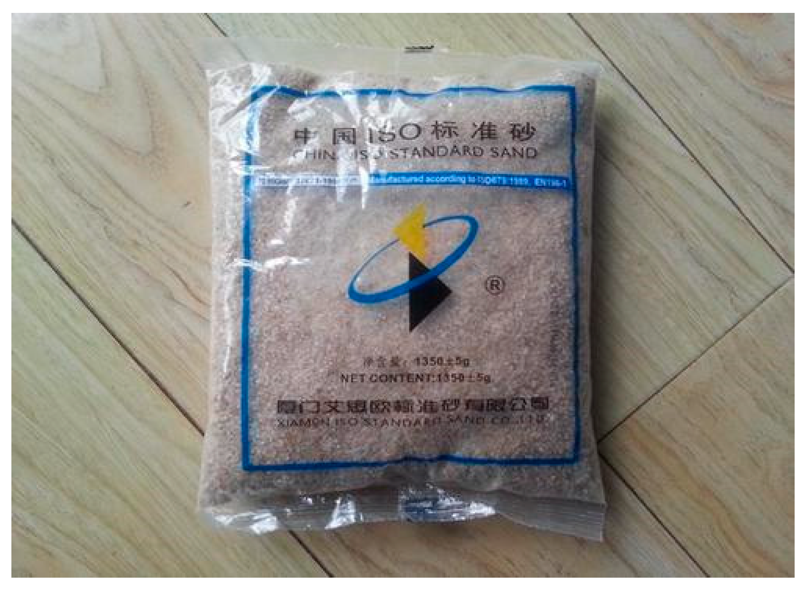
2.3.1. Test Materials and Sample Preparation

(1) Rubber particles. The rubber particles used in this test were produced via the normal temperature crushing method. Screened by the vibrating screen in the laboratory, the following three kinds of rubber particles with average particle sizes of 0.75 mm, 1.5 mm, and 2.5 mm, respectively, were mainly utilized, as shown in Figure 2, Figure 3, Figure 4 and Figure 5.

(2) Sand particles. ISO Fujian standard sand (as shown in Figure 5) was used as sand material in the tests to ensure the consistency of each group of tests. In addition, the density bottle method was adopted to measure the specific density (2.60) of sand in a dry state.

(3) Preparation of raw materials for dynamic triaxial test samples: waste tire rubber particles (three kinds of particle sizes) and Fujian standard sand. Tools for sample preparation: rubber membranes, three-segment dies, permeable stones, and filter paper.

To ensure the consistent arrangement of sand particles in each group of samples, the dry density of sand in rubber-mixed sand samples was required to be equal to that of pure sand samples when different contents of rubber particles were mixed into sand particles. The calculation formula for the corresponding proportion is shown as follows.

$$\rho =\frac{M_s}{V_s+V_k}=\frac{M_o-M_x}{V_o-V_x}$$

(3)

where $V_o$, $V_x$, $V_S$, and $V_k$ represent the total volume of rubber-mixed sand, the rubber volume, the sand volume, and the pore volume between particles, respectively, while $M_o$, $M_S$, and $M_x$ stand for the total mass of samples, the mass of sand particles, and the mass of rubber particles, respectively.

2.3.2. Installation, Saturation, and Consolidation of Samples

(1) Sample installation: The rubber-mixed sand was sampled via the moist sampling method, and the rubber-mixed sand particles were weighed according to the proportion which was boiled in water and cooled for 12 h for later use. The apparatus was normally plugged in, and all pipes were not blocked before the sample was installed. First, a permeable stone covered with moist single-layer filter paper was put on the base of the apparatus. Then, a three-segment die was installed, and the boiled and cooled rubber-mixed sand was put into the rubber membrane evenly and slowly. After the sand loading, the back pressure was set to be −30 kPa. When the back pressure loading was stable, the three-segment die was removed. At this moment, the sample was upright due to negative pressure, as shown in Figure 6. After that, the external pressure hood was closed, the apparatus was filled with water, and the axial force sensor value was set to 0.005 kN when the apparatus base rose and contacted the top sensor. When the axial force reached 0.005 kN, the apparatus no longer rose. The sample was contacted with the axial force sensor as shown in Figure 7. Then, the vent plug at the top of the pressure chamber was opened, and the inlet valve was opened to fill the pressure chamber with water. Finally, the inlet valve and the vent plug were closed after all steps were conducted.

(2) Sample saturation: Water head saturation and back pressure saturation were utilized to saturate the samples, thus improving the saturation of the rubber-mixed sand samples. First, water head saturation was performed. Specifically, the drain valve of the apparatus base was connected with that of the water container. Then, the drain valve of the container was opened so that the boiled and cooled distilled water flowed into the bottom from the apparatus base. In this way, the pores between sample particles were filled with water, and the air in the samples was exhausted, thus gradually elevating the saturation of the samples. In addition, excess distilled water flowed out from the top of the samples to the container prepared in advance. After the water head saturation, a small amount of air remained in the samples. However, the air in the samples was melted into water by applying five-level back pressure saturation. Figure 8 shows the five-level back pressure loading change curve. In the process of back pressure loading, the effective confining pressure remained at 20 kPa (the confining pressure remained greater than the back pressure to prevent the sample preparation from being damaged due to the overload of the dynamic pore pressure in the samples, and the five-level loading process could minimize the disturbance of the test apparatus loading on the samples). After the five-level back pressure loading, the saturation of the samples was detected. If the B value $\Delta u/\Delta {\sigma }_3>0.95$, the saturation condition was met. If not, saturation detection was conducted after the samples were re-installed and the saturation process was reloaded.

3. Research on Dynamic Stress–Strain Change Rules of Rubber-Particle-Mixed Sand

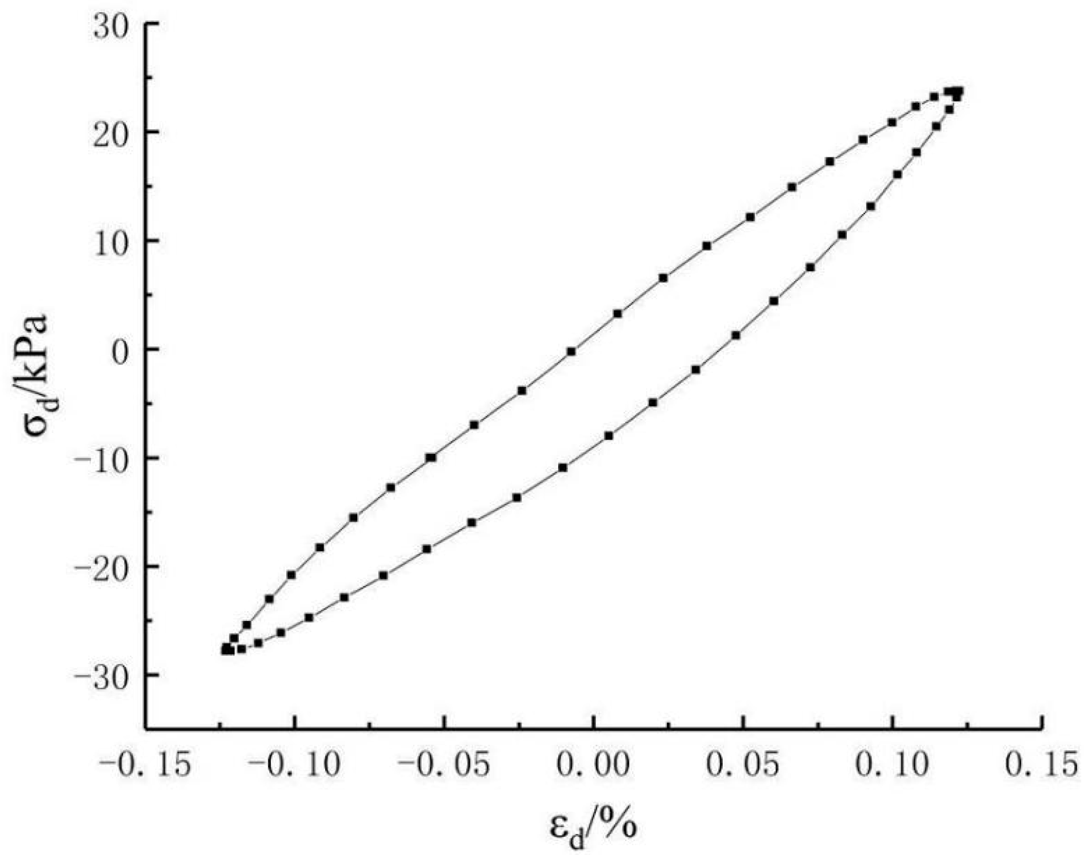
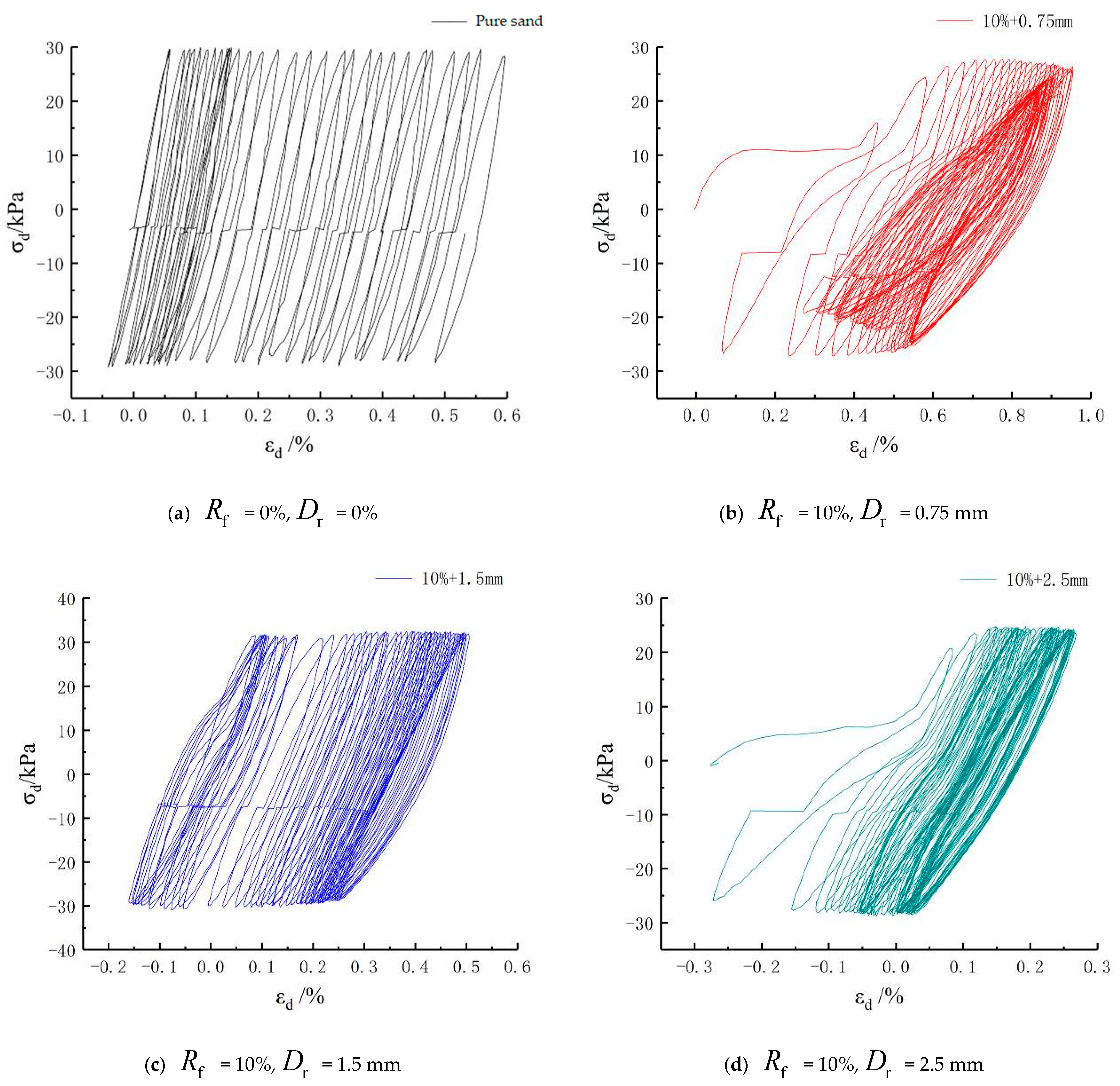
3.1. Change Rules of the Dynamic Stress–Strain Hysteresis Curve

The dynamic stress–strain relationship of the soil mass presents two characteristics under cyclic loading, namely nonlinearity and hysteresis. As shown in Figure 9, the stress–strain data points recorded in the dynamic triaxial tests were connected into a curve called a stress–strain hysteresis curve. The stress–strain hysteresis curve is a developmental curve where loading and unloading repeat cyclically, reflecting the relationship between the dynamic stress ${\sigma }_{\mathrm{d}}$ and the dynamic strain ${\epsilon }_{\mathrm{d}}$ at every moment during the cycle of the dynamic stress cyclic loading. The hysteresis of the dynamic stress–strain hysteresis curve was mainly displayed as the dynamic stress–strain hysteresis curve would gradually move towards the direction where strain magnified with the increase in cycle time since the soil mass was an elastoplastic material. The encircled central point shifted from the original point to the positive X-axis direction and the soil mass was subjected to unrecoverable permanent strain.

Research on Hysteresis Curve Morphology of Rubber-Particle-Mixed Sand

As the dynamic loading frequency in the test was 1 Hz and the interval of the data recording was set as 0.02 s, a total of 50 data points was acquired in the interval of 1 s. In order to analyze the change rules of the dynamic stress–strain hysteresis curve of the soil mass more meticulously, the hysteresis curves of the first 100 times of the cyclic loading recorded by the GDS operating system in the dynamic triaxial tests are exhibited in Figure 9.

Figure 10a–j is hysteresis curves of the soil samples in various groups with different mixing amounts of rubber particles. It was observed from the hysteresis curve of the pure sand in Figure 10a that cumulative strain took place in the pure sand samples under cyclic loading and the strain reached 0.54% after 100 times of vibration. The morphology of the hysteresis curves coincided at each time.

Figure 10b–d refers to the images of the hysteresis curves when the mixing amount of rubber $R_{\mathrm{f}}$ was 10%, and it was seen that the developmental rule of the hysteresis curves in three groups of samples all presented a trend from looseness to tightness. The samples showed a maximum strain of 0.95% within the range of vibration time while mixed with 0.75 mm rubber particles and the cumulative strain displayed an increasing trend. The strain range of the samples mixed with 1.5 mm rubber particles was −0.15%–0.47% and that of the samples mixed with 2.5 mm rubber particles was −0.25%–0.26%.

Figure 10e–g shows the images of the hysteresis curves with 20% mixing amount of rubber $R_{\mathrm{f}}$. The strain ranges of the samples mixed with rubber particles in the three sizes with the three mixing amounts were −0.41%–0.14%, −0.12%–0.27%, and −0.06%–0.13%, respectively. It was found that when the mixing amount of rubber increased to 20%, the range of the dynamic strain reduced correspondingly, and the central symmetry points of the hysteresis curves swung around the original points.

Figure 10h–j represents the images of the hysteresis curves with 30% mixing amount of rubber $R_{\mathrm{f}}$. The strain ranges of the samples mixed with rubber particles in the three sizes with the three mixing amounts were −0.28%–0.21%, −0.25%–0.06%, and −0.09%–0.23%, respectively. It was never discovered that a relatively large cumulative strain was produced in three groups of samples under cyclic loading. The morphology of the hysteresis curves was similar at each time and the central symmetry points of the hysteresis curves also swung around the original points.

The stress–strain hysteresis curve of the pure sand samples was taken as a reference object. As shown in Figure 1, with 100 times of vibration $N$, the strain ${\epsilon }_{\mathrm{d}}$ of the pure sand samples was 0.54% and the compressive strain of the samples increasingly enlarged until its damage as the test went on. Due to the high-resilience compressibility of rubber, the three groups of samples mixed with rubber particles in the size of 2.5 mm showed a different changing form in the stress–strain curve from the pure sand samples. In this case, the curve was presented as a reciprocating form of tension and compression and the strain fluctuated between −0.33% and 0.27%. It was figured out that the pure sand samples mixed with rubber particles acquired a greatly enhanced non-deformability. It was also observed that the strain change rates of the pure sand mixed with the rubber particles in the sizes of 1.5 mm and 0.75 mm were higher than that of the pure sand mixed with the rubber particles in the size of 2.5 mm. The strain of the samples mixed with the rubber particles in the size of 1.5 mm was between −0.26% and 0.42% and that of the samples mixed with the rubber particles in the size of 0.75 mm was between −0.36% and 0.95%. The rubber particles of a relatively large size could improve the non-deformability of the samples and the hysteresis curve of the samples mixed with such rubber particles presented a reciprocating form of tension and compression.

The influence of the mixing amount of rubber particles on the stress–strain relationship is expressed below. Under the cyclic loading, the compressive strain of the pure sand samples continuously increased until it was damaged. The stress–strain hysteresis curve of the rubber-mixed sand samples was similar to that of the pure sand samples because of a small mixing amount of rubber ($R_{\mathrm{f}}=10\%$). However, the samples with $R_{\mathrm{f}}=20\%$ and $R_{\mathrm{f}}=30\%$ had a stressed skeleton, in which the rubber particles were primary, on account of the large mixing amount of rubber particles, so the stress–strain hysteresis curve showed a totally different changing form from the pure sand. From the specific data in Figure 4, the strain range of the rubber particles in the three sizes was between −0.36% and 0.24% and the tensile and compressive strain was distributed. The strain of the samples with $R_{\mathrm{f}}=10\%$ changed from −0.19% to 0.9542% and the compressive strain dominated in the hysteresis curve, which was similar to that of the pure sand.

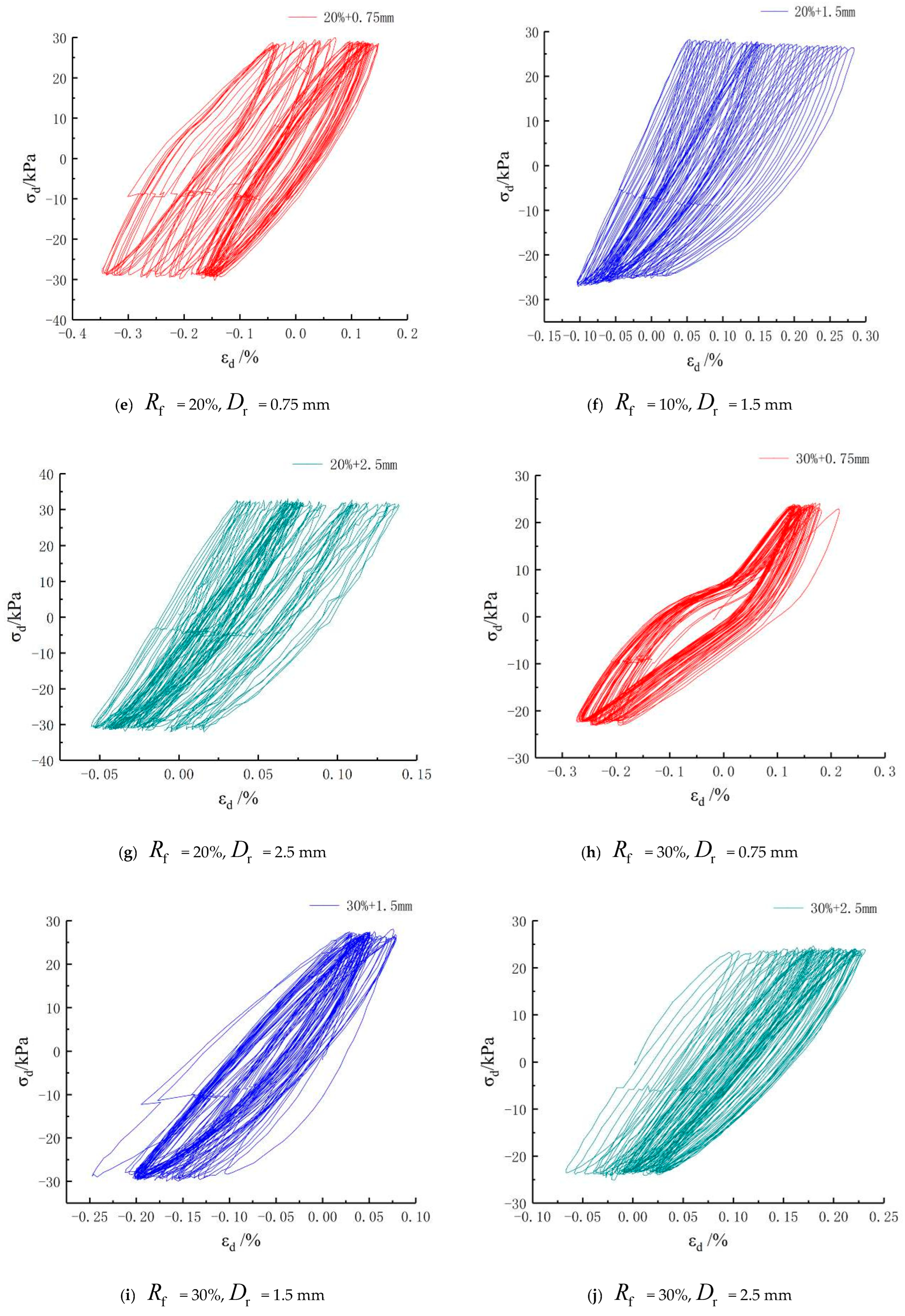
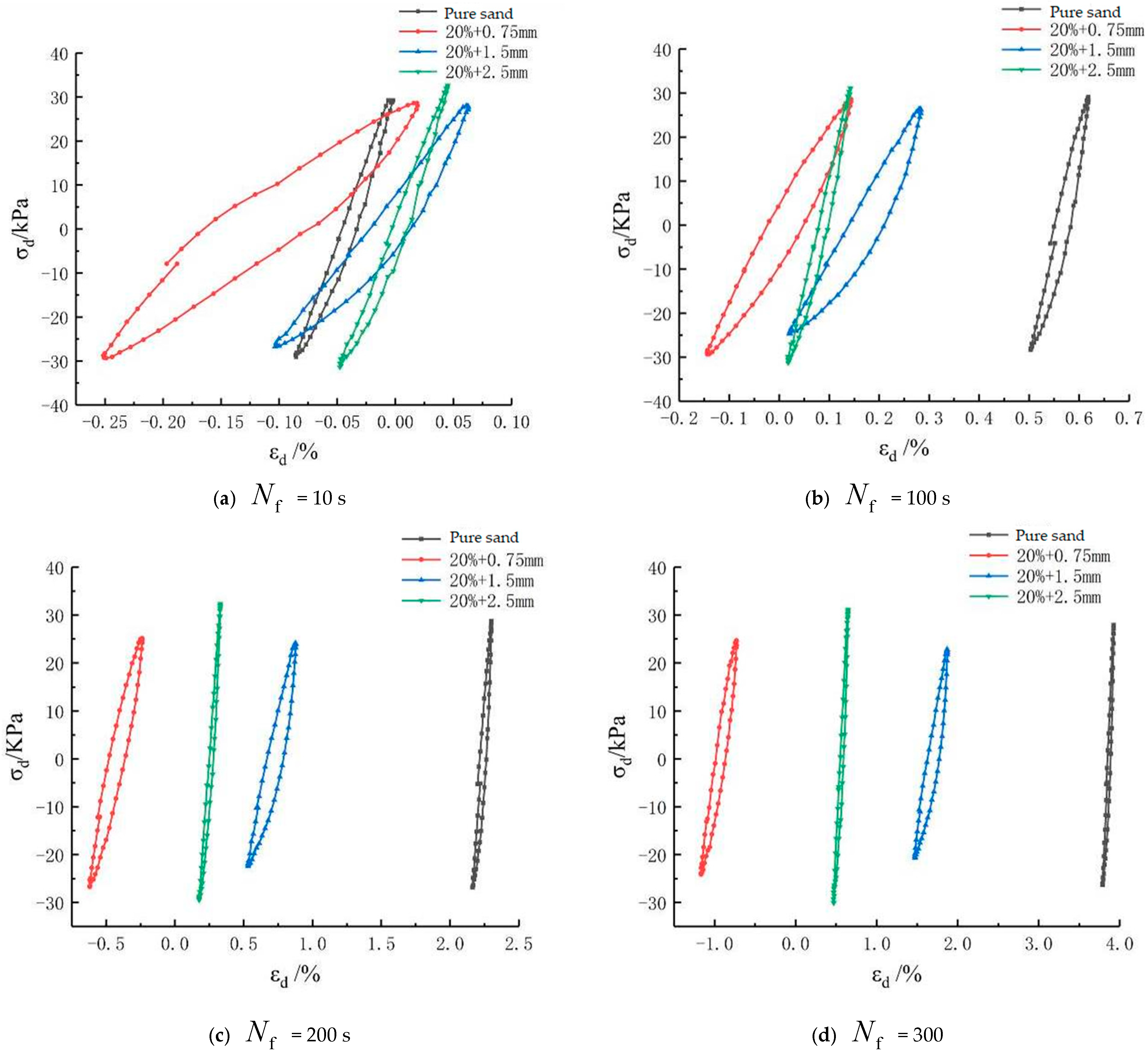
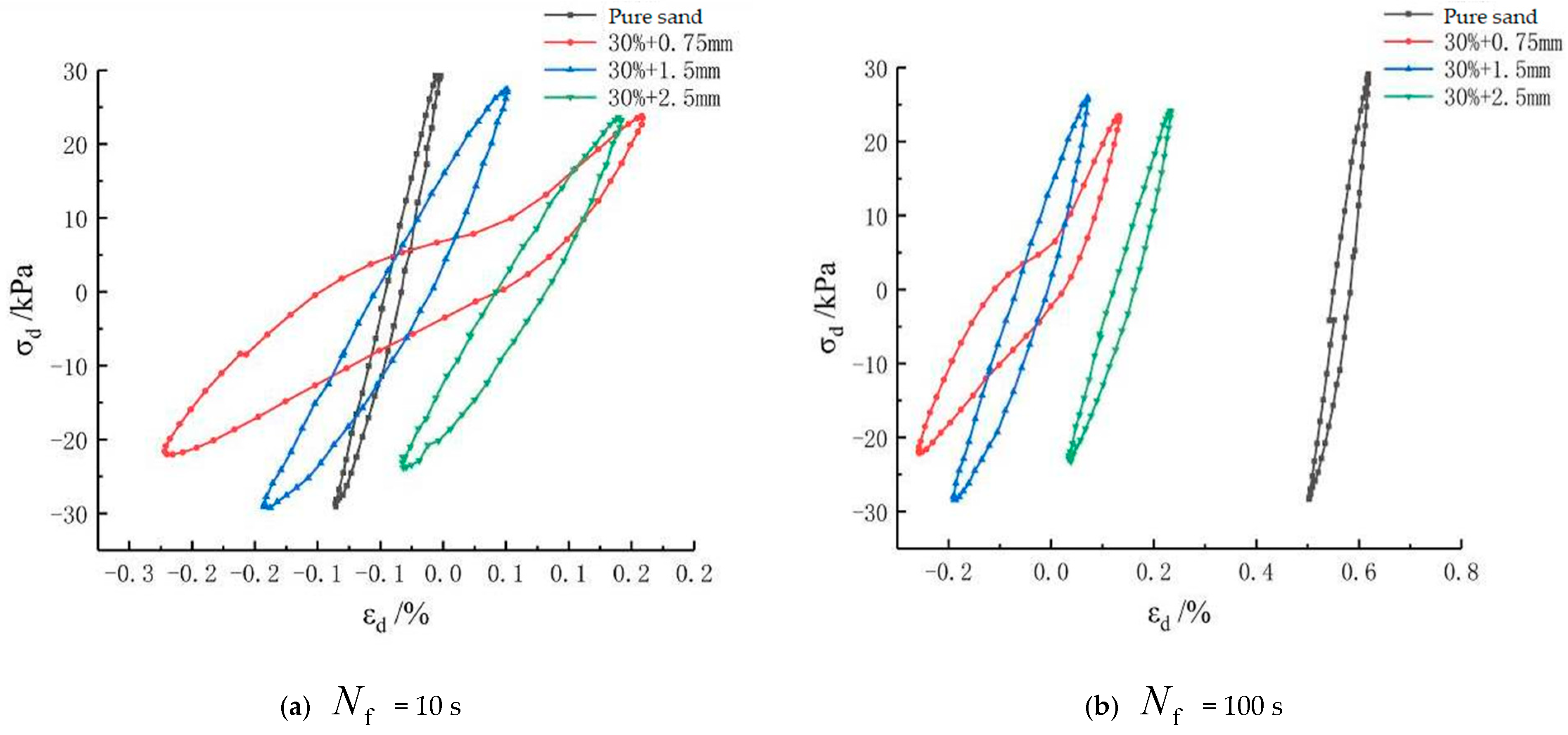
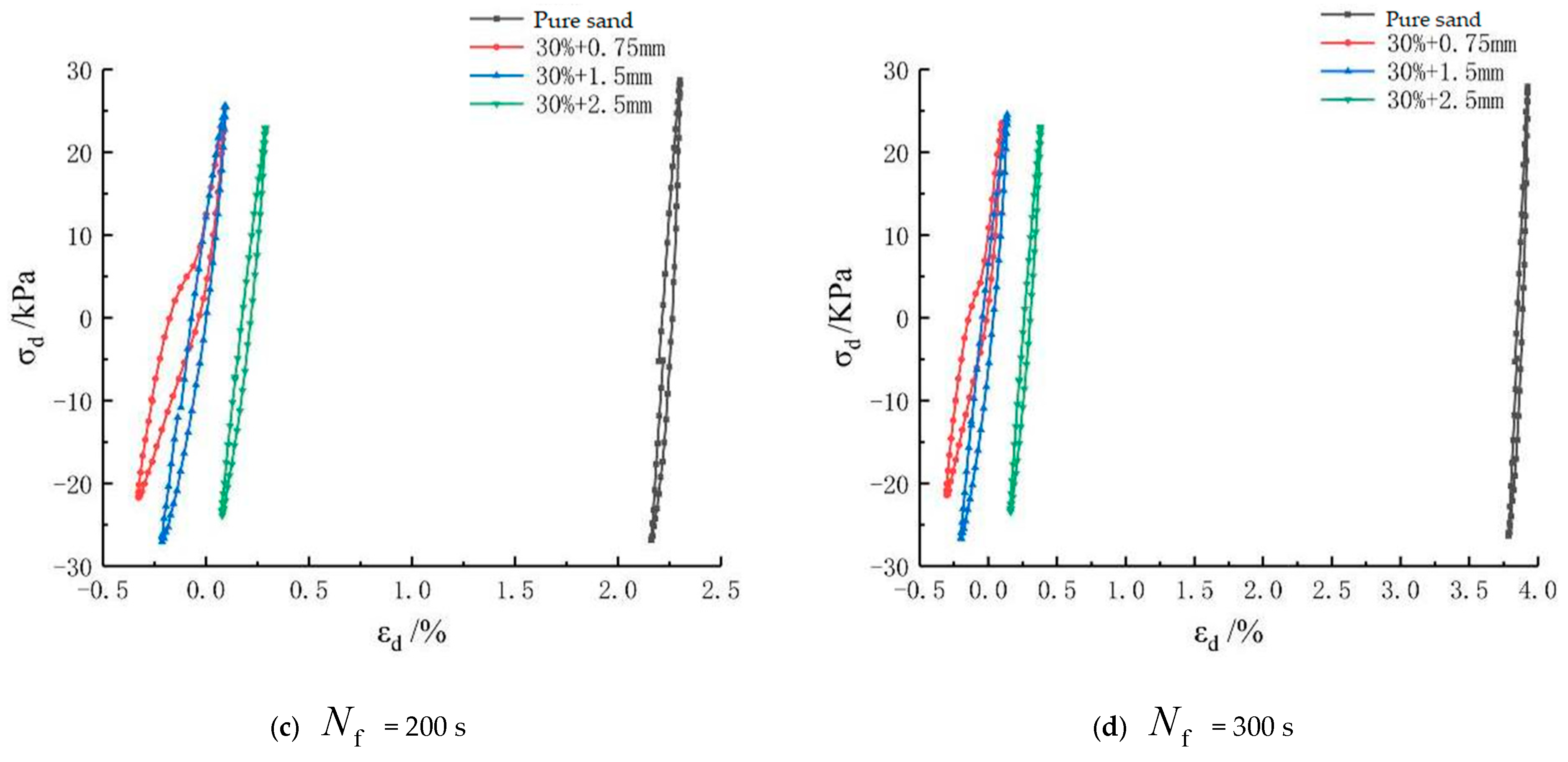
3.2. Change Rules of Hysteresis Curves under Graded Vibration Times

The dynamic stress–strain hysteresis curves of four times at 10 s, 100 s, 200 s, and 300 s under the cyclic loading were selected as shown in Figure 11, Figure 12 and Figure 13 below to more specifically study the dynamic stress–strain curve change rules of the rubber-particle-mixed-sand samples under cyclic loading. The developmental rule of the hysteresis curves of specified time was researched according to the hysteresis curve strain and the encircled area of each group of samples chosen at different times.

Figure 11a–d is the dynamic stress–strain hysteresis curves of the rubber-particle-mixed-sand samples in the three particle sizes under graded vibration times when the mixing amount of rubber $R_{\mathrm{f}}$ was 10%. The maximum strains of the samples mixed with 0.75 mm rubber particles achieved 0.73%, 0.95%, 0.97%, and 1.12%, respectively, under the cyclic loading at four times (10 s, 100 s, 200 s, and 300 s). The rubber-mixed sand samples in the size of 0.75 mm presented obvious softening under cyclic loading and the encircled area by the dynamic stress hysteresis curve decreased with the increase in vibration time, indicating a reduced energy consumption of the samples. The samples mixed with 1.5 mm rubber particles showed the maximum strains, namely 0.16%, 0.47%, 0.88%, and 1.27%, respectively, under cyclic loading at four times (10 s, 100 s, 200 s, and 300 s). The samples mixed with 2.5 mm rubber particles exhibited the maximum strains, namely 0.15%, 0.26%, 0.36%, and 0.51%, respectively, under cyclic loading at four times (10 s, 100 s, 200 s, and 300 s).

To further study the impacts of a 20% mixing amount of rubber particles on the stress–strain relationship curve, the hysteresis curves of various groups under graded vibration times are listed as shown in Figure 12. Specifically, the samples mixed with 0.75 mm rubber particles had the maximum strains, namely 0.02%, 0.14%, −0.24%, and −0.73%, respectively, under cyclic loading at four times (10 s, 100 s, 200 s, and 300 s), which presented a reciprocating strain form of tension and compression and did not produce a large cumulative strain. The samples mixed with 1.5 mm rubber particles reached the maximum strains, namely 0.06%, 0.27%, 0.87%, and 1.87%, respectively, under cyclic loading at four times (10 s, 100 s, 200 s, and 300 s), whose dynamic strain enlarged as the number of cycles increased and which generated a large cumulative strain. The samples mixed with 2.5 mm rubber particles reached the maximum strains, namely 0.04%, 0.13%, 0.33%, and 0.64%, respectively, under cyclic loading at four times (10 s, 100 s, 200 s, and 300 s), whose dynamic strain developmental rule was similar to that of the samples mixed with 1.5 mm rubber particles and whose dynamic strain was augmented with the increase in the number of cycles. Under 300 times of vibration, the latter only achieved a maximum strain of half of that of the former. Since rubber particles of large size possess a great energy absorption and vibration reducing performance, they could effectively decrease the strain of the samples under cyclic loading when mixed in the sand.

Furthermore, when the mixing amount of rubber particles was lifted to 30%, it could be seen from Figure 3, Figure 4 and Figure 5 that the samples primarily showed a reciprocating form of tension and compression. When the mixing rubber particle size was 0.75 mm, the maximum strains under cyclic loading at four times (10 s, 100 s, 200 s, and 300 s) were 0.16%, 0.21%, 0.08%, and 0.09%, respectively. When the mixing rubber particle size was 1.5 mm, the maximum strains under cyclic loading at four times (10 s, 100 s, 200 s, and 300 s) were 0.05%, 0.06%, 0.09%, and 0.13%, respectively. When the mixing rubber particle size was 2.5 mm, the maximum strains under cyclic loading at four times (10 s, 100 s, 200 s, and 300 s) were 0.14%, 0.23%, 0.29%, and 0.38%, respectively. As can be observed from the abovementioned three groups of data, as the mixing amount of rubber was 30%, the change in the samples under cyclic loading was mainly a reciprocating form of tension and compression, and prominent strain cumulation was not found in the samples. With a high mixing amount of rubber, the stressed skeleton inside the samples experienced a change in its form, which was dominated by the rubber particles, so the samples presented a reciprocating form of tension and compression under cyclic loading.

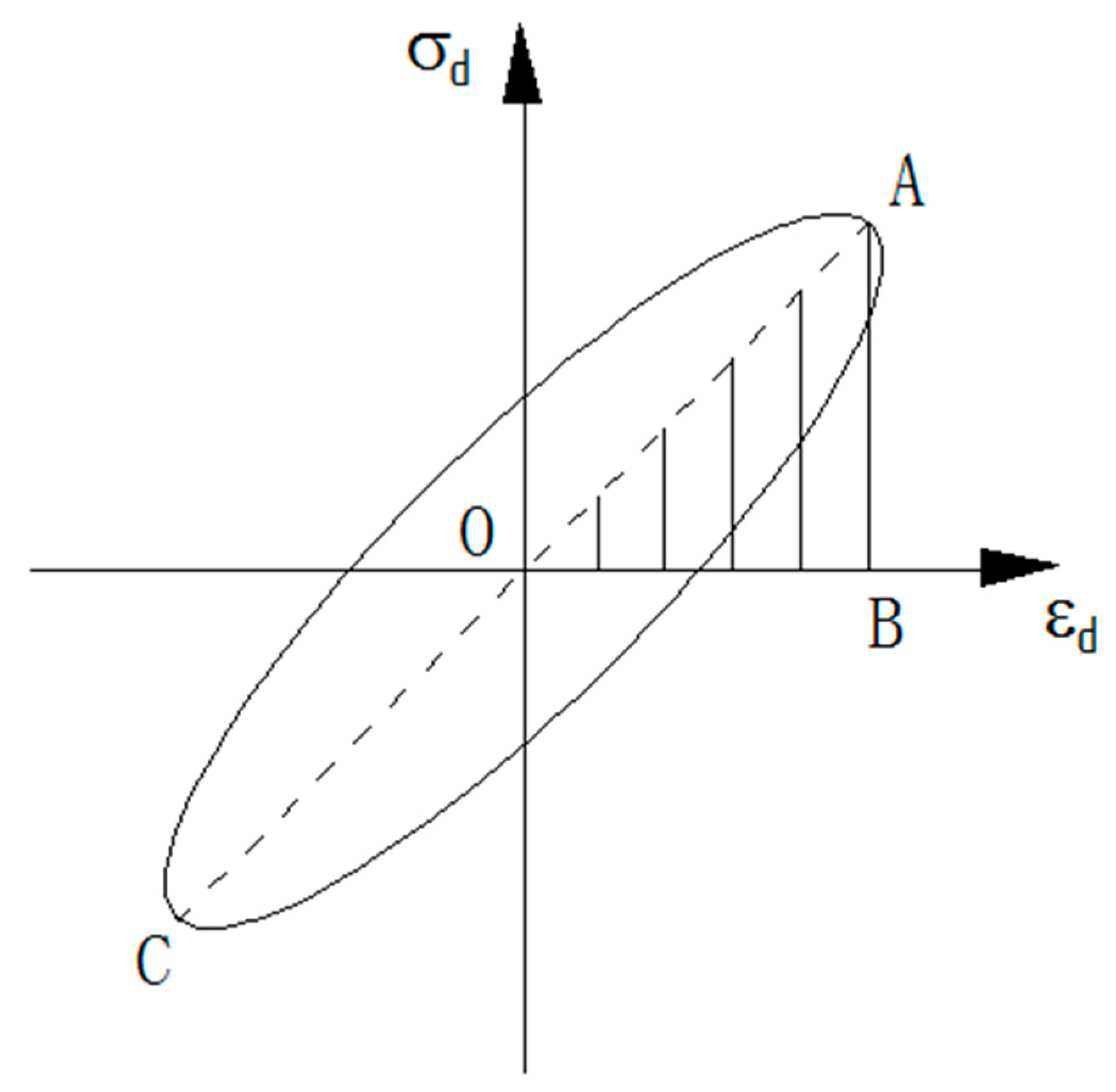
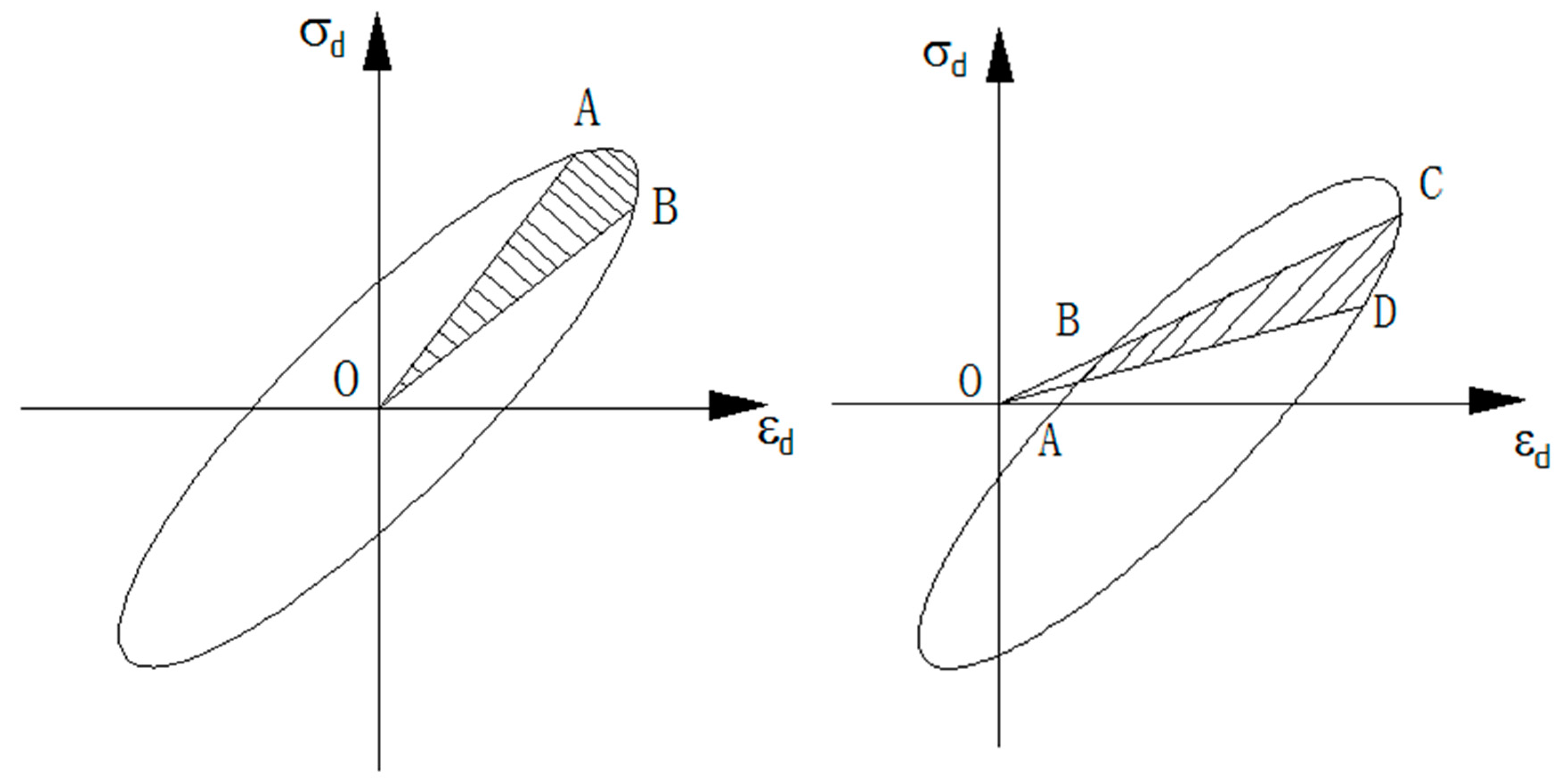
3.3. Change Rules of Dynamic Elastic Modulus and Damping Ratio of Hysteresis Curves

3.3.1. Change Rules of Dynamic Elastic Modulus

The hysteresis curve of the soil mass is the basis of studying the dynamic triaxial characteristics. The characteristic dynamic parameters of the soil mass, including the dynamic elastic modulus and the damping ratio, could be obtained by the quantitative characteristic analysis [14] of the hysteresis curves.

Figure 14 shows a standard dynamic stress–strain curve. A quantitative analysis of the hysteresis curve was conducted to gain the dynamic elastic modulus $E_{\mathrm{d}}$ and the damping ratio $\lambda$. The dynamic elastic modulus of the soil mass was calculated using the slope of the two endpoints A and C on the hysteresis curve in Figure 4, Figure 5 and Figure 6 according to Formula (4).

$$E_d=\frac{{\sigma }_{A\max }-{\sigma }_{C\min }}{{\epsilon }_{A\max }-{\epsilon }_{C\min }}$$

(4)

where: ${\sigma }_{A\max }$ and ${\sigma }_{C\min }$ denote the maximum value and the minimum value of the dynamic stress of the samples in each hysteresis curve, respectively.

${\epsilon }_{A\max }$ and ${\epsilon }_{C\min }$ denote the dynamic strain values, which correspond to the maximum value and the minimum value of the dynamic stress of the samples in each hysteresis curve, respectively.

Figure 15 displays a curve of the relationship between vibration time $N$ and dynamic elastic modulus $E_{\mathrm{d}}$ of the samples mixed with the rubber particles with different mixing amounts in different sizes. It was observed from the figure that the dynamic elastic modulus $E_{\mathrm{d}}$ of the pure sand samples and the samples with 20% and 30% mixing amounts of rubber R_f presented a decreasing trend with the increase in vibration time. When the mixing amount of rubber R_f was 30%, the dynamic elastic modulus of the mixed samples remained at a basically stable state as the vibration time increased. The dynamic elastic modulus $E_{\mathrm{d}}$ of all the rubber-mixed sand was smaller than that of the pure sand samples. Specifically, with a 10% mixing amount of rubber, the dynamic elastic modulus was reduced by 0.53 MPa (76%) compared with the pure sand samples to the greatest extent. With a 20% mixing amount of rubber, the dynamic elastic modulus was reduced by 0.49 MPa (70%) compared with that of the pure sand samples to the greatest extent. With a 30% mixing amount of rubber, the dynamic elastic modulus was reduced by 0.58 MPa (82.8%) compared with the pure sand samples to the greatest extent. After adding rubber particles to the pure sand, the samples had a decreased dynamic elastic modulus, illustrating that the sand mixed with rubber particles could reduce the shear stiffness of the soil mass, giving full play to the vibration resistance and reduction.

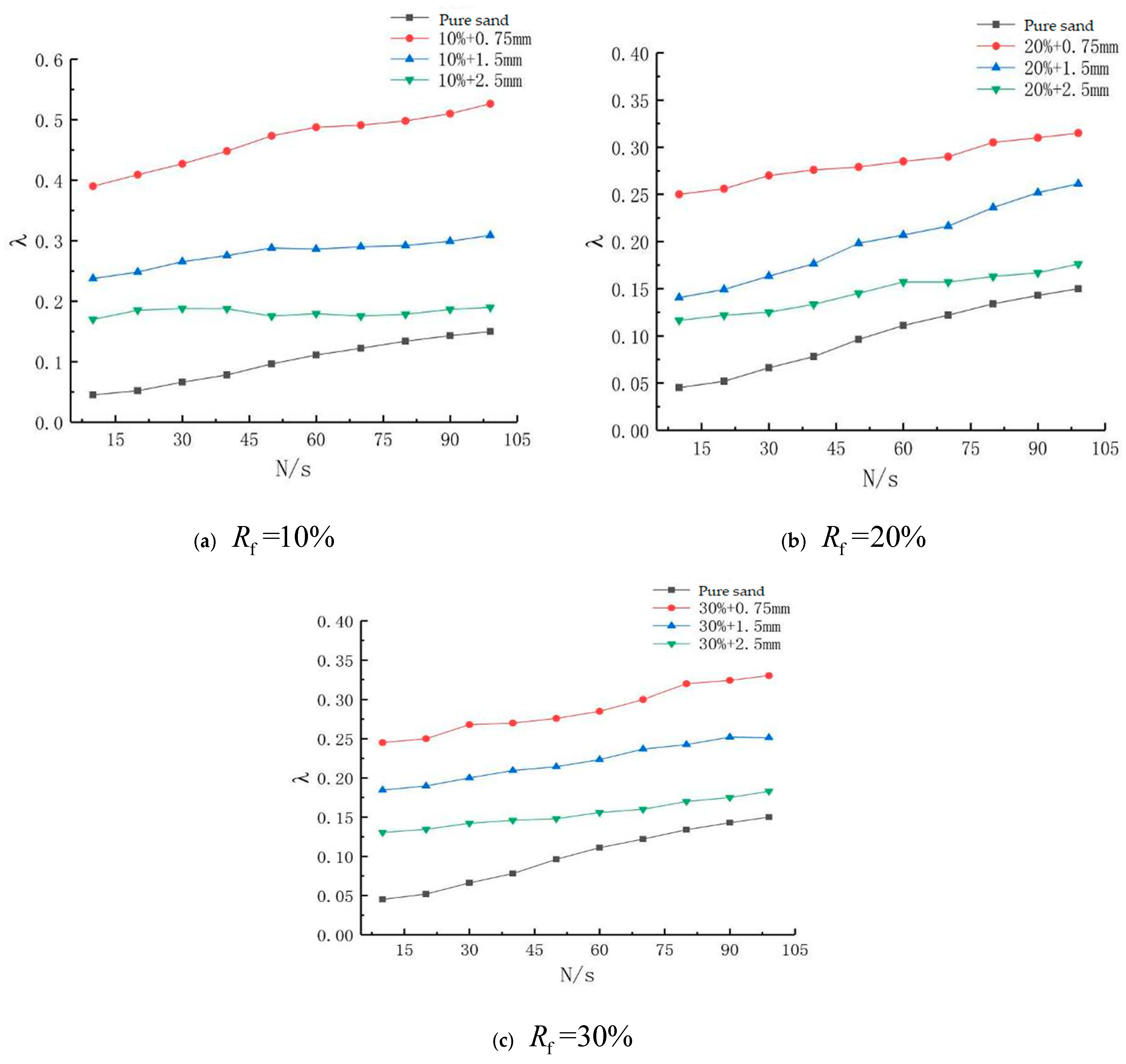
3.3.2. Change Rules of Damping Ratio

For geomaterials, the damping ratio of soil is one of the important parameters to reflect the dynamic characteristics of soil mass, which reveals the hysteresis of the dynamic stress–strain relationship of soil mass under cyclic loading.

At present, soil is regarded as a viscoelastic body to calculate the damping ratio, which is the ratio of the energy consumed to the total energy stored during a cycle of stress cyclic loading, and the calculation formula is shown in Figure 10.

$$\lambda =\frac{\Delta W}{4\pi W}$$

where: $\lambda$ refers to the damping ratio,

$\Delta W$ is the area of the hysteresis curve, representing the energy consumed in loading and unloading, and $W$ is the area of $\Delta OAB$, representing the total energy of loading and unloading.

The area encircled by the hysteresis curve needs to be accurately acquired for the calculation of the damping ratio. Currently, the most commonly used method is to fit the hysteresis curve using the elliptic curve. The calculated area of the ellipse is considered to be the area encircled by the hysteresis curve. However, the actual hysteresis curve is not a standard elliptic curve. Taking this test as an example, the GDS system was set to collect 50 data points in each vibration cycle, so the hysteresis curve was a curve formed by connecting 50 data points. Therefore, there were some errors in the method of fitting the stress–strain hysteresis curve with an elliptic curve, especially when the coincidence rate between the curve shape formed by connecting the test data points and the elliptic curve shape was low. In this case, the calculated damping ratio was quite different from the actual results. As a result, the polygon accumulation method proposed by Chen W [15] was applied to calculate the damping ratio in this paper. First, the stress–strain data points corresponding to the selected specific time were connected into a curve in sequence. At this time, the graph encircled by the curve was a polygon, and then the area of the hysteresis curve was obtained by calculating the polygon area.

In Figure 16, two points A and B are two adjacent data points. The OA side of the triangle was supposed as vector $a$ and the OB side as the vector $b$, and the area of the triangle encircled by the two vectors was half of the vector value of their cross product.

$$a\times b=\left|\begin{array}{cc}{a}_y& a_z\\ a_y& b_z\end{array}\right|i-\left|\begin{array}{cc}{a}_x& a_z\\ b_x& b_z\end{array}\right|j+\left|\begin{array}{cc}{a}_x& a_y\\ b_x& b_y\end{array}\right|k$$

(5)

$$S_{OAB}=\frac{1}{2}\left|OA\times OB\right|=-\frac{1}{2}\left|\begin{array}{cc}{\epsilon }_{ad}& {\sigma }_{ad}\\ {\epsilon }_{bd}& {\sigma }_{bd}\end{array}\right|$$

(6)

where: ${\epsilon }_{ad}$, ${\sigma }_{ad}$, ${\epsilon }_{bd}$, and ${\sigma }_{bd}$ mean the dynamic strain and dynamic stress, which correspond to the adjacent data points A and B in Figure 16.

Following the polygon accumulation method, the data in the GDS test recording system were utilized to calculate the area encircled by the hysteresis curve with Formula (7).

$$\Delta W=-\frac{1}{2}(\left|\begin{array}{cc}{\epsilon }_{1\mathrm{d}}& {\epsilon }_{1\mathrm{d}}\\ {\epsilon }_{1\mathrm{d}}& {\epsilon }_{1\mathrm{d}}\end{array}\right|+\left|\begin{array}{cc}{\epsilon }_{2\mathrm{d}}& {\epsilon }_{2\mathrm{d}}\\ {\epsilon }_{3\mathrm{d}}& {\epsilon }_{3\mathrm{d}}\end{array}\right|+\cdot \cdot \cdot +\left|\begin{array}{cc}{\epsilon }_{(\mathrm{n}-1)\mathrm{d}}& {\epsilon }_{(\mathrm{n}-1)\mathrm{d}}\\ {\epsilon }_{\mathrm{nd}}& {\epsilon }_{\mathrm{nd}}\end{array}\right|+\left|\begin{array}{cc}{\epsilon }_{\mathrm{nd}}& {\epsilon }_{\mathrm{nd}}\\ {\epsilon }_{1\mathrm{d}}& {\epsilon }_{1\mathrm{d}}\end{array}\right|)$$

(7)

where: ${\epsilon }_{nd}$ and ${\sigma }_{nd}$ represent the dynamic strain and dynamic stress corresponding to the adjacent data points in the hysteresis curve.

Figure 17 shows that the damping ratio of both the mixed sand samples and the pure sand samples exhibited an increasing trend as the vibration time grew and the damping ratio of the rubber-mixed sand samples was larger than that of the pure sand samples. With a 10% mixing amount of rubber, the damping ratio was augmented by 6.54 times to the maximum extent. With a 20% mixing amount of rubber, the damping ratio was augmented by 5.05 times to the maximum extent. With a 30% mixing amount of rubber, the damping ratio was augmented by 5.34 times to the maximum extent. Since the dry density ${\rho }_{\mathrm{d}}$ of all the samples was kept same in this test, the pore characteristics of the particles were the same. When the samples are mixed with rubber particles, energy absorption will occur on account of the elasticity of the rubber particles. Thus, the hysteresis of the soil mass is strengthened under cyclic loading. This was why the damping ratio of the rubber-mixed sand samples was greater than that of the pure sand samples.

4. Conclusions

The dynamic stress–strain hysteresis curve, dynamic elastic modulus, and damping ratio of saturated rubber-mixed sand samples were studied in this paper, and the conclusions were as follows:

(1) Under the same confining pressure and dynamic stress, the dynamic elastic modulus of the rubber-mixed sand samples was smaller than that of the pure sand samples. With a 30% mixing amount of rubber in the particle size of 0.75 mm, the dynamic elastic modulus of the samples showed a maximum decrease of 0.58 MPa. The sand mixed with rubber particles could decrease the shear stiffness of the soil mass, making full use of the vibration resistance and reduction. The behavior of sand became more ductile with an increasing granulated rubber content. Adding granulated rubber led to greater yielding strain and less tangent stiffness of the sand. The maximum dilation angle decreased with the decrease in granulated rubber content [16].

(2) Under the same confining pressure and dynamic stress, the damping ratio of the rubber-mixed sand samples was larger than that of the pure sand samples. When the samples were mixed with rubber particles, the rubber particles presented energy absorption because of their elasticity and thus the hysteresis of the soil mass was strengthened under cyclic loading. Therefore, the damping ratio of the rubber-mixed sand samples was greater than that of the pure sand samples.

(3) The sand samples mixed with rubber particles could prominently reduce the cumulative strain generated under the cyclic loading. When the mixing amount of rubber particles was large, the cumulative strain produced in the samples was far smaller than that of the pure sand samples. As rubber particles are featured by high resilience, they were regarded as stressed skeletons in the rubber-mixed sand with a high mixing amount to bear the external loading. At this moment, the strain produced due to the cyclic loading was a partially recoverable elastic strain, equivalent to adding a spring with recoverable strain in the pure sand samples. Hence, the cumulative strain generated in the samples under the cyclic loading was obviously decreased after adding rubber particles into the sand.

There were some limitations to this study. A study with larger sample size is required in future study. Moreover, a geotechnical engineer is required to check the particle size before prescribing a suitable quantity for the application of crumb rubber in the field.

References

1. Feng, Z.Y.; Sutter, K.G. Dynamic properties of granulated rubber-sand mixtures. Geotech. Test. J. 2000, 23, 338–344. [Google Scholar]
2. Pamukcu, S.; Akbulut, S. Thermoelastic enhancement of damping of sand using synthetic ground rubber. J. Geotech. Geoenviron. Eng. 2006, 132, 501–510. [Google Scholar] [CrossRef]
3. Senetakis, K.; Anastasiadis, A.; Pitilakis, K. Dynamic properties of dry sand/rubber (SRM) and gravel/rubber (GRM) mixtures in a wide range of shearing strain amplitudes. Soil Dyn. Earthq. Eng. 2012, 33, 38–53. [Google Scholar] [CrossRef]
4. Anastasiadis, A.; Senetakis, K.; Pitilakis, K. Small-strain shear modulus and damping ratio of sand-rubber and gravel-rubber mixtures. Geotech. Geol. Eng. 2012, 30, 363–382. [Google Scholar] [CrossRef]
5. Anastasiadis, A.; Senetakis, K.; Pitilakis, K.; Gargala, C.; Karakasi, I.; Edil, T. Dynamic behavior of sand/rubber mixtures. Part I: Effect of rubber content and duration of confinement on small-strain shear modulus and damping ratio. J. ASTM Int. 2011, 9, 1–17. [Google Scholar]
6. Senetakis, K.; Anastasiadis, A.; Pitilakis, K.; Souli, A.; Edil, T.; Dean, S.W. Dynamic behavior of sand/rubber mixtures, part II: Effect of rubber content on G/G0-γ-DT curves and volumetric threshold strain. J. ASTM Int. 2011, 9, 103711–103712. [Google Scholar] [CrossRef]
7. Sui, X.X. The Study on Seismic Isolation Performance of Granulated Rubber-Sand Mixture; Huanan University: Changsha, China, 2009. [Google Scholar]
8. Li, L.H.; Xiao, H.L.; Tang, H.M.; Hu, Q.Z.; Sun, M.J.; Sun, L. Dynamic properties variation of tire shred-soil mixtures. Rock Soil Mech. 2014, 35, 359–364. [Google Scholar]
9. Shang, S.-P.; Sui, X.-X.; Zhou, Z.-J.; Liu, F.-C.; Xiong, W. Study of dynamic shear modulus of granulated rubber-sand mixture. Rock Soil Mech. 2010, 31, 377–381. [Google Scholar]
10. Akbarimehr, D.; Eslami, A.; Aflaki, E. Geotechnical behaviour of clay soil mixed with rubber waste. J. Clean. Prod. 2020, 271, 122632. [Google Scholar] [CrossRef]
11. Mase, L.Z.; Likitlersuang, S.; Tobita, T. Cyclic behaviour and liquefaction resistance of Izumio sands in Osaka, Japan. Mar. Georesour. Geotechnol. 2018, 37, 765–774. [Google Scholar] [CrossRef]
12. Mase, L.Z. Shaking Table Test of Soil Liquefaction in Southern Yogyakarta. Int. J. Technol. 2017, 8, 747–760. [Google Scholar] [CrossRef]
13. Mojtahedzadeh, N.; Ghalandarzadeh, A.; Motamed, R. Experimental evaluation of dynamic characteristics of Firouzkooh sand using cyclic triaxial and bender element tests. Int. J. Civ. Eng. 2021, 20, 125–138. [Google Scholar] [CrossRef]
14. Cetin, H.; Söylemez, M. Soil-particle and pore orientations during drained and undrained shear of a cohesive sandy silt clay soil. Can. Geotech. J. 2004, 41, 1127–1138. [Google Scholar] [CrossRef]
15. Chen, W.; Kong, L.W.; Zhu, J.Q. A simple method to approximately determine the damping ratio of soils. Rock Soil Mech. 2007, 28 (Suppl. 1), 789–791. [Google Scholar]
16. Anvari, S.M.; Shooshpasha, I.; Kutanaei, S.S. Effect of granulated rubber on shear strength of fine-grained sand. J. Rock Mech. Geotech. Eng. 2017, 9, 936–944. [Google Scholar] [CrossRef]
Figure 1. The basic framework of the DYNTTS.
Coatings 12 01470 g001
Figure 2. Rubber particles of 0.75 mm.
Coatings 12 01470 g002
Figure 3. Rubber particles of 1.5 mm.
Coatings 12 01470 g003
Figure 4. Rubber particles of 2.5 mm.
Coatings 12 01470 g004
Figure 5. Sand used in the test.
Coatings 12 01470 g005
Figure 6. Installed sample.
Coatings 12 01470 g006
Figure 7. Pressure hood installed.
Coatings 12 01470 g007
Figure 8. Five-level loading curve back pressure.
Coatings 12 01470 g008
Figure 9. Dynamic stress–strain hysteresis curve.
Coatings 12 01470 g009
Figure 10. Relationship curve of mixed sand σ d - ε d with different rubber content. (a) R f = 0%, D r = 0%; (b) R f = 10%, D r = 0.75 mm; (c) R f = 10%, D r = 1.5 mm; (d) R f = 10%, D r = 2.5 mm; (e) R f = 20%, D r = 0.75 mm; (f) R f = 20%, D r = 1.5 mm; (g) R f = 20%, D r = 2.5 mm; (h) R f = 30%, D r = 0.75 mm; (i) R f = 30%, D r = 1.5 mm; (j) R f = 30%, D r = 2.5 mm.
Coatings 12 01470 g010aCoatings 12 01470 g010b
Figure 11. Dynamic stress–strain curve of a specified time ( R f = 10%. (a) Nf = 10 s; (b) Nf = 100 s; (c) Nf = 200 s; (d) Nf = 300 s.
Coatings 12 01470 g011aCoatings 12 01470 g011b
Figure 12. Dynamic stress–strain curve of a specified time ( R f = 20%). (a) N f = 10 s; (b) N f = 100 s; (c) N f = 200 s; (d) N f = 300 s.
Coatings 12 01470 g012
Figure 13. Dynamic stress–strain curve of a specified time ( R f = 30%). (a) N f = 10 s; (b) N f = 100 s; (c) N f = 200 s; (d) N f = 300 s.
Coatings 12 01470 g013aCoatings 12 01470 g013b
Figure 14. Standard dynamic stress–strain curve.
Coatings 12 01470 g014
Figure 15. Rubber-mixed sand elastic modulus with different rubber content and size. (a) Rf = 10%; (b)Rf = 10%; (c) Rf = 30%.
Coatings 12 01470 g015
Figure 16. Approximate calculation method of the dynamic stress–strain curve.
Coatings 12 01470 g016
Figure 17. Rubber-mixed sand damping ratio with different rubber content and size. (a) Rf = 10%; (b)Rf = 10%; (c) Rf = 30%.
Coatings 12 01470 g017