1. Introduction
Near Infrared Spectroscopy (NIR) can be an effective and fast tool for measuring objects with time-variable optical characteristics, e.g., plant-derived objects [
1,
2]. It can be a very effective tool for such analysis in combination with artificial neural networks. Digital Light Projection (DLP) spectroscopy utilizes modern solutions in the scope of measuring light reflection and absorption spectra. A key solution is the application of a Digital Micromirror Device (DMD), which replaces the system of detectors or scanning mechanism and acts as a programmable wavelength filter [
3]. In practice, the advantages of this solution are miniaturization, very high mobility and autonomy of instruments, high sensitivity, low signal-to-noise ratio, the universality of measurements, and programmability of measuring instruments and systems for final processing of measurement results. The short time of a single-spectrum measurement makes it possible to quickly obtain measurement results of reflectance spectra of various objects, including those rapidly changing over time outside of a laboratory.
The beginnings of scientific interest in Artificial Neural Networks (ANNs) reaches the 40s of the twentieth century. Since then, many different types of ANNs and their applications have been developed. Probably one of the most popular ANN applications concerns optimization. In the paper [
4], a novel hybrid ANN was presented to optimize the grit-blasting process to improve thermal spraying coatings’ structural properties and corrosion-resistance performance. A similar application of ANNs was included in [
5]; i.e., a backward propagation neural network was applied to efficiently optimize the pulse electrodeposition process of Ni–W-graded coating. Another example of using ANNs in materials science was described in the paper [
6]. In that case, ANNs were used not for optimization but for prediction; i.e., a back-propagational artificial neural network was proposed to predict the hot deformation behavior of superalloy nimonic 80A. The ANNs were trained and verified based on the experimental data from isothermal compression tests. In addition to optimization and prediction, ANNs are also used in classification problems. In the article [
7], a classification method for four types of carbon fiber fabrics was proposed using ANNs and Support Vector Machine (SVM) based on 229 experimental data groups. A slightly different example is included in the article [
8] concerning the maritime area of interest. In this paper, the possibility of applying an ANN to evaluate added resistance in waves at the different sea states that the ship will encounter during navigation was investigated. As it can be seen, many various examples of using ANNs can be found in different technology areas. Therefore, ANN was also proposed to determine the aging time of plants, i.e., the problem formulated in this paper.
The main goal of this paper is to expand methods of analyzing the reflectance spectra of objects with properties changing over time using the DLP measuring technique. Based on conceptions of applications’ expert systems developed to establish input-output relationships of various manufacturing processes and data analysis [
4,
9,
10,
11], a method to analyze time-variable optical reflectance spectra in DLP spectroscopy using ANN has been applied.
In the next section, the designed and implemented apparatus and method are described. Then, details about tested objects and used ANNs with training methods are presented. In the end, a discussion on obtained research results and a summary with main conclusions and a plan of future research are included.
2. Measuring Apparatus and Method
The DLP NIRSCAN NANO device, a compact spectrometer from Texas Instruments (Dallas, TX, USA), operating in the wavelength band from 900 to 1700 nm, was used to record spectra. Its dimensions, 58 mm × 62 mm × 36 mm, and the absence of an external power source make it possible to perform mobile spectra measurements [
12]. The device works in reflectance mode. Reflectance (
R) is the ratio between the intensity of light reflected from the sample (
I) to the intensity of reflected background light or reflected from a reference surface (
Ir) [
13]:
The main advantage of the device is its mobility and capability of performing measurements under various conditions.
The standard software, compatible with a PC running on a Windows operating system, enables registration, acquisition, and data visualization. It is possible to control the device using a mobile application via the Bluetooth standard. The spectrometer can register 228 measurement points in the wavelength band from 900 to 1700 nm within 2.63 s, repeating the measurement six times for every point, then calculating the mean for the given point. The result is presented in a dialog window of the software in the form of a chart or file in DAT or CSV format. The number of scans can be changed, which directly influences the time of measurement.
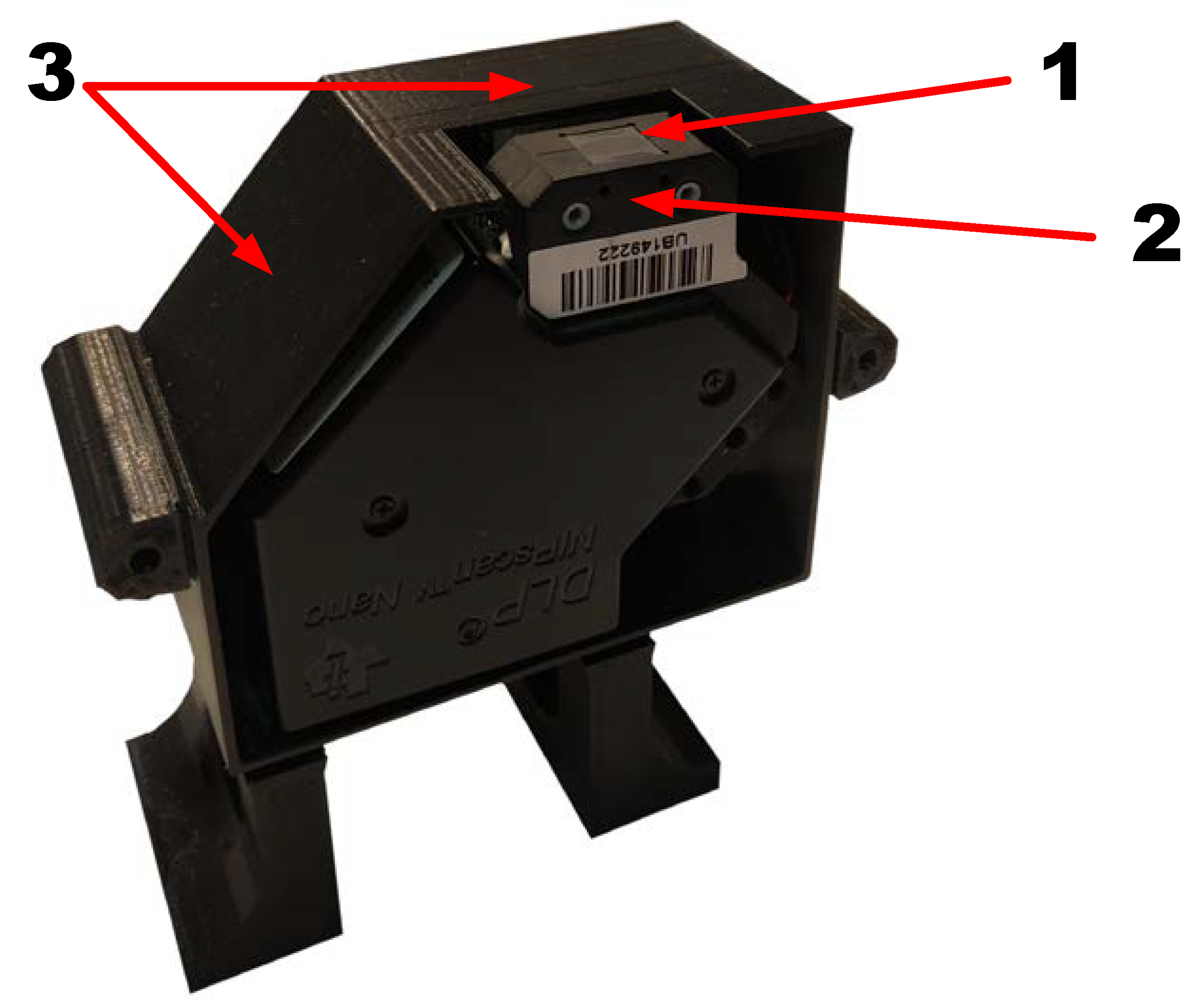
Figure 1 presents the principle of the device’s operation and how it performs measurements. The sample situated near the spectrometer’s window is illuminated by two light sources in the form of lightbulbs controlled by the device’s controller. The reflectance spectrum of the lightbulbs from the reference surface is known and saved in the device’s memory. Depending on the tested object, a specific part of the light is absorbed by the sample, a certain amount is scattered, and a part of the light is reflected off of the object’s surface into the slit of the device. Further on, the light goes to the optical system in the process, where it is split by a diffraction grating and directed by a lens to the DMD micro-mirror array, which directs the light in a particular sequence to the detector, where it is processed into an analog signal [
3]. The design of the device is shown in
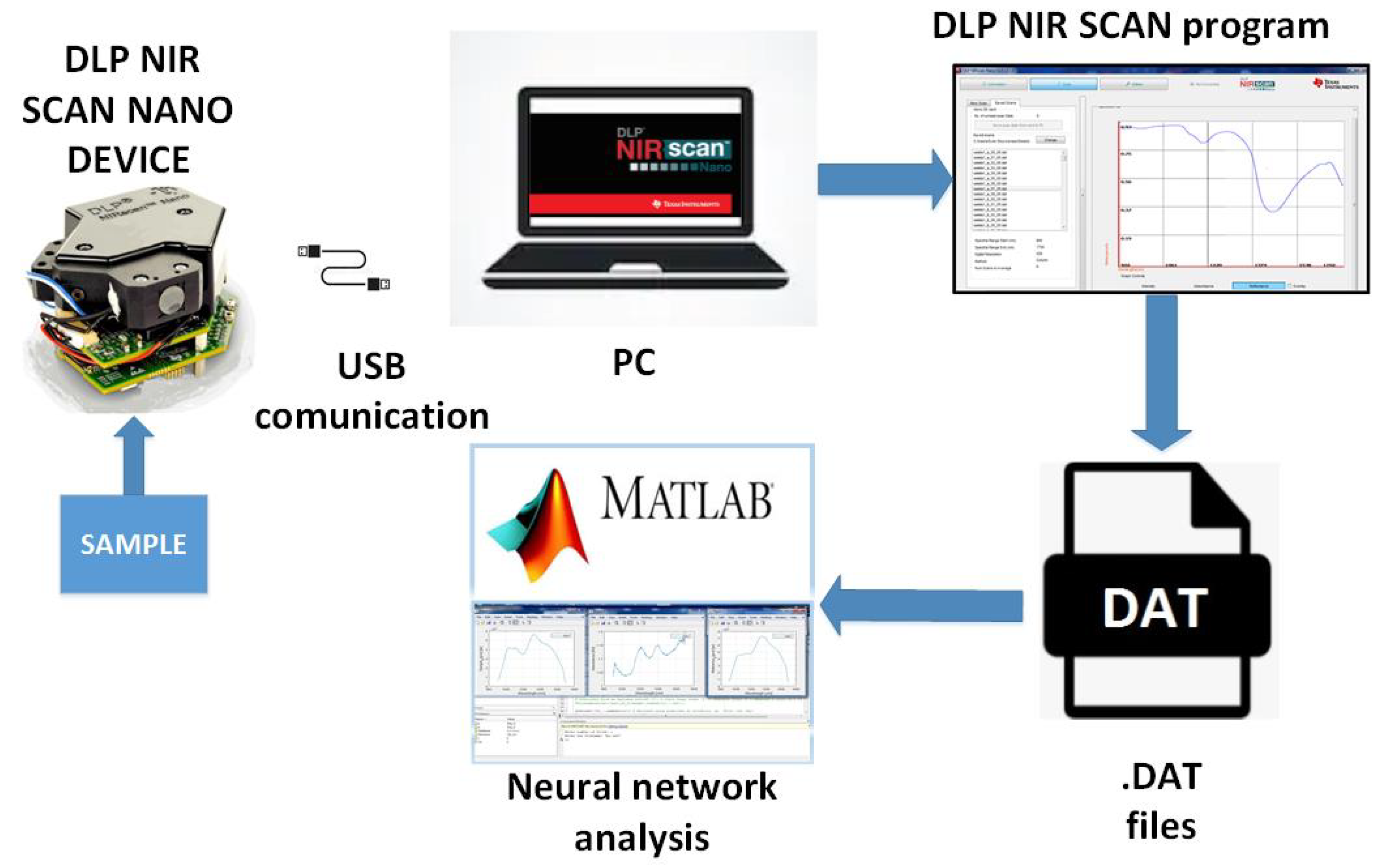
Figure 2. The scheme of measurement data flow and view of the test stand were shown on
Figure 3 and
Figure 4 respectively.
3. Tested Objects
The criterion for selecting objects was the variability of their optical characteristics in the time domain for several, ten or so, or tens of minutes. Biological materials, mainly the leaves of plants, were chosen as the test subjects, as the process of their aging over time is spectroscopically measurable. It is also an interesting group of objects because analysis of the aging process and the determination of freshness may be helpful in processing, transportation, and commerce. Each tested organic object has a characteristic range or several ranges in the reflectance spectrum where changes are the most visible. For plants having green leaves, this is typically the interval from 1400 to 1500 nm. In this light wavelength interval, significant changes occur in the measured reflectance value (as time passes, this value drops within the range mentioned above, pertaining to green plants (
Figure 5)). This phenomenon may be caused by water absorption within this range. As the leaf withers, the level of moisture in the sample changes, which directly influences the reflectance value at the given time of measurement [
13,
14,
15].
Substantive analysis of the internal processes in objects of plant origin causing these changes is not the goal of this paper. The transformation of spectra of specific objects in the time domain has been presented to specify the nature of the test dataset, acquired for measurements using the DLP technique, which may be helpful in processes of controlling objects during ware-housing, processing, and storage of various products of plant origin. As part of this research, it was determined that measuring conditions and settings that are not entirely stabilized in testing conditions employing the primarily mobile, portable DLP device; e.g., distance from sample and background light, angle of the tested object’s surface relative to the surface near the DLP’s inlet window, and curvature (roughness, non-flatness) of the tested object’s surface, may influence measurement results (mean signal value, repeatability, and even details of the spectrum). The above potential measurement uncertainties are why artificial neural networks were applied to analyze measurement data. However, the main objective of using artificial neural networks is to learn measurement series to identify random samples in the future and determine their aging process in a given instant based on a previously obtained reference series of measurements, which has been identified and processed by the artificial neural network.
4. Application of Artificial Neural Networks
Unidirectional ANNs were built using Matlab software and then trained using various types of the following training methods available in the Neural Network Toolbox [
16]: trainbr, trainlm, trainbfg, traincgb, traincgf, traincgp, traingda, traingdm, traingdx, trainrp, and trainscg. All of these functions have the appropriate mathematical names available in
Table 1. These one-direction networks use reversal error propagation. The network consisted of a layer containing hidden neurons, the number of which was changed. The following structure was the output layer, where the network was tested. The entire measurement series, containing spectra and information about their measurement time, were given on the network’s input. The mean-squared error of measurement time was obtained on the network’s output. The number of neurons in the hidden layer was changed in the constructed networks. The tested objects were leaves of individual green plants–their aging process, and the method of describing this process using neural networks trained with different available methods was chosen in order to be able in the future to select the optimal network training method to identify random samples. It was also checked how the number of hidden neurons, ranging from 10 to 200 with a value step of 10, influences the change of the network’s output parameter [
17], i.e., allows for minimization of the Mean Squared Error (MSE) of sample measurement time, with a relatively short network training time. As the number of neurons increased, the result was not always burdened by a lower error (this depends on the method). However, the training time of the neural network was permanently extended. Testing of objects (leaves) using the spectrometer lasted, depending on the object, from 6 h to 12:30 h with a differing time resolution (15 min or 30 min), with the measurement being repeated five times within the given time interval (the duration of a single measurement was 2.63 s).
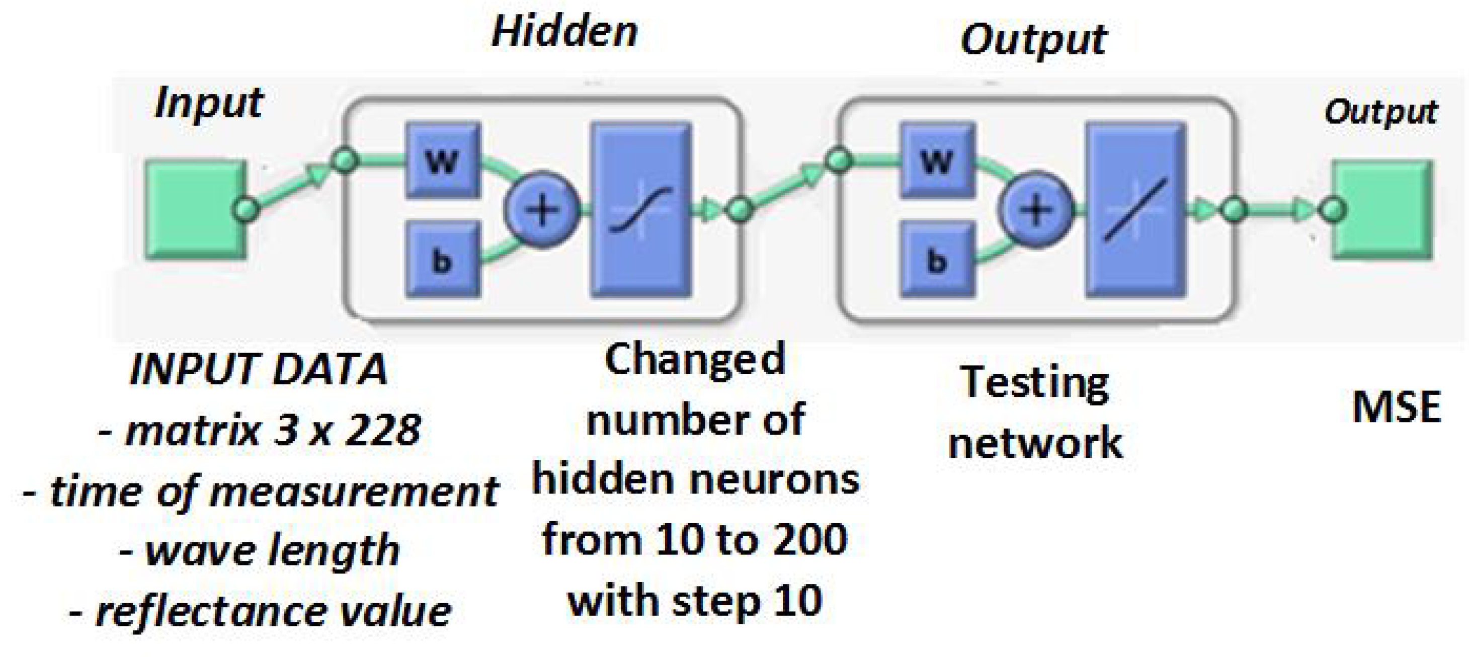
In
Figure 6, the architecture of ANN implemented in Matlab is visualized. The input data refer to the time and spectrum of the examined objects. At the network’s output, MSE is obtained for a specific learning method with a particular number of neurons in the hidden layer. A total of 80% of the measurement data was used to train the network, and 20% was used to test the network.
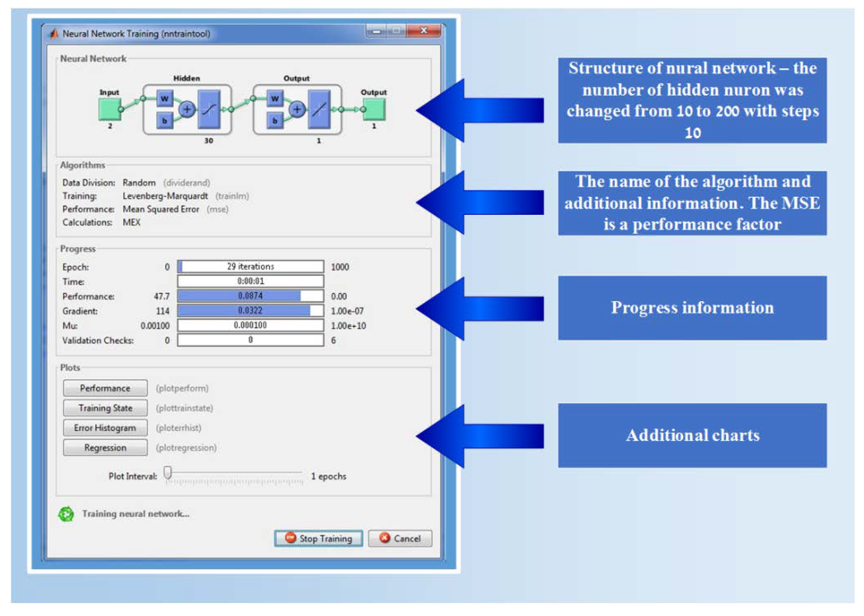
The software controlling the spectrometer recorded spectra in CSV or DAT files. However, the file names had to be input into the software by the operator appropriately so that the information about the time of measurement was known. For example, in the case of the common dandelion leaf object, the file name was “1_00-30.csv,” meaning that this was the first measurement in the 30th minute from the start of the sample testing process. Next, the measurement series containing spectra from the entire testing interval was loaded into Matlab software for “training” the network using available training methods to find the best training method, allowing for the greatest accuracy of sample aging time detection within the shortest time. The artificial neural network’s training program window is presented in
Figure 7. The options available in this window enables to plot the following plots:
“Performance” chart, illustrating the changes of the MSE value in the following iterations;
“Training State,” showing additional parameters describing the network;
“Error Histogram,” presenting the MSE error changes depending on iteration leaves; and
“Regression” chart, visualizing the variability of regression with successive iterations.
The program carried out 1000 iterations for every training method, and the network’s learning and testing times are described using the Time parameter. The Performance parameter is the most important in the neural network learning and testing, directly addressing the MSE, which translates to the network’s goodness of fit. The lower the MSE value of sample measurement time, the better the neural network has learned and tested the given measurement series. Moreover, the identification of a random sample will be more effective. Supposing the measurement series is burdened by significant measuring errors, the MSE of measurement time increases. In that case, the network learns and tests the given series ineffectively, and analysis is extended over time.
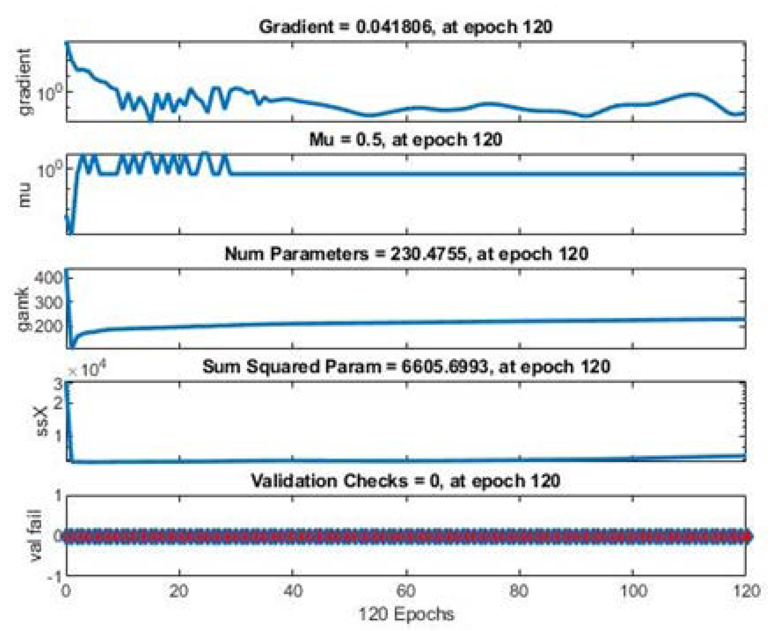
The graphs created by the Neural Network Training Matlab tool are presented below in
Figure 8,
Figure 9,
Figure 10 and
Figure 11. Such charts are created dynamically in the program during the following iterations depending on the method and the number of hidden neurons in the network. It would be challenging to present all the graphs for each number of neurons depending on the method and each object separately. Therefore, the charts for selected moments of the learning process have been visualized. For instance, the change of MSE from the beginning to the 299th epoch is presented in
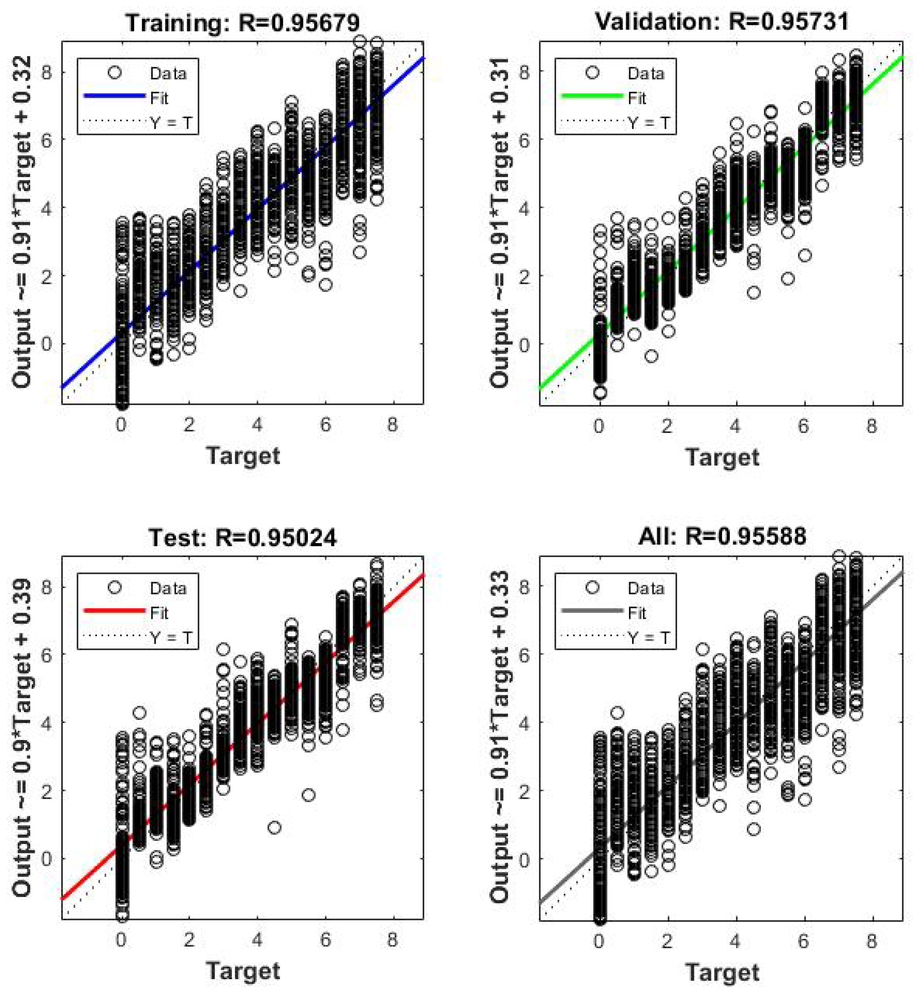
Figure 8. As it can be seen, the most significant changes in MSE are observed for the first 100 epochs. In
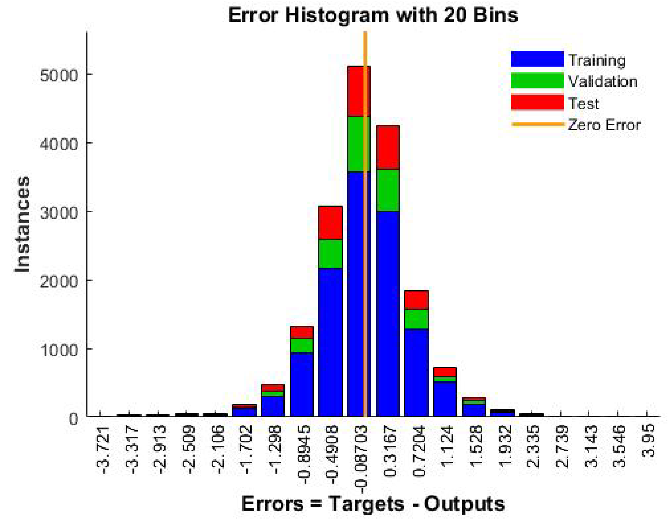
Figure 9, the regression charts obtained from the Neural Network Training tool are presented. The regression results can be seen for the particular processes: Training, Validation, Test, and total regression (chart entitled “All”). Outstanding regression analysis results were received, i.e., the value of the R parameter higher than 0.9. In the end, the error histogram is presented in
Figure 10.
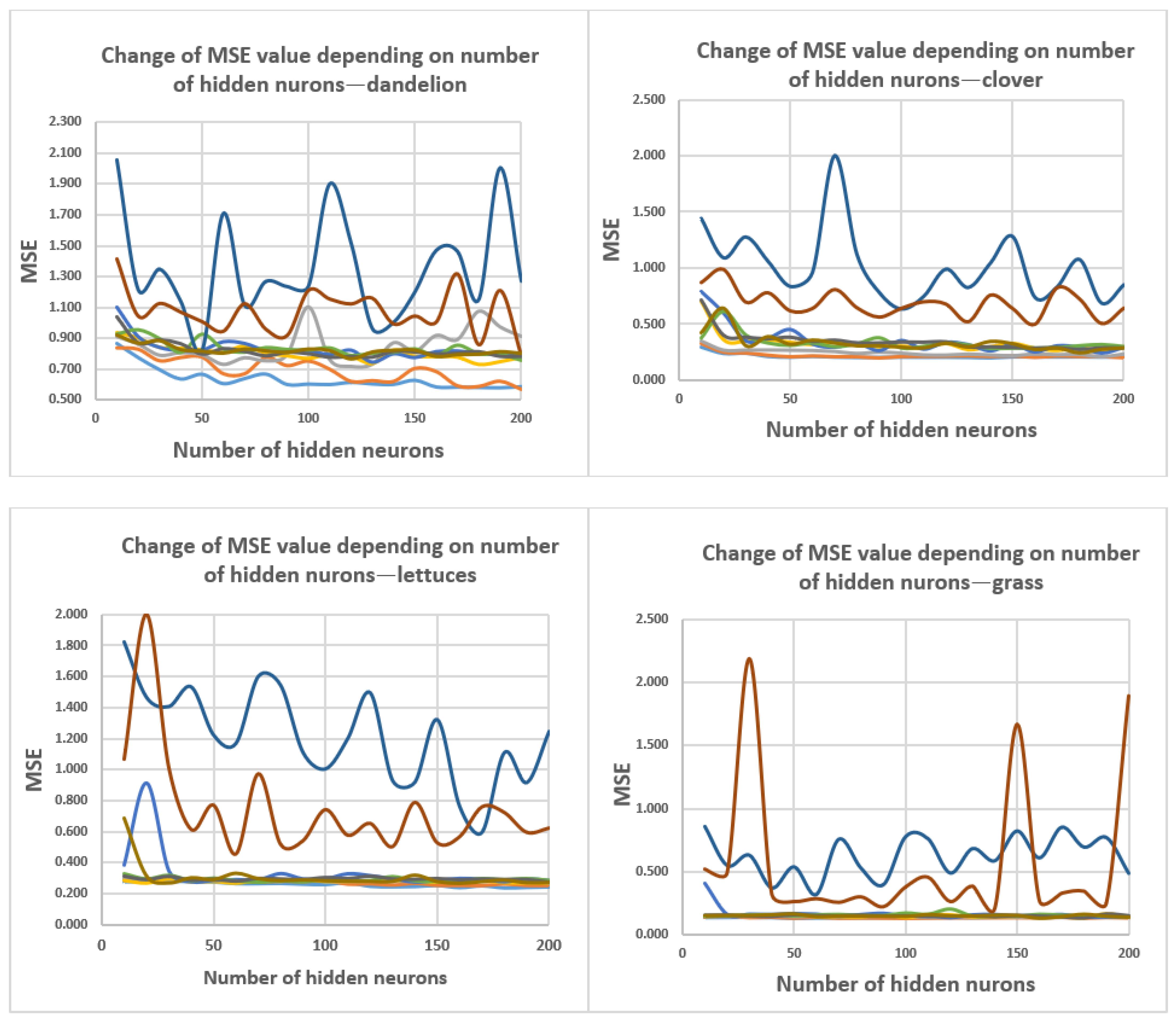
During the research, the eleven neural network learning methods were tested using 76 measurement spectra of the standard dandelion leaf. The results are presented in a chart (
Figure 12), which illustrates the final progression of the MSE result of a network with given parameters. Additionally, the minimum MSE values for the appropriate number of neurons in the hidden layer are shown in
Table 2.
The least effective network learning method for all the objects (dandelion, clover, lettuce, and grass) was the traingdm method, i.e., the least descent algorithm, where the weights are updated in the direction of the negative vector of the error function’s gradient. The traingdm algorithm is where the descent step is modified by a “momentum” factor allowing the network to avoid local minimum traps [
18]. Results of this learning method deviated substantially from those of the other methods, and for this reason, it was rejected and not shown on the charts. It also turns out that two methods of learning differ significantly in terms of the size of MSE and are not as effective as the others—the traingdx and traingda methods.
Using the Bayesian regularization backpropagation (the trainbr method) allows obtaining the best results for all the examined objects. Almost similar results were achieved using trainlm method, i.e., the Levenberg–Marquardt optimization. For instance, the clover object obtained the MSE equal to 0.205 for the neural network with only 50 hidden neurons. The improvement of this result to the level of 0.199 was achieved for the network with 140 hidden neurons. Similarly, analyzed grass spectra for this method obtained the MSE level of 0.134 for the ANN with 50 hidden neurons. The worst results were received for the dandelion object, which reached the MSE level equal to 0.637 for the network with 40 hidden neurons. For the most extensive calculation time, i.e., the network with 200 hidden neurons, dandelion obtained the MSE equal to 0.568.
5. Summary
Since the second half of the 20th century, the NIR technique has been developing very rapidly, as indicated by the scientific community’s interest in this subject matter. Increasingly advanced instruments are becoming available, and their overall dimensions are decreasing, making it possible to perform measurements of spectra of various objects outside of the laboratory (mobile measurements).
The measurement process combined with the analysis of spectra using ANNs may be an effective tool for different analyses, e.g., determination of leaf ageing as it was proved in the paper. Selection of the most effective ANN’s training methods carried out in the results of comparison tests may be helpful in further study as well as for other researchers. It should help reduce the time for the complete analysis by, e.g., minimization of the number of neurons in the network’s hidden layer. Moreover, it can also contribute to the decrease of over parametrization risk. It is also possible that not every method may be appropriate for the given group of objects.
The results of the above study may have significance in determining the quality or freshness of plant products or identifying and classifying objects. The technique of identifying and classifying the properties of objects may be successfully applied in the food industry and in various types of production lines, where there is a need for different analyses, e.g., classification.
The method and results of the presented research are concerned with the analysis of the optical reflection spectrum of thin near-surface layers. The applied method of data analysis can be treated as universal and applied to any object, including any layers applied to the surface. The objects measured in this particular case are only model objects with non-stable optical properties, mainly reflectance.


