Optimization through the Levenberg—Marquardt Backpropagation Method for a Magnetohydrodynamic Squeezing Flow System

Abstract

The present study introduced the unsteady squeezing flow of two-dimensional viscous fluid with nanoparticles between two disks by using the Levenberg–Marquardt backpropagated neural network (LMB-NN). Conversion of the partial differential equations (PDEs) into equivalent ordinary differential equations (ODEs) is performed by suitable similarity transformation. The data collection for suggested (LMB-NN) is made for various magnetohydrodynamic squeezing flow (MHDSF) scenarios in terms of the squeezing parameter, Prandtl number, Brownian motion parameter, and the thermophoresis parameter by employing the Runge–Kutta technique with the help of Mathematica software. The worth of the proposed methodology has been established for the proposed solver (LMB-NN) with different scenarios and cases, and the outcomes are compared through the effectiveness and reliability of mean square error (MSE) for the squeezing flow problem MHDSF. Moreover, the state transition, Fitness outline, histogram error, and regression presentation also endorse the strength and reliability of the solver LMB-NN. The high convergence between the reference solutions and the solutions obtained by incorporating the efficacy of a designed solver LMB-NN indicates the strength of the proposed methodology, where the accuracy level is achieved in the ranges from 10${}^{-6}$ to ${10}^{-12}$.

1. Introduction

The flow between two moving parallel plates toward each other is called squeezing flow. Recently, scientists and engineers have been interested in related research with squeezing flow due to its valuable use in industries like liquid metals, injection shaping, lubrication, food, and polymer processing. Stefan [1] reported the first paper authored on the squeezing flow under lubrication approximation. Studies continued on the same problem, and, in 1886, Rooynolds [2] presented a solution for elliptic plates, in particular. Atlas et al. [3] developed a numerical solution for unsteady nanofluid flows between two parallel plates using the finite difference method. Domairry and Hatami [4] investigated squeezing Cu-Water nanofluid flow using a differential transformation method (DTM). Domairry and Aziz [5] studied magneto-hydrodynamic (MHDSF) between two parallel disks with effects such as suction or injection of the fluid by implementing the homotopy perturbation method (HPM).

To improve energy transfer fluids’ thermal conductivity, scientists immersed nanoparticles in the basic fluids, creating a new type of fluid known as nanofluid. This fluid type is considered important as it enters into many modern applications due to these fluids’ new properties. Magnetic nanofluids will likely have a significant role in the future in cancer treatment and directing particles in the bloodstream. Buongiorno [6] studied the thermal properties of base fluids by improving the mathematical model containing the effects of Brownian motion and thermophoresis. Khan and Pop [7] used the Keller-box method to analyze nanofluid’s two-dimensional flow over a linearly stretching surface. Turkyilmazoglu [8] investigated the transfer effect of heat and mass on MHD flow based on slip conditions and different kinds of nanoparticles. More studies for nanofluids in various dimensions are cited [9,10,11,12,13,14].

The aforementioned numerical methods that are used to solve various problems have merits and demerits. Therefore, a stochastic computing system is discovered to find answers to complicated nonlinear problems, and, despite this, it was only entered quickly to solve the squeezing flow model’s governing system. The stochastic computing solvers benefit from computing through artificial neural networks (ANN) systems and its improvement in answering complicated problems in terms of the system of ordinary or partial equations.

Stochastic numerical computing solvers have many different applications in numerous domains and areas, for example, plasma physics [15], finance models [16,17], the mechanics of fluid [18,19,20,21], the different system of pantograph and Emden–Fowler equations [22,23,24,25], biological studies [26,27,28], mosquito dispersal model [29], and studies of atomic physics [30]. Some more recent research work related to the soft computing paradigms for the different fluid flow systems under the impacts of heat transfer and magnetohydrodynamics is also provided in the references [31,32,33]. The structure of our treatment is illustrated as follows:

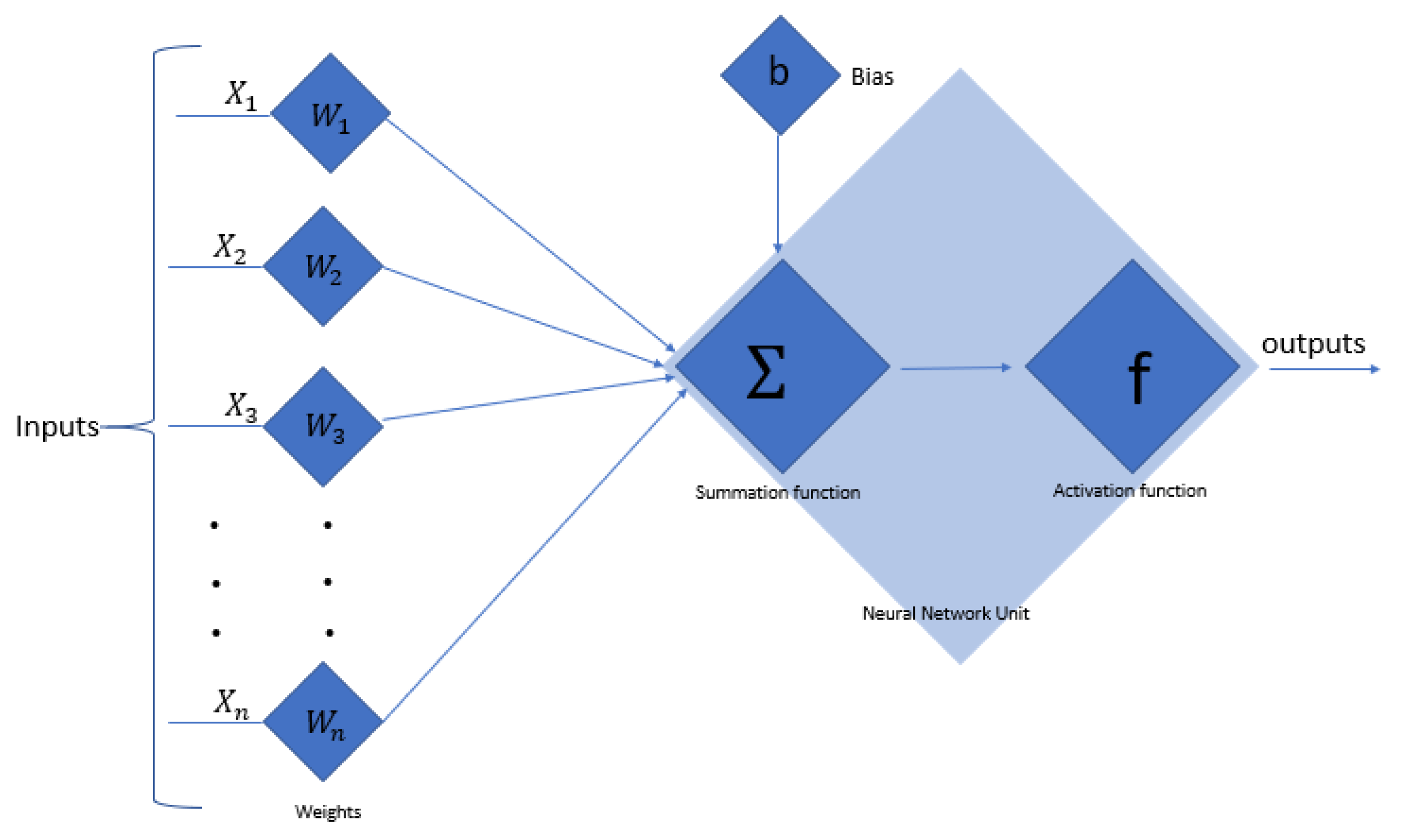
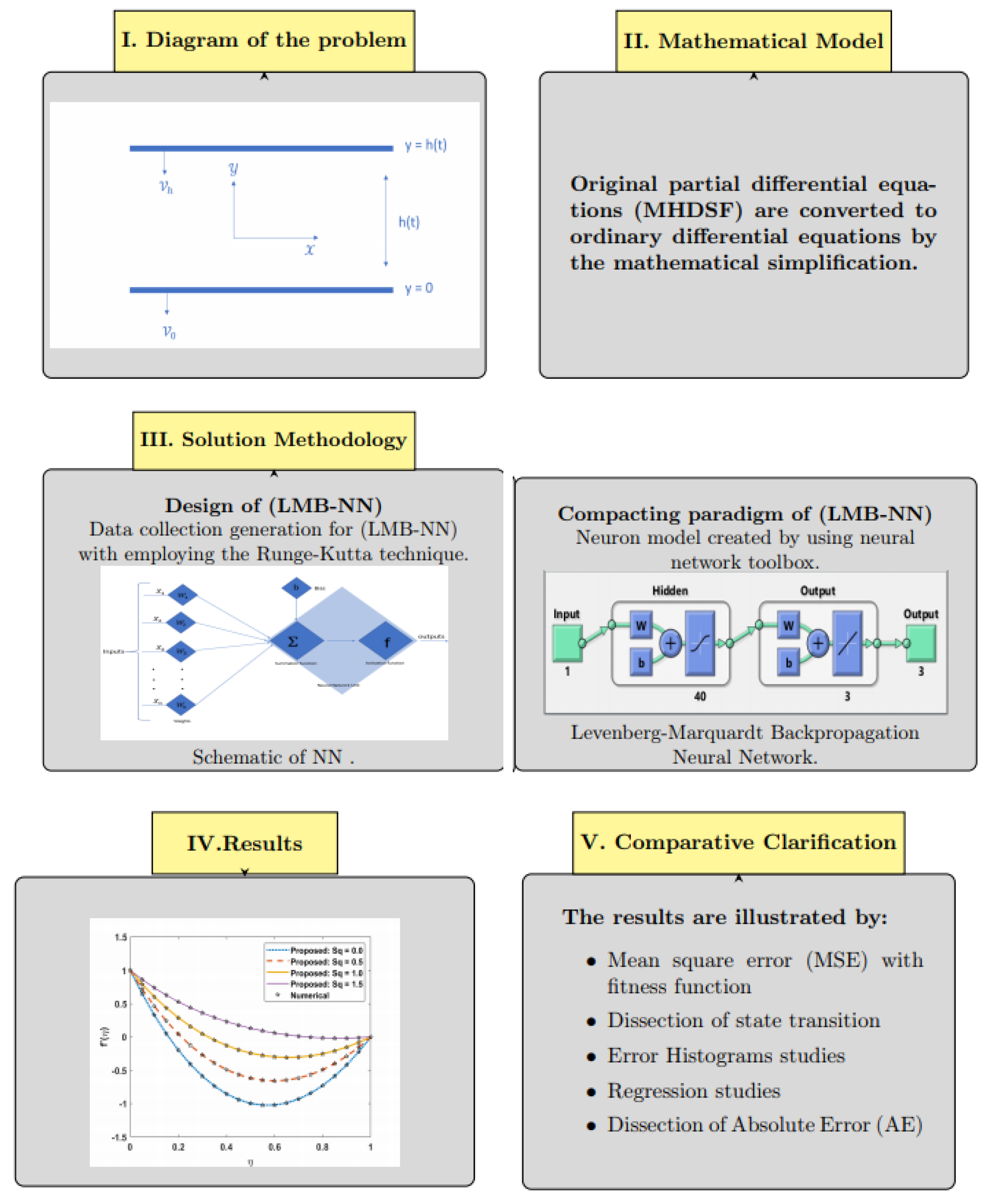
• A soft computing technique-based Levenberg–Marquardt algorithm is used to solve the fluid flow problem MHDSF.
• Mathematical simplification is presented for MHDSF in terms of partial differential equations to be easier in dealing with the proposed model (LMB-NN).
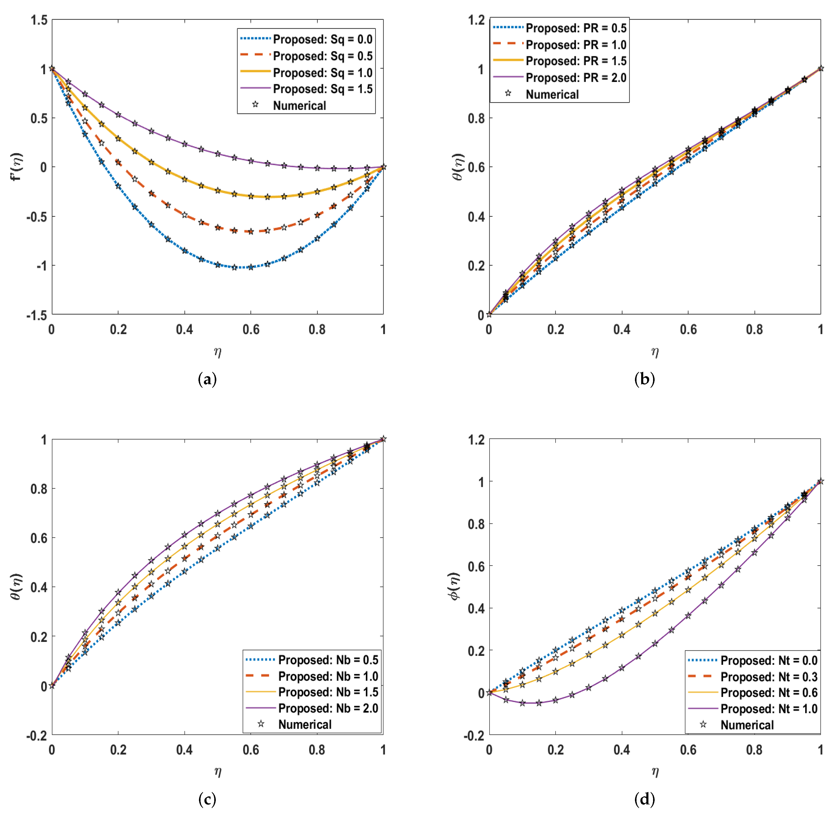
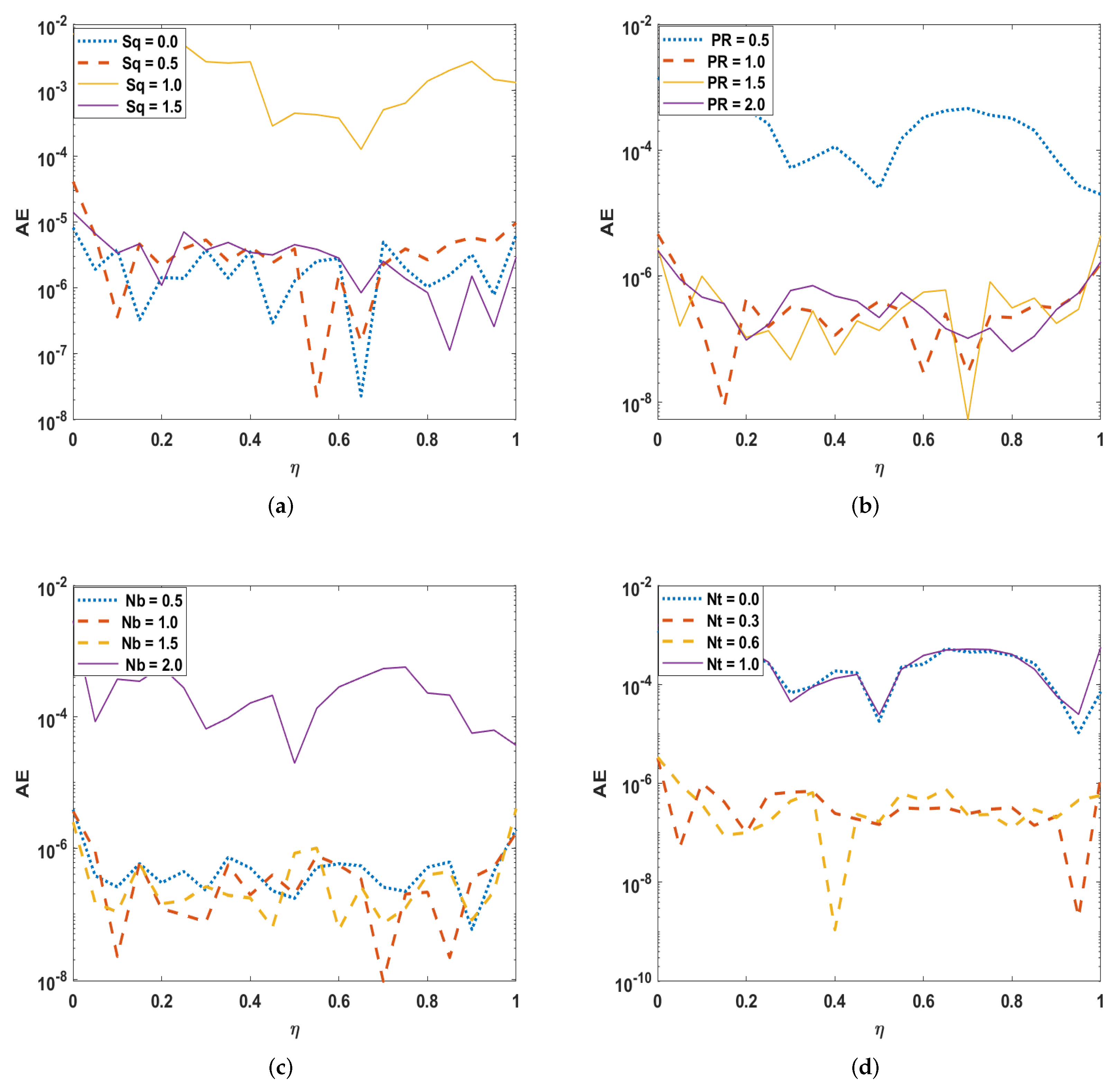
• Creation of the data set for a suggested (LMB-NN) based on squeezing parameter, Prandtl number, Brownian motion parameter, and thermophoresis parameter is used in solution (MHDSF) by employing the Runge–Kutta technique for various scenarios and cases.
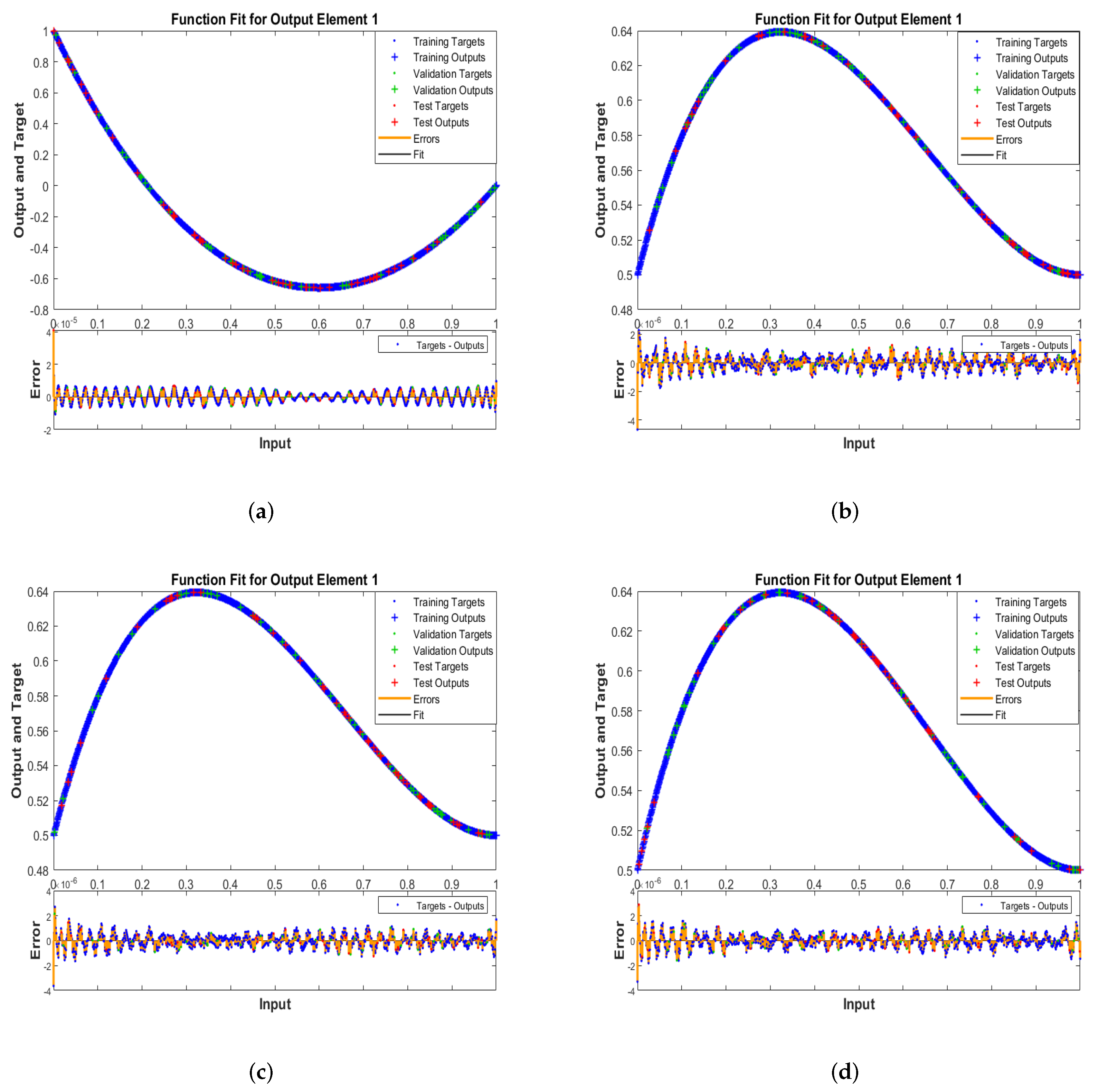
• The processes of training, testing, and validation that are created with (LMB-NN) is implemented for every scenario and case of (MHDSF) to find the approximate solution and comparison with standard results.
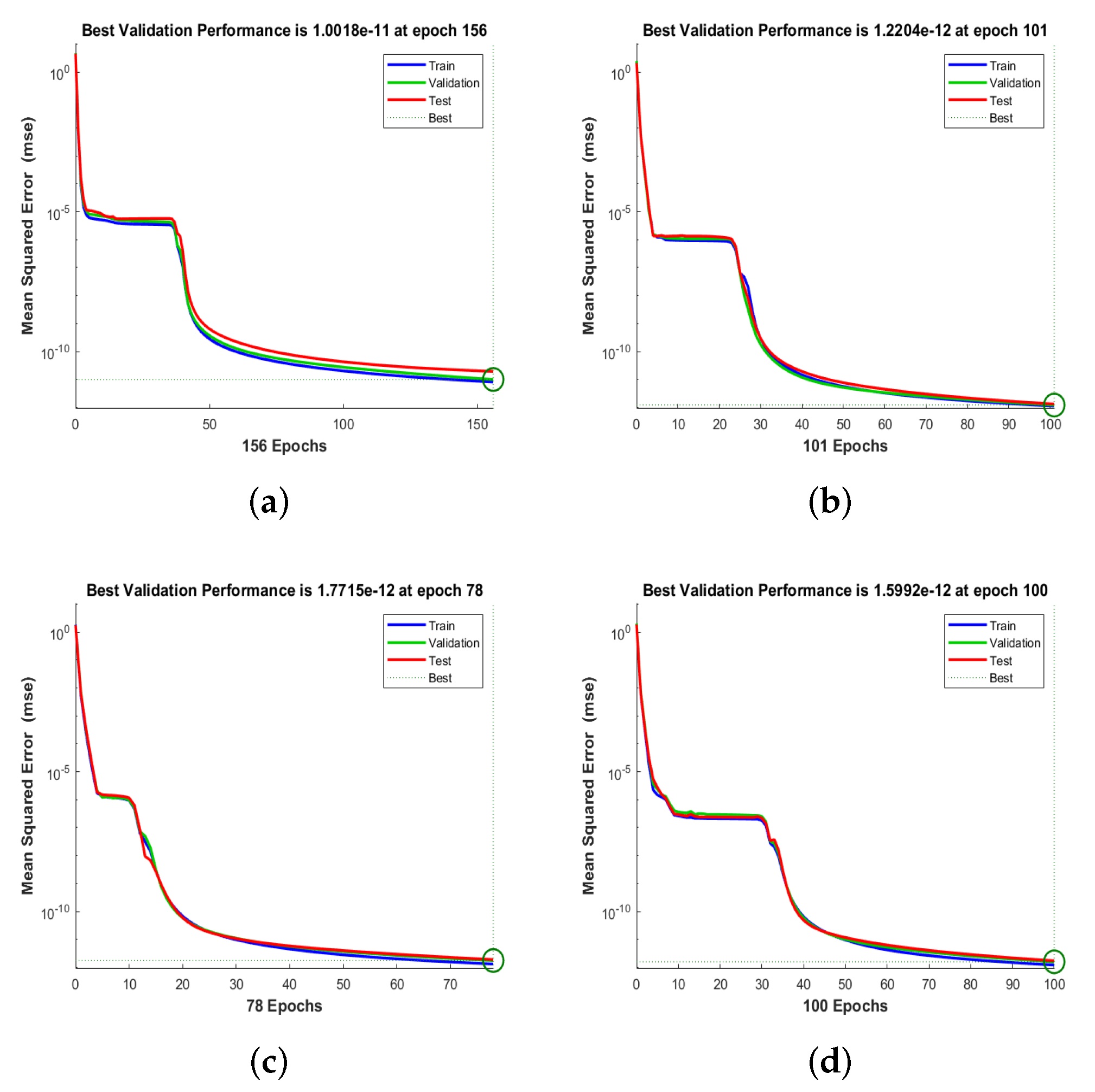
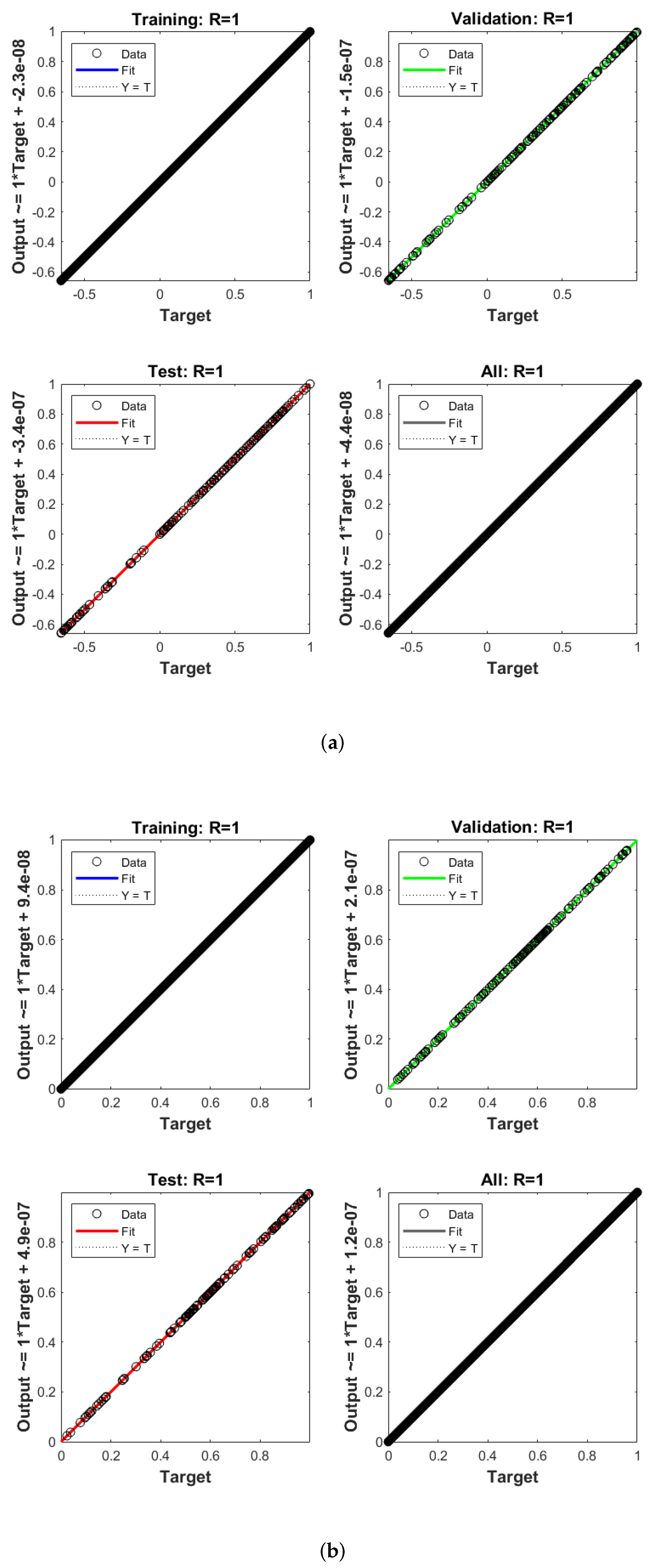
• The performance of NN-BLMS is established through convergence plots of mean squared error-based fitness/merit function, state transition, regression metrics, and histogram error.

The plan for the rest of the paper is as follows: The problem formulation of (MHDSF) is explored in Section 2. The Levenberg–Marquardt algorithm to obtain the solution to the problem is discussed in Section 3. The numerical and graphical results are provided in Section 4. Conclusions are provided in the last section.

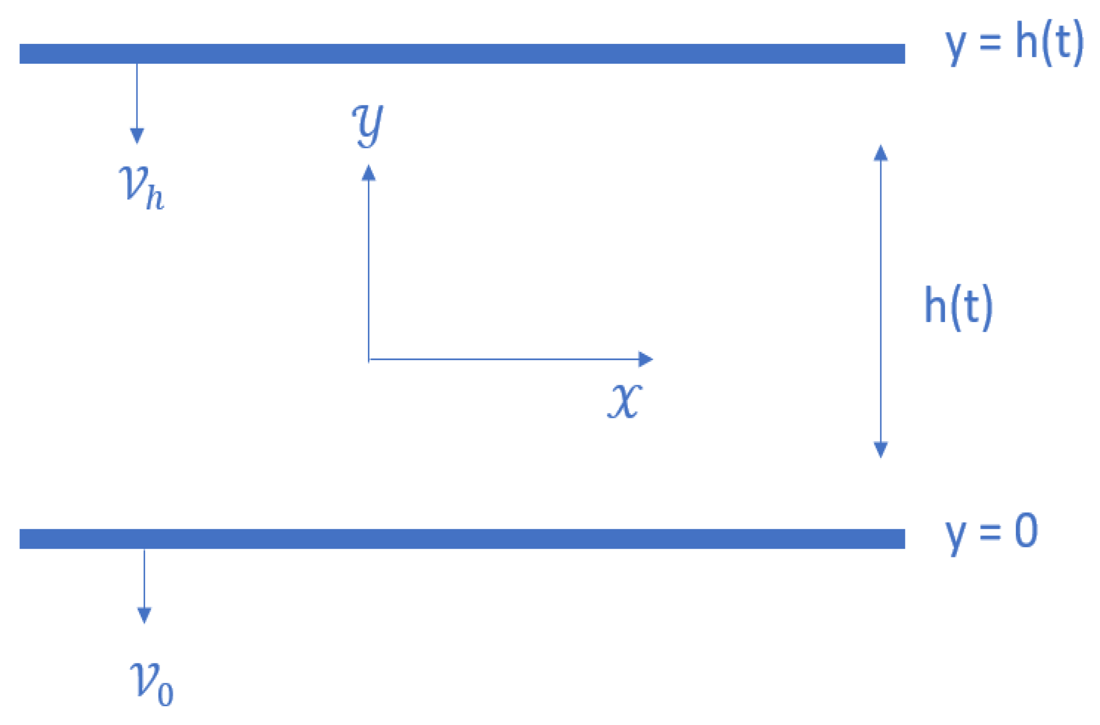
2. Mathematical Formulation

We consider the unsteady squeezing flow of an incompressible two-dimensional viscous nanofluid between two infinite parallel disks Figure 1. The upper disk at $y=h\left(t\right)={\left(\frac{\nu (1-\gamma t)}{a}\right)}^{\frac{1}{2}}$ moves toward the lower stationary disk at $y=0$ with velocity $v_h=\frac{dh}{dt}$. Stretching velocity to the lower disk is $\frac{ax}{(1-\gamma t)}$ and, for $\gamma =0$, the linearly stretching procedure approaches stability in the presence of a magnetic field. Moreover, the effects of thermophoresis and Brownian motion are preserved while neglecting the electric field and Hall effects.

The governing of mass, momentum, energy, and nanoparticle concentration partial differential equations are given as follows [34]:

$$\frac{\partial u}{\partial x}+\frac{\partial v}{\partial y}=0,$$

(1)

$$\frac{\partial u}{\partial t}+u\frac{\partial u}{\partial x}+v\frac{\partial u}{\partial y}=-\frac{1}{{\rho }_f}\frac{\partial p^{*}}{\partial x}+\nu \left(\frac{{\partial }^{2}u}{\partial x^2}+\frac{{\partial }^{2}u}{\partial y^2}\right)-\frac{\sigma B_0^2}{{\rho }_f(1-\gamma t)}u,$$

(2)

$$\frac{\partial v}{\partial t}+u\frac{\partial v}{\partial x}+v\frac{\partial v}{\partial y}=-\frac{1}{{\rho }_f}\frac{\partial p^{*}}{\partial x}+\nu \left(\frac{{\partial }^{2}v}{\partial x^2}+\frac{{\partial }^{2}v}{\partial y^2}\right),$$

(3)

$$\begin{array}{c}\hfill \frac{\partial T}{\partial t}+u\frac{\partial T}{\partial x}+v\frac{\partial T}{\partial y}=\alpha \left(\frac{{\partial }^{2}T}{\partial x^2}+\frac{{\partial }^{2}T}{\partial y^2}\right)+\frac{{\left(\rho c\right)}_p}{{\left(\rho c\right)}_f}{D}_b\left(\frac{\partial T}{\partial x}\frac{\partial C}{\partial x}+\frac{\partial T}{\partial y}\frac{\partial C}{\partial y}\right)\\ \hfill +\frac{{\left(\rho c\right)}_p}{{\left(\rho c\right)}_f}\frac{D_t}{T_M}\left({\left(\frac{\partial T}{\partial x}\right)}^2+{\left(\frac{\partial T}{\partial y}\right)}^2\right),\end{array}$$

(4)

$$\frac{\partial C}{\partial t}+u\frac{\partial C}{\partial x}+v\frac{\partial C}{\partial y}=D_b\left(\frac{{\partial }^{2}C}{\partial x^2}+\frac{{\partial }^{2}C}{\partial y^2}\right)+\frac{D_t}{T_M}\left(\frac{{\partial }^{2}T}{\partial x^2}+\frac{{\partial }^{2}T}{\partial y^2}\right),$$

(5)

subject to the boundary conditions

$$\begin{array}{cc}\hfill u& =U_0=\frac{ax}{1-\gamma t},v=\frac{V_0}{1-\gamma t},T=T_0,C=C_{0}aty=0,\hfill \\ \hfill u& =0,v=v_h=\frac{dh}{dt}=-\frac{\gamma }{2}{\left(\frac{\nu }{a(1-\gamma t)}\right)}^{\frac{1}{2}},T=T_0+\left(\frac{T_0}{(1-\gamma t)}\right),\hfill \\ \hfill C& =C_0+\left(\frac{C_0}{(1-\gamma t)}\right),aty=h\left(t\right).\hfill \end{array}$$

(6)

where $V_0>0$ represents the suction, and $V_0<0$ is the injection/blowing velocity. By using the similarity transformation, the above system yields

$$f^{\prime \prime \prime \prime }+f{f}^{\prime \prime \prime }-f^{\prime }{f}^{\prime \prime }-\frac{\mathrm{Sq}}{2}(3f^{\prime \prime }+\eta f^{\prime \prime \prime })-M^2{f}^{\prime \prime }=0,$$

(7)

$${\theta }^{\prime \prime }+\mathrm{PR}\left(f{\theta }^{\prime }-\frac{\mathrm{Sq}}{2}(2\theta +\eta {\theta }^{\prime })+\mathrm{Nb}{\theta }^{\prime }{\varphi }^{\prime }+\mathrm{Nt}{{\theta }^{\prime }}^2\right)=0,$$

(8)

$${\varphi }^{\prime \prime }+\mathrm{Le} \mathrm{PR}\left(f{\varphi }^{\prime }-\frac{\mathrm{Sq}}{2}(2\varphi +\eta {\varphi }^{\prime })\right)+\frac{\mathrm{Nt}}{\mathrm{Nb}}{\theta }^{\prime \prime }=0,$$

(9)

with the following boundary conditions:

$$\begin{array}{cc}\hfill f\left(0\right)& =\mathrm{S},f^{\prime }\left(0\right)=1,\theta \left(0\right)=0,\varphi \left(0\right)=0,\hfill \\ \hfill f\left(1\right)& =\frac{\mathrm{Sq}}{2},f^{\prime }\left(1\right)=0,\theta \left(1\right)=1,\varphi \left(1\right)=1.\hfill \end{array}$$

(10)

These parameters are defined by

$$\begin{array}{c}\hfill \mathrm{Sq}=\frac{\gamma }{a},M^2=\frac{\sigma B_0^2}{{\rho }_{f}a},\mathrm{S}=\frac{v_0}{ah\left(t\right)},\mathrm{PR}=\frac{\nu }{\alpha },\mathrm{Le}=\frac{\alpha }{D_b},\\ \hfill \mathrm{Nb}=\frac{{\left(\rho c\right)}_p{D}_b{C}_0}{{\left(\rho C\right)}_f\nu (1-\gamma t)},\mathrm{Nt}=\frac{{\left(\rho c\right)}_p{D}_t{T}_0}{{\left(\rho C\right)}_f\nu T_M(1-\gamma t)}\end{array}$$

(11)

3. Solution Methodology

The Levenberg–Marquardt neural network is an algorithm used in nonlinear training. It is proposed for improving the learning algorithm in each of the conjugate gradient and Quasi-Newton methods, where it designs to verify the locally fast convergence speed and achieve better performance in general. The architecture of LMB-NN is shown in Figure 2.

The necessary description of methodology based on neural networks, including the layer structure, hidden neurons, topology of the networks, and arbitrary selection of an input and target data set for training, testing, and validation samples, is determined to solve the problem. With the help of using the “nftoo” command in the neural network toolbox, the suggested LMB-NN is implemented in the MATLAB environment. The total amount of data for LMB-NN is 1001 found between 0 and 1 by setting 0.001 as the stepsize and using the Runge–Kutta technique through “NDSolve” in Mathematica.

These data are distributed randomly for f, $f^{\prime }$, $\theta$, and $\varphi$ into sets: training, testing, and validation to achieve the best convergence. In this problem, we chose the sets as follows:

• $90\%$ of the data for the training.
• $5\%$ of the data for the testing.
• $5\%$ of the data for the validation.

The number of neurons is also arbitrary; selecting 40 gives a good accuracy of the computational results as shown in Figure 3.

4. Results and Discussion

The system of ordinary differential equations of magnetohydrodynamic nanofluid between two parallel plates Equations (7)–(10) is offered here for numerical experimentation of LMB-NN for each case of all scenarios. The scheme of working the LMB-NN is offered in Figure 4. The impact of the variation of different scenarios and cases is listed in

Table 1. Variation of different scenarios and cases involved.

Scenario		Case		Physical Quantities of Interest
				S		M		$\mathit{Nb}$		$\mathit{Nt}$		$\mathit{Sq}$		$\mathit{Le}$		$\mathit{PR}$
(1) Variation in $Sq$		1		0.5		0.5		0.5		0.2		0.0		1.0		1.0
		2		0.5		0.5		0.5		0.2		0.5		1.0		1.0
		3		0.5		0.5		0.5		0.2		1.0		1.0		1.0
		4		0.5		0.5		0.5		0.2		1.5		1.0		1.0
(2) Variation in $PR$		1		0.5		0.5		0.5		0.2		1.0		1.0		0.5
		2		0.5		0.5		0.5		0.2		1.0		1.0		1.0
		3		0.5		0.5		0.5		0.2		1.0		1.0		1.5
		4		0.5		0.5		0.5		0.2		1.0		1.0		2.0
(3) Variation in $Nb$		1		0.5		0.5		0.5		0.2		1.0		1.0		1.0
		2		0.5		0.5		1.0		0.2		1.0		1.0		1.0
		3		0.5		0.5		1.5		0.2		1.0		1.0		1.0
		4		0.5		0.5		2.0		0.2		1.0		1.0		1.0
(4) Variation in $Nt$		1		0.5		0.5		0.5		0.0		1.0		1.0		1.0
		2		0.5		0.5		0.5		0.3		1.0		1.0		1.0
		3		0.5		0.5		0.5		0.6		1.0		1.0		1.0
		4		0.5		0.5		0.5		1.0		1.0		1.0		1.0

. The graphs and tables below present the numerical results of some exciting parameters on interest profiles.

Figure 5 explains the performance interpretation of AI computing concerning main square error (MSE) for case 2 of scenarios 1, 2, 3, and 4, respectively. The minimum value of (MSE) reached in scenario 2 is estimated by ($1.2204\times {10}^{-12}$) at (101) epochs. This means that it obtained the best accuracy of the (LMB-NN) compared to the other scenarios. The fitness plots along with error dynamics for input between 0 to 1 and step size $0.001$ are shown in Figure 6 for case 2 of all scenarios performed to solve (MHDSF) with LMB-NN.

The training states of the gradient, Mu, and validation checks are shown in Figure 7 for case 2 of scenarios 1, 2, 3, and 4, respectively. The gradient updates the weights of the neural network in the correct direction and amount, while Mu is the value used to control the training algorithm, and the validation check is expressed as the generalization standard of the system. The difference between targets and output values appears in Figure 8, where the zero error line indicates the smallest distance present in the error histogram. Comparing all the values referred to in Case 2 from all four scenarios shows that the smallest value was executed at $-2.2\times {10}^{-8}$, therefore achieving the proposed model’s best accuracy. The regression studies are presented in Figure 9 and Figure 10 for all training, testing, and validation that is used to solve (MHDSF), and the value of R is equal to one for different scenarios. Thus, the target accuracy of the proposed model has been accomplished. Therefore, the results obtained from running in LMB-NN are displayed for velocity, temperature, and concentration profiles, respectively, for different scenarios (MHDSF) close to the results we found from the Runge–Kutta method, as seen in Figure 11. The absolute error (AE) is computing to establish an accurate benchmark for comparison; Figure 12 offered the (AE) from the reference solution for all scenarios, and the smallest (AE) is shown in scenario 4. Organize the computational operations include MSE processes, performance, gradient, Mu, epoch, and time in

Table 2. NN-BLMS numerical outcomes for the MHDSF system.

Scenarios (S)	Case	Main Square Error			Performance	Gradient	Mu Value	Epochs	Time
		Training	Validation	Testing
(1)	1	4.76585 $\times {10}^{-12}$	6.30371 $\times {10}^{-12}$	6.3129$\times {10}^{-12}$	4.77$\times {10}^{-12}$	9.94$\times {10}^{-8}$	1.00$\times {10}^{-12}$	256	≤0.5
	2	8.13009$\times {10}^{-12}$	1.00178$\times {10}^{-11}$	1.95386$\times {10}^{-11}$	8.13$\times {10}^{-12}$	9.87$\times {10}^{-8}$	1.00$\times {10}^{-12}$	156	≤0.5
	3	4.31321$\times {10}^{-6}$	3.26626$\times {10}^{-6}$	5.19729$\times {10}^{-6}$	3.24$\times {10}^{-6}$	3.14$\times {10}^{-5}$	1.00$\times {10}^{-7}$	135	≤0.5
	4	1.21850$\times {10}^{-11}$	1.54756$\times {10}^{-11}$	1.42292$\times {10}^{-11}$	1.22$\times {10}^{-11}$	9.80$\times {10}^{-8}$	1.00$\times {10}^{-12}$	123	≤0.5
(2)	1	7.63307$\times {10}^{-7}$	1.09583$\times {10}^{-6}$	1.02174$\times {10}^{-6}$	7.33$\times {10}^{-7}$	1.16$\times {10}^{-6}$	1.00$\times {10}^{-8}$	17	≤0.5
	2	1.12830$\times {10}^{-12}$	1.22042$\times {10}^{-12}$	1.32671$\times {10}^{-12}$	1.13$\times {10}^{-12}$	9.87$\times {10}^{-8}$	1.00$\times {10}^{-13}$	101	≤0.5
	3	1.26984$\times {10}^{-12}$	1.82527$\times {10}^{-12}$	1.74307$\times {10}^{-12}$	1.27$\times {10}^{-12}$	9.74$\times {10}^{-8}$	1.00$\times {10}^{-13}$	94	≤0.5
	4	1.29840$\times {10}^{-12}$	1.77428$\times {10}^{-12}$	1.72913$\times {10}^{-12}$	1.30$\times {10}^{-12}$	9.97$\times {10}^{-8}$	1.00$\times {10}^{-13}$	80	≤0.5
(3)	1	1.25823$\times {10}^{-12}$	1.94858$\times {10}^{-12}$	1.80848$\times {10}^{-12}$	1.26$\times {10}^{-12}$	9.79$\times {10}^{-8}$	1.00$\times {10}^{-13}$	86	≤0.5
	2	1.33239$\times {10}^{-12}$	1.77148$\times {10}^{-12}$	1.91072$\times {10}^{-12}$	1.33$\times {10}^{-12}$	9.95$\times {10}^{-8}$	1.00$\times {10}^{-13}$	78	≤0.5
	3	1.20463$\times {10}^{-12}$	1.54025$\times {10}^{-12}$	1.25176$\times {10}^{-12}$	1.20$\times {10}^{-12}$	9.99$\times {10}^{-8}$	1.00$\times {10}^{-13}$	98	≤0.5
	4	1.18896$\times {10}^{-6}$	1.60196$\times {10}^{-6}$	1.70214$\times {10}^{-6}$	1.11$\times {10}^{-6}$	2.43$\times {10}^{-6}$	1.00$\times {10}^{-8}$	16	≤0.5
(4)	1	9.73136$\times {10}^{-7}$	1.02015$\times {10}^{-6}$	1.16425$\times {10}^{-6}$	9.28$\times {10}^{-7}$	1.72$\times {10}^{-6}$	1.00$\times {10}^{-8}$	24	≤0.5
	2	1.22586$\times {10}^{-12}$	1.59916$\times {10}^{-12}$	1.73599$\times {10}^{-12}$	1.23$\times {10}^{-12}$	9.80$\times {10}^{-8}$	1.00$\times {10}^{-13}$	100	≤0.5
	3	1.11988$\times {10}^{-12}$	1.47276$\times {10}^{-12}$	1.21307$\times {10}^{-12}$	1.12$\times {10}^{-12}$	9.96$\times {10}^{-8}$	1.00$\times {10}^{-13}$	113	≤0.5
	4	1.45146$\times {10}^{-6}$	1.64029$\times {10}^{-6}$	1.58078$\times {10}^{-6}$	1.41$\times {10}^{-6}$	6.48$\times {10}^{-6}$	1.00$\times {10}^{-8}$	16	≤0.5

.

5. Conclusions

Modern artificial intelligence computing is developed to obtain numerical results for the governing mathematical formulation (MHDSF) analysis using the Levenberg–Marquardt backpropagated algorithm. These results are compared with standard solutions that come with the help of the explicit Runge–Kutta method. The best compatibility is achieved around ${10}^{-6}$ to ${10}^{-3}$, which means that the consistent accuracy of the (LMB-NN) is investigated. Notice that the velocity profile increases with the squeezing parameter $Sq$, while the temperature profile is enhanced with higher Prandtl number PR values. Otherwise, the increase of the parameter of Brownian motion $Nb$ enhanced the temperature profile; in addition, the concentration profile decreases when the thermophoresis parameter values are $Nt$ increasing. New AI algorithms will be improved to obtain more accurate results in the future [35,36].

References

1. Stefan, J. Versuche über die scheinbare Adhäsion. Ann. Der Phys. 1875, 230, 316–318. [Google Scholar] [CrossRef] [Green Version]
2. Reynolds, O. IV. On the theory of lubrication and its application to Mr. Beauchamp tower’s experiments, including an experimental determination of the viscosity of olive oil. Philos. Trans. R. Soc. Lond. 1886, 177, 157–234. [Google Scholar]
3. Atlas, M.; Haq, R.U.; Mekkaoui, T. Active and zero flux of nanoparticles between a squeezing channel with thermal radiation effects. J. Mol. Liq. 2016, 223, 289–298. [Google Scholar] [CrossRef]
4. Domairry, G.; Hatami, M. Squeezing Cu–water nanofluid flow analysis between parallel plates by DTM-Padé Method. J. Mol. Liq. 2014, 193, 37–44. [Google Scholar] [CrossRef]
5. Domairry, G.; Aziz, A. Approximate analysis of MHD squeeze flow between two parallel disks with suction or injection by homotopy perturbation method. Math. Probl. Eng. 2009, 2009, 603916. [Google Scholar] [CrossRef] [Green Version]
6. Buongiorno, J. Convective transport in nanofluids. J. Heat Transf. 2006, 128, 240–250. [Google Scholar] [CrossRef]
7. Khan, W.A.; Pop, I. Boundary-layer flow of a nanofluid past a stretching sheet. Int. J. Heat Mass Transf. 2010, 53, 2477–2483. [Google Scholar] [CrossRef]
8. Turkyilmazoglu, M. Exact analytical solutions for heat and mass transfer of MHD slip flow in nanofluids. Chem. Eng. Sci. 2012, 84, 182–187. [Google Scholar] [CrossRef]
9. Masuda, H.; Ebata, A.; Teramae, K. Alteration of thermal conductivity and viscosity of liquid by dispersing ultra-fine particles. Dispersion of Al2O3, SiO2 and TiO2 ultra-fine particles. NETSU BUSSEI 1993, 7, 227–233. [Google Scholar] [CrossRef]
10. CChoi, S.U.S.; Eastman, J.A. Enhancing Thermal Conductivity of Fluids with Nanoparticles; No. ANL/MSD/CP-84938; CONF-951135-29; Argonne National Lab.: Lemont, IL, USA, 1995. [Google Scholar]
11. Eastman, J.A.; Choi, S.U.S.; Li, S.; Yu, W.; Thompson, L.J. Anomalously increased effective thermal conductivities of ethylene glycol-based nanofluids containing copper nanoparticles. Appl. Phys. Lett. 2001, 78, 718–720. [Google Scholar] [CrossRef]
12. Shoaib, M.; Raja, M.A.Z.; Sabir, M.T.; Awais, M.; Islam, S.; Shah, Z.; Kumam, P. Numerical analysis of 3D MHD hybrid nanofluid over a rotational disk in the presence of thermal radiation with Joule heating and viscous dissipation effects using Lobatto IIIA technique. Alex. Eng. J. 2021, 60, 3605–3619. [Google Scholar] [CrossRef]
13. Nagoor, A.H.; Alaidarous, E.S.; Sabir, M.T.; Shoaib, M.; Raja, M.A.Z. Numerical treatment for three-dimensional rotating flow of carbon nanotubes with Darcy–Forchheimer medium by the Lobatto IIIA technique. Aip Adv. 2020, 10, 025016. [Google Scholar] [CrossRef] [Green Version]
14. Shoaib, M.; Raja, M.A.Z.; Sabir, M.T.; Islam, S.; Shah, Z.; Kumam, P.; Alrabaiah, H. Numerical investigation for rotating flow of MHD hybrid nanofluid with thermal radiation over a stretching sheet. Sci. Rep. 2020, 10, 1–15. [Google Scholar] [CrossRef]
15. Bukhari, A.H.; Sulaiman, M.; Raja, M.A.Z.; Islam, S.; Shoaib, M.; Kumam, P. Design of a hybrid NAR-RBFs neural network for nonlinear dusty plasma system. Alex. Eng. J. 2020, 59, 3325–3345. [Google Scholar] [CrossRef]
16. Bukhari, A.H.; Raja, M.A.Z.; Sulaiman, M.; Islam, S.; Shoaib, M.; Kumam, P. Fractional neuro-sequential ARFIMA-LSTM for financial market forecasting. IEEE Access 2020, 8, 71326–71338. [Google Scholar] [CrossRef]
17. Bukhari, A.H.; Sulaiman, M.; Islam, S.; Shoaib, M.; Kumam, P.; Raja, M.A.Z. Neuro-fuzzy modeling and prediction of summer precipitation with application to different meteorological stations. Alex. Eng. J. 2020, 59, 101–116. [Google Scholar] [CrossRef]
18. Ahmad, I.; Ilyas, H.; Urooj, A.; Aslam, M.S.; Shoaib, M.; Raja, M.A.Z. Novel applications of intelligent computing paradigms for the analysis of nonlinear reactive transport model of the fluid in soft tissues and microvessels. Neural Comput. Appl. 2019, 31, 9041–9059. [Google Scholar] [CrossRef]
19. Waseem, W.; Sulaiman, M.; Kumam, P.; Shoaib, M.; Raja, M.A.Z.; Islam, S. Investigation of singular ordinary differential equations by a neuroevolutionary approach. PLoS ONE 2020, 15, e0235829. [Google Scholar] [CrossRef] [PubMed]
20. Waseem, W.; Sulaiman, M.; Islam, S.; Kumam, P.; Nawaz, R.; Raja, M.A.Z.; Farooq, M.; Shoaib, M. A study of changes in temperature profile of porous fin model using cuckoo search algorithm. Alex. Eng. J. 2020, 59, 11–24. [Google Scholar] [CrossRef]
21. Ilyas, H.; Ahmad, I.; Raja, M.A.Z.; Shoaib, M. A novel design of Gaussian WaveNets for rotational hybrid nanofluidic flow over a stretching sheet involving thermal radiation. Int. Commun. Heat Mass Transf. 2021, 123, 105196. [Google Scholar] [CrossRef]
22. Khan, I.; Raja, M.A.Z.; Shoaib, M.; Kumam, P.; Alrabaiah, H.; Shah, Z.; Islam, S. Design of Neural Network With Levenberg–Marquardtt and Bayesian Regularization Backpropagation for Solving Pantograph Delay Differential Equations. IEEE Access 2020, 8, 137918–137933. [Google Scholar] [CrossRef]
23. Sabir, Z.; Umar, M.; Guirao, J.L.; Shoaib, M.; Raja, M.A.Z. Integrated intelligent computing paradigm for nonlinear multi-singular third-order Emden–Fowler equation. Neural Comput. Appl. 2020, 33, 1–20. [Google Scholar] [CrossRef]
24. Sabir, Z.; Raja, M.A.Z.; Umar, M.; Shoaib, M. Design of neuro-swarming-based heuristics to solve the third-order nonlinear multi-singular Emden–Fowler equation. Eur. Phys. J. Plus 2020, 135, 1–17. [Google Scholar] [CrossRef]
25. Sabir, Z.; Raja, M.A.Z.; Guirao, J.L.; Shoaib, M. Integrated intelligent computing with neuro-swarming solver for multi-singular fourth-order nonlinear Emden–Fowler equation. Comput. Appl. Math. 2020, 39, 1–18. [Google Scholar] [CrossRef]
26. Umar, M.; Sabir, Z.; Raja, M.A.Z.; Aguilar, J.G.; Amin, F.; Shoaib, M. Neuro-swarm intelligent computing paradigm for nonlinear HIV infection model with CD4+ T-cells. Math. Comput. Simul. 2021, 188, 241–253. [Google Scholar] [CrossRef]
27. Shoaib, M.; Raja, M.A.Z.; Sabir, M.T.; Bukhari, A.H.; Alrabaiah, H.; Shah, Z.; Kumam, P.; Islam, S. A Stochastic Numerical Analysis Based on Hybrid NAR-RBFs Networks Nonlinear SITR Model for Novel COVID-19 Dynamics. Comput. Methods Programs Biomed. 2021, 202, 105973. [Google Scholar] [CrossRef]
28. Ahmad, I.; Raja, M.A.Z.; Ramos, H.; Bilal, M.; Shoaib, M. Integrated neuro-evolution-based computing solver for dynamics of nonlinear corneal shape model numerically. Neural Comput. Appl. 2020, 33, 5753–5769. [Google Scholar] [CrossRef]
29. Umar, M.; Raja, M.A.Z.; Sabir, Z.; Alwabli, A.S.; Shoaib, M. A stochastic computational intelligent solver for numerical treatment of mosquito dispersal model in a heterogeneous environment. Eur. Phys. J. Plus 2020, 135, 1–23. [Google Scholar] [CrossRef]
30. Faisal, F.; Shoaib, M.; Raja, M.A.Z. A new heuristic computational solver for nonlinear singular Thomas–Fermi system using evolutionary optimized cubic splines. Eur. Phys. J. Plus 2020, 135, 1–29. [Google Scholar]
31. Uddin, I.; Ullah, I.; Raja, M.A.Z.; Shoaib, M.; Islam, S.; Muhammad, T. Design of intelligent computing networks for numerical treatment of thin film flow of Maxwell nanofluid over a stretched and rotating surface. Surf. Interfaces 2021, 24, 101107. [Google Scholar] [CrossRef]
32. Shoaib, M.; Raja, M.A.Z.; Khan, M.A.R.; Farhat, I.; Awan, S.E. Neuro-Computing Networks for Entropy Generation under the Influence of MHD and Thermal Radiation. Surf. Interfaces 2021, 25, 101243. [Google Scholar] [CrossRef]
33. Aljohani, J.L.; Alaidarous, E.S.; Raja, M.A.Z.; Shoaib, M.; Alhothuali, M.S. Intelligent computing through neural networks for numerical treatment of non-Newtonian wire coating analysis model. Sci. Rep. 2021, 11, 1–32. [Google Scholar] [CrossRef] [PubMed]
34. Hayat, T.; Muhammad, T.; Qayyum, A.; Alsaedi, A.; Mustafa, M. On squeezing flow of nanofluid in the presence of magnetic field effects. J. Mol. Liq. 2016, 213, 179–185. [Google Scholar] [CrossRef]
35. Shoaib, M.; Akhtar, R.; Khan, M.A.R.; Rana, M.A.; Siddiqui, A.M.; Zhiyu, Z.; Raja, M.A.Z. A Novel Design of Three-Dimensional MHD Flow of Second-Grade Fluid past a Porous Plate. Math. Probl. Eng. 2019, 2019, 584397. [Google Scholar] [CrossRef] [Green Version]
36. Imran, A.; Akhtar, R.; Zhiyu, Z.; Shoaib, M.; Zahoor Raja, M.A. MHD and heat transfer analyses of a fluid flow through scraped surface heat exchanger by analytical solver. Aip Adv. 2019, 9, 075201. [Google Scholar] [CrossRef] [Green Version]
Figure 1. Configuration of the system.
Coatings 11 00779 g001
Figure 2. Design of a single neural network.
Coatings 11 00779 g002
Figure 3. Model generated using the NN toolbox.
Coatings 11 00779 g003
Figure 4. Work flow diagram of proposed LMB-NN for the (MHDSF) model.
Coatings 11 00779 g004
Figure 5. MSE performance of the LMB-NN paradigm for (MHDSF). (a) MSE curve for (case 2-S1); (b) MSE curve for (case 2-S2); (c) MSE curve for (case 2-S3); (d) MSE curve for (case 2-S4).
Coatings 11 00779 g005
Figure 6. Assessment of the LMB-NN paradigm for (MHDSF). (a) Fitness outline for (case 2-S1); (b) Fitness outline for (case 2-S2); (c) Fitness outline for (case 2-S3); (d) Fitness outline for (case 2-S4).
Coatings 11 00779 g006
Figure 7. State transition of the LMB-NN paradigm for (MHDSF). (a) State outcomes for (case 2-S1); (b) State outcomes for (case 2-S2); (c) State outcomes for (case 2-S3); (d) State outcomes for (case 2-S4).
Coatings 11 00779 g007
Figure 8. The error of the histogram of the LMB-NN paradigm for (MHDSF). (a) The error of histogram for (case 2-S1); (b) The error of histogram for (case 2-S2); (c) The error of histogram for (case 2-S3); (d) The error of histogram for (case 2-S4).
Coatings 11 00779 g008
Figure 9. Regression views of the LMB-NN paradigm for (MHDSF) for (S1–S2). (a) Regression presentation for (case 2-S1) and (b) Regression presentation for (case 2-S2).
Coatings 11 00779 g009
Figure 10. Regression views of the LMB-NN paradigm for (MHDSF) for (S3–S4). (a) Regression presentation for (case 2-S3) and (b) Regression presentation for (case 2-S4).
Coatings 11 00779 g010
Figure 11. Comparison of obtained results through LMB-NN for case 2 for the (MHDSF) model. (a) Variation of S q ; (b) Variation of P R ; (c) Variation of N b ; (d) Variation of N t .
Coatings 11 00779 g011
Figure 12. The absolute error of case 2 for all scenarios of the (MHDSF) model. (a) Analysis on AE of S1; (b) Analysis on AE of S2 (c); Analysis on AE of S3; (d) Analysis on AE of S4.
Coatings 11 00779 g012