Article

Thermal Analysis and Optimization of Nano Coated Radiator Tubes Using Computational Fluid Dynamics and Taguchi Method

by
Sudalai Suresh Pungaiah
1,* and
Chidambara Kuttalam Kailasanathan
2
1
Department of Mechanical Engineering, SRM Valliammai Engineering College, Chennai 603203, Tamil Nadu, India
2
Department of Mechanical Engineering, Sethu Institute of Technology, Virudhunagar 626115, Tamil Nadu, India
*
Author to whom correspondence should be addressed.
Coatings 2020, 10(9), 804; https://doi.org/10.3390/coatings10090804
Submission received: 27 June 2020 / Revised: 10 August 2020 / Accepted: 15 August 2020 / Published: 20 August 2020
(This article belongs to the Section Liquid–Fluid Coatings, Surfaces and Interfaces)

Abstract

:
Automotive heat removal levels are of high importance for maximizing fuel consumption. Current radiator designs are constrained by air-side impedance, and a large front field must meet the cooling requirements. The enormous demand for powerful engines in smaller hood areas has caused a lack of heat dissipation in the vehicle radiators. As a prediction, exceptional radiators are modest enough to understand coolness and demonstrate great sensitivity to cooling capacity. The working parameters of the nano-coated tubes are studied using Computational Fluid Dynamics (CFD) and Taguchi methods in this article. The CFD and Taguchi methods are used for the design of experiments to analyse the impact of nano-coated radiator parameters and the parameters having a significant impact on the efficiency of the radiator. The CFD and Taguchi methodology studies show that all of the above-mentioned parameters contribute equally to the rate of heat transfer, effectiveness, and overall heat transfer coefficient of the nanocoated radiator tubes. Experimental findings are examined to assess the adequacy of the proposed method. In this study, the coolant fluid was transmitted at three different mass flow rates, at three different coating thicknesses, and coated on the top surface of the radiator tubes. Thermal analysis is performed for three temperatures as heat input conditioning for CFD. The most important parameter for nanocoated radiator tubes is the orthogonal array, followed by the Signal-to-Noise Ratio (SNRA) and the variance analysis (ANOVA). A proper orthogonal array is then selected and tests are carried out. The findings of ANOVA showed 95% confidence and were confirmed in the most significant parameters. The optimal values of the parameters are obtained with the help of the graphs.

1. Introduction

Surface engineering involves the development of a wide range of technologies for component surface characteristics and adaptation. Surface modifications may be used to reduce friction, increase surface wear, increase resistance to corrosion, increase heat transfer, and alter the physical or mechanical properties of the component [1]. Surface additives may also be paired with surface coating methods, such as laser coating, physical vapor deposition (PVD), chemical vapor deposition (CVD), a thermal spraying method, sol-gel, coating and galvanizing. This blend improves the benefits of surface coating and surface modification to meet individual safety and needs. The automotive radiator is a key component of the engine cooling system. The problem of inadequate dissipation rates in automotive radiators has been caused by the demand for more powerful vehicles in smaller hoods. Moreover, a large number of heaters should be redesigned to become lighter while still having sufficient cooling capabilities [2].
Engine oils and lubricants decompose at temperatures above the optimum range and induce expansion in moving parts. Engines are assembled to fit tightly, which leads to dangerous metal contact due to the marginal expansion of the parts [3]. Likewise, an overcooled engine can be exposed to high thermal stress and a loss of material strength (i.e., below optimal temperature). This is because the temperature is monitored using a thermostat in most radiator cooling systems [4]. This thermostat will remain closed until the temperature of the coolant reaches a certain point, under which the coolant is maintained within the engine [5,6].
Today’s engine requires higher efficiency with less space available to allow for the flow of coolant. This requires a better knowledge of the complex refractive fluid stream characteristics and heat quality of the heat sink [7].
Normally, the heat transfer from surfaces can be increased by increasing the coefficient of heat transfer between the surface and its surroundings, by enhancing the surface area of heat transfer, or by both. There are many approaches to improve the characteristics of heat transfer, which can primarily be separated into active and passive techniques [8].
Active techniques are more convenient to use and design components. As the system needs some external power input, it will induce the desired change inflow and increase the rate of heat transfer. It requires limited use due to the need for external control in many functional applications. Increased heat transfer by this process can be accomplished by mechanical use, surface vibration, fluid vibration, electrostatic forces, compression, suction, and jet impingement.
Passive methods typically use surface or geometric modifications to the flow channel by adding extensions or unessential contrivances to promote higher coefficients of heat transfer by disturbing or modifying the subsistent flow attitudes, such as treated surfaces, rough surfaces, elongated surfaces, displacement enhancement contrivances, swirl flow contrivances, coiled tubing, and surface tension contrivances. Passive techniques are more important in these contexts, since active techniques are more complex from a design viewpoint [9,10].
Material coatings are often used for tribological applications to reduce friction, fouling, and wear. Although the make-up of the nano-coating was classified as proprietary in nature in this report, an analysis of the related literature is provided to include contextual details for their intent, intended usage and implementation. Nano-coatings may be broadly described as any substance having at least one component occurring on the nanometer scale where the main component is called the matrix and the fillers are scattered throughout [11].
The evaluated nano-coating technology may also be a solution to increase the effectiveness of thermal exchangers and thus the overall engine performance. Through using a material layer that helps to increase the heat transfer rate or decrease the friction between the fluid flow and the corresponding cooler walls on the current base, the performance of the engine can be improved while decreasing fuel consumption. The use of material coatings on heat exchanger surfaces will reduce some of the implications, resulting in higher heat transfer levels. From a macroscopic perspective, it has been shown that, generally, the engine output is improved considerably when fuel consumption is decreased after cooler operations.

2. Taguchi Method

The experimental design using the Taguchi orthogonal array will full-fill the requirements of problem-solving and product optimization projects economically [12]. By introducing Taguchi methodologies, the time, effort, and money for experimental work can be minimized by researchers, engineers, and scientists. The design of experiments (DOE) defines the relationship between the variable’s input and output. The DOE with Taguchi orthogonal array needs good preparation, intelligent experiment structure, and specialist result interpretation. The Taguchi method became the traditional DOE method [13,14]. It was designed by Dr. Genechi Taguchi (1940 by the Japanese engineer) and came to be known as one of the best plays for scientists and engineers [15].
The DOE’s principal goal is for the input and output parameters to be further and more practical. A large number of experiments are needed for more and more accurate knowledge. However, modern experimental theory indicates that this is not always valid [16]. The full number of experiments is an enormous mistake in terms of cost. It is easier to collect more and more practical data when playing with less [17]. Taguchi’s approach is one of the best examples. Taguchi developed a technique called orthogonal selection to review all process parameters with minimum equilibrium tests only [18]. The primary purpose of the DOE is to analyze the parameter (entry) that affects the performance more effectively. The approach to enhance product quality is well known, strong, and unique [19].
Taguchi is computational techniques for optimizing design, using the traditional “Orthogonal Arrays” to construct an experiment matrix to achieve minimum experimental numbers for the greatest number of data. In Taguchi techniques, the number of parameters can be measured at a time with probably fewer experiments than others. Moreover, the technique contains all the knowledge needed to optimize the problem. The main advantage of Taguchi techniques is not only the smallest number of experiments possible, but the best quantity of each parameter with each parameter divided into the problem [20]. Qualitative features and design criteria for the product/process, experimental design and behavior, results evaluation for optimal specifications, and confirmatory tests to be carried out under optimal conditions are all key steps of the Taguchi process shown in Figure 1.
The better and less all the values observed are calculated by the equation in the Taguchi method. The findings in this analysis include the mean, minimum and average output values, effectiveness and overall coefficient of heat transfer. Parameters for control (Design factors) and their levels are listed in Table 1 and Three level considerations orthogonal array for L9 are listed in Table 2.

3. Analysis of Variance (ANOVA)

The following experimental results were evaluated with variance analyses.
Variance   ( V )   =   Sum   of   Squares Degrees   of   Freedom   =   S T f
ST = nσ2nm2
Sm = σ2nm2
Se = STSm = (n − 1)σ2
Also, as previously mentioned, variance (V) is V = S f . Therefore,
VT = ST/fT = σ2 + m2 (Total Variance)
Vm = Sm/fm = σ2 + nm2 (Mean Variance)
Ve = (STSm)/fe = σ2 (Error Variance)
The sound-to-noise ratio analysis (S/N ratio) has been designed for quality measurement.

4. Result Conversion to S/N Ratios

A collection of measurements, the SNRA, is converted into one single number in two steps. Next, measurement is made of the mean square deviation (MSD) of the package. Third, by definition, the SNRA determined from the MSD,
S/N = −10log10 (MSD)
MSD = (Y12 + Y22 + …YN2)/N
Correction   factor   ( C . F )   =   ( Sum   of   SNRA )   2 N
Sum   of   Squares   =   { ( sum   of   SNRA   1 st   level )   +   ( sum   of   SNRA   2 nd   level )   +   ( sum   of   SNRA   3 rd   level )     C . F } 2
Percentage   of   Contribution   =   Sum   of   Squares   of   a   Parameters Total   Sum   of   Squares
where Yi is the characteristic for output or performance and N is the total number of experiments.

5. Experimental Setup

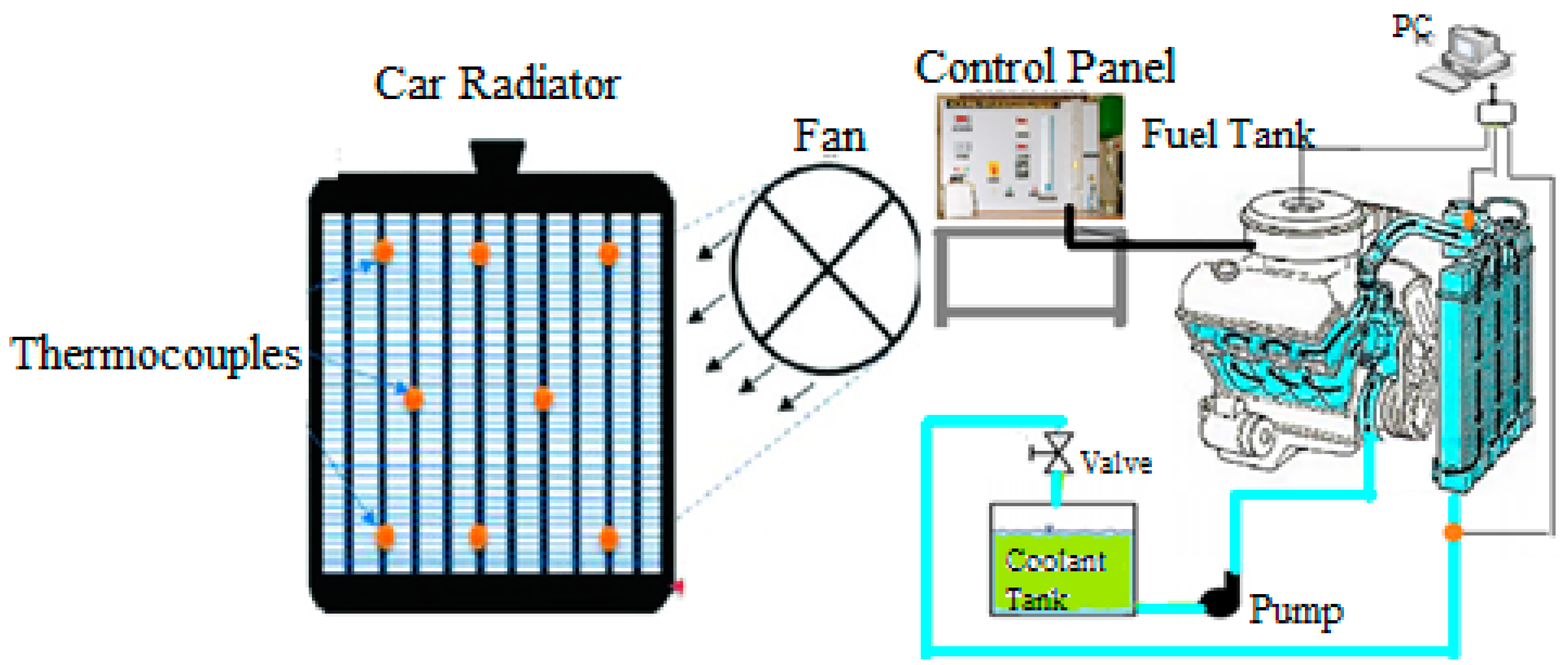
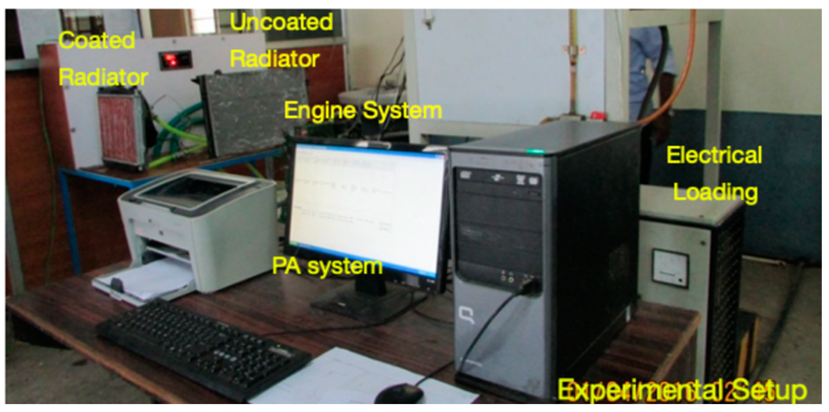
The experimental diagram and setup are shown in Figure 2 and Figure 3. Table 3, displays the design of the radiator and engine set-up of the nano-coated tube radiator. A radiator is one kind of heat exchanger. The intention is to transfer heat from the coolant to the fan’s air.
Instead of formability and costs, most modern cars use aluminium radiators. Copper coated aluminium tubes are used in place of aluminium pipes, and thin aluminium fins are used to make these radiators. The coolant passes through several tubes in parallel from the entrance to the outlet. The fins led the heat through the heat sink, from the tube to the air [21,22].
Copper has a higher thermal conductivity than aluminum to dissipate more heat at a higher rate, thereby increasing the engine power to the next level, and measuring the efficiency of the radiator [23]. Experimental procedures have been replicated for different water mass flow rates and different radiator tube thicknesses have been reported, as well as observations.

6. CFD Model Analysis

In solid work, the three-dimensional model of the radiator was generated and exported to an IGS file as a single layer. The original designs have been modeled as one region, and characteristics not involved in internal flow have been eliminated. ANSYS CFD software was used in meshing and CFD analysis.

7. Geometry

A cuboid, supplied with porous media, was the heart of the radiator. The center of the calculation has dimensions of 500 × 500 × 30 mm3. There is an entrance pipe in the header over the radiator and there was an outlet pipe below the header that guided the water flow. The air regions were represented by the two cuboids in front of and behind the radiator [17,24]. The inlet and outlet for both fluids and interfaces between the various bodies was created before the meshing and selection of the physical model [25]. A new area was established to define different borders.

8. Mesh

The core section of the geometric model was given a finer mesh (Figure 4) than the other geometry regions to reduce the time of the CPU and load on the computer. The basic dimensions for the core section were 0.64 m. The base size was set at 2.56 m for the air region.

9. Physical Models

The physical model for the radiator was chosen to determine the type of flow.
Different models have been developed as two fluids have been studied.
  • Two Layer All and Wall Treatment
  • Realizable K-Epsilon
  • Two Layer Reynolds-Mean
Navier-Stokes Separate Fluid Temperature Air physical model:
Gas Water physical model: Two-dimensional Gradient Steady Stream One Layer Two Layer All and Wall Treated Towers.

10. Boundary Conditions

Coolant InletMass Flow Rate
Coolant OutletPressure Outlet
Air InletVelocity Inlet
Air OutletVelocity Outlet

11. Thermal Simulation

It is required to analyze the thermal performance of a tube composed by aluminium and a coat of copper. The dimensions of the tube are presented in Figure 5, and the physical properties of the materials considered are shown in Table 4. Water enters to the tube at a temperature of 323, 343, and 363 K and with a mass flow rate of 0.15, 0.30, and 0.45 L/min, whilst the tube is exposed to air at 25 °C with a convective heat transfer coefficient of 450 W m−2 K−1. Three different thicknesses will be simulated for the copper coating, t , namely 50, 80, and 100 µm.
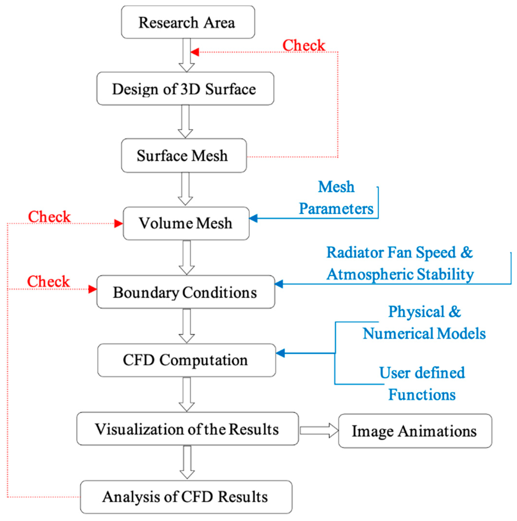
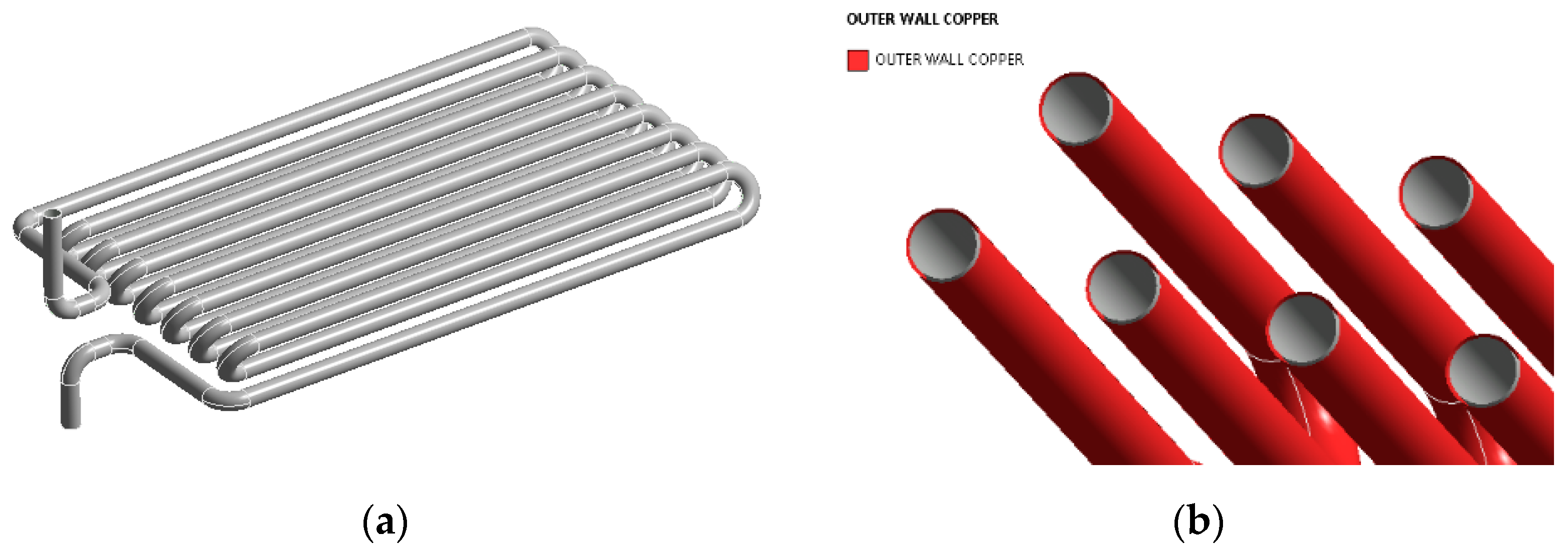
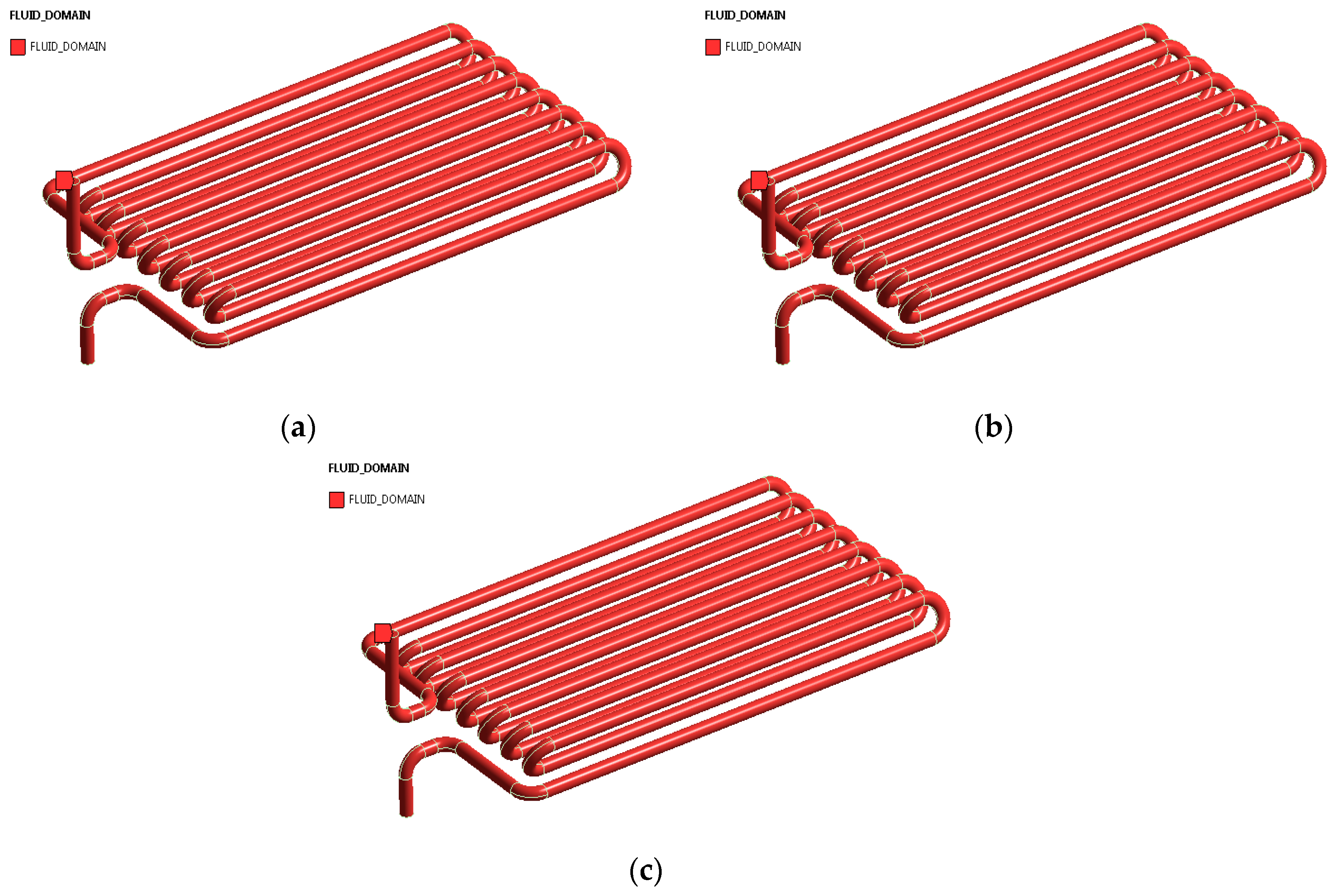
The CFD analysis methodology is shown in Figure 6. According to the dimensions presented in Figure 5, the geometry was made using ANSYS Design Modeler, and the resulting 3D model and cut section view is presented in Figure 7.

12. Optimization of Temperature

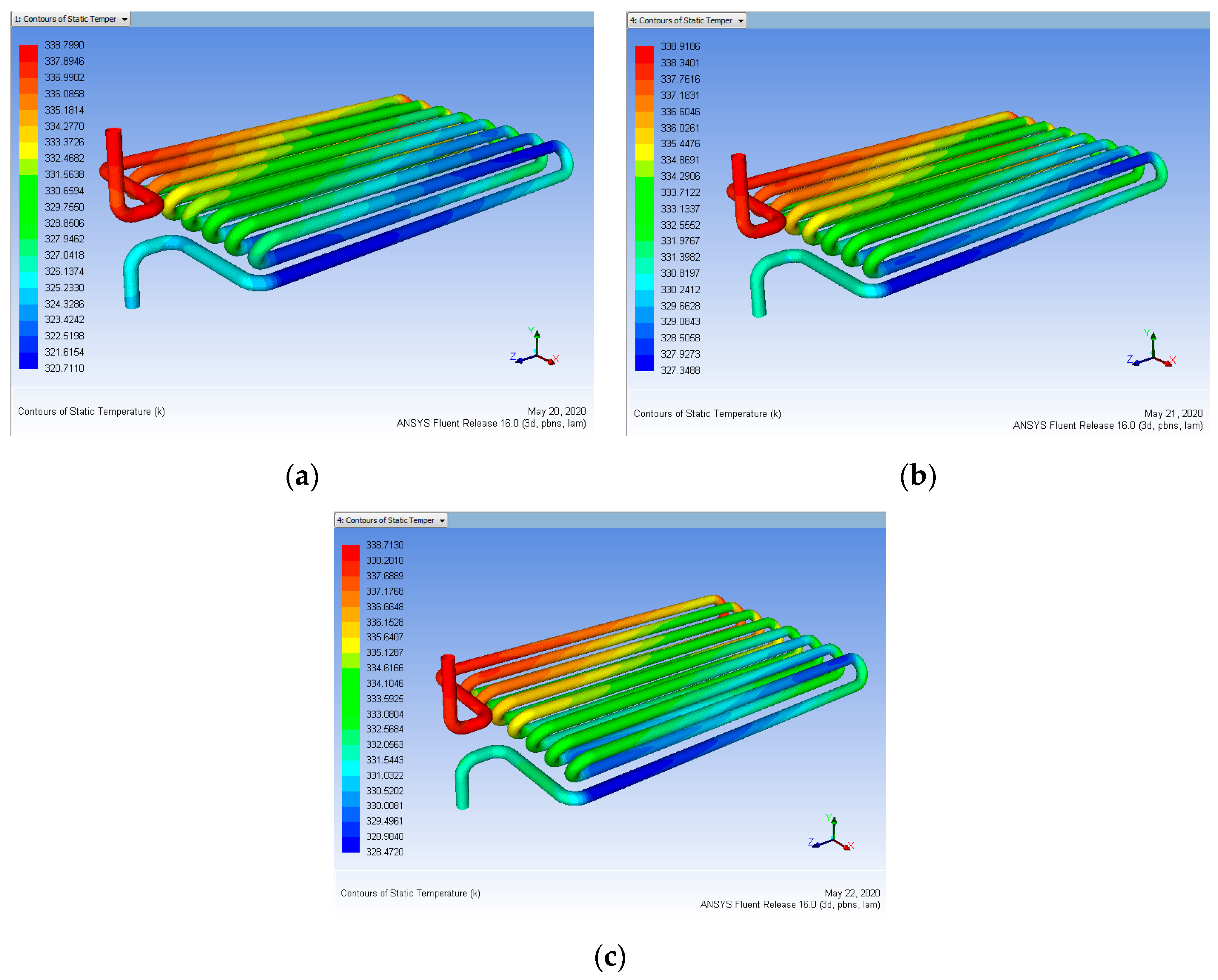
Based on the nine cases obtained in the orthogonal array in Table 2, the simulation was carried out in CFD for three levels of temperature as heat input, three levels of the mass flow rate of coolant fluid transmitted, and three different levels of coating thickness, as shown in Figure 8a–c.
To proceed with the Fluent setup, it was necessary to know the flow regime of the fluid. For this purpose, the Reynolds Number, Re, was calculated as follows:
R e = 4   ·   m ˙ π   ·   μ   ·   D
where m ˙ is the mass flow rate of water, μ is the viscosity of water, and D is the inner pipe diameter. Substituting the known values:
R e = 4 × 0.05 π × 0.001003 × 9 × 10 3 = 7052.40
Since the Reynolds number is higher than 4000, the fluid flow can be considered as turbulent. Consequently, the Fluent setup was initialized, and the energy equation was activated. The selected viscous model was k-ε realizable, with enhanced wall treatment and thermal effects activated [26,27]. The working fluid was as specified as water, and the solids were aluminum and copper. Moreover, the boundary conditions were specified. The “Inlet” named selection received a boundary condition of “mass-flow-inlet”, with a magnitude of 0.15, 0.30, and 0.45 L/min along positive z-direction and a temperature of 323, 343, and 363 K. The “Outlet” named selection was specified as a “pressure-outlet” with 0 Pa gauge. The “Symmetry” named selection received the condition of “symmetry” and the “Convection” named selection received a “wall” condition subjected to convection, with a free stream temperature of 298 K and a convective heat transfer coefficient of 450 W m−2 K−1.
Furthermore, the solution scheme SIMPLEC was activated, and it was considered a spatial discretization of second order upwind for the energy, pressure, and momentum equations. The residuals convergence limits were specified as 1 × 10⁻⁶, and consequently, a hybrid initialization was carried out [28,29]. The simulation was executed for a maximum of 3000 iterations, and convergence was reached after approximately 1200 iterations for all the cases.
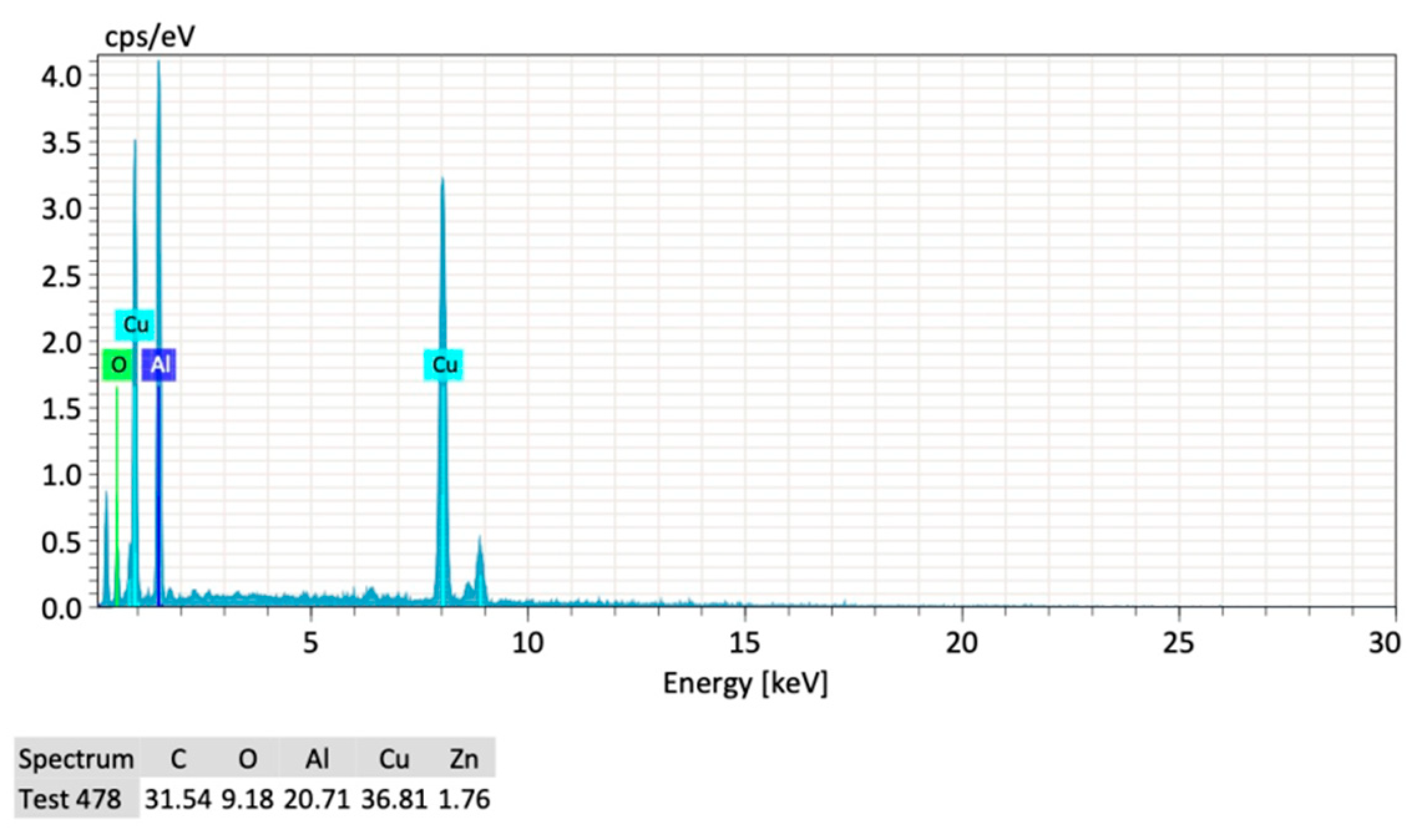
Figure 9 shows the SEM images of the samples coated surface. In Figure 10, The Y-axis shows counts and the X-axis shows the X-ray energy. The location of the summit helps to identify the elements and the maximum height helps to assess the concentration of each element. Table 5 shows the test results of the EDX of the coated surface.

13. Data Analysis

Within this research, the key effects of the heat pipe activity parameters are calculated, the variance analysis (ANOVA) performed, and optimum conditions based on the Taguchi method defined. As seen in Figure 8a–c, key effects are used for the heat pipe analyzing to analyze the impacts of each element. The experiment of the L9 is capable of computing the efficiency of the heat pipe (ANOVA-significant factor) using the observations effectiveness, rate of heat transfer, and overall heat transfer co-efficient of Table 6. CFD Analysis readings for 323 K are listed in Table 7, ANOVA responses and means results are given respectively in Table 8 and Table 9. CFD Analysis readings for 343 K are listed in Table 10, ANOVA responses and means results are given respectively in Table 11 and Table 12. CFD Analysis readings for 363 K are listed in Table 13, ANOVA responses and means results are given respectively in Table 14 and Table 15 in terms of effectiveness, rate of heat transfer, and overall coefficient of heat transfer and each of the values are observed.

14. Results & Discussion

14.1. Case 1: (Heat Input = 323 K)

Based on the nine orthogonal cases of Table 2, simulation in CFD for the provided heat input 323 K and three different thicknesses for the coating and three various flow rates of fluid were performed in CFD.
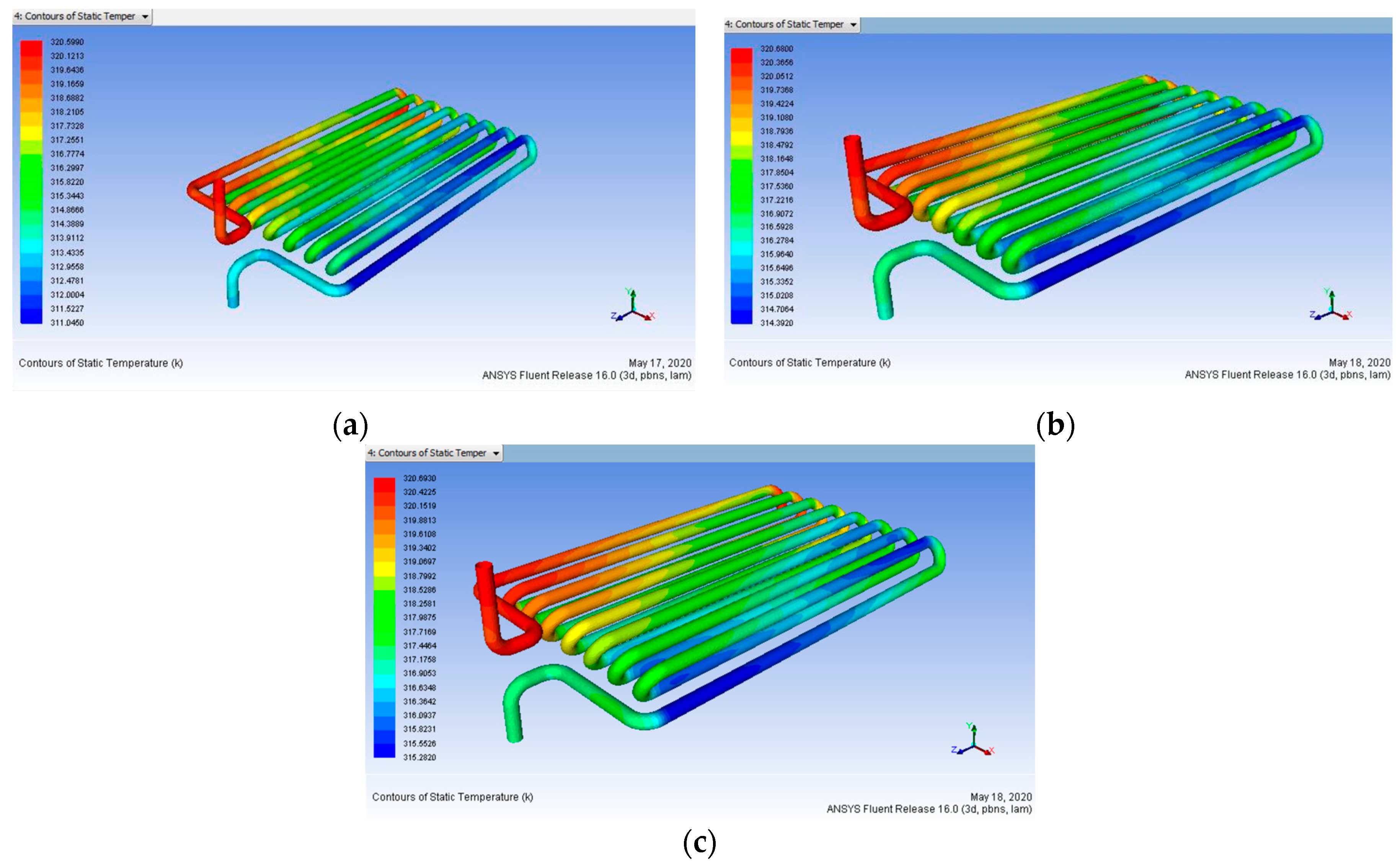
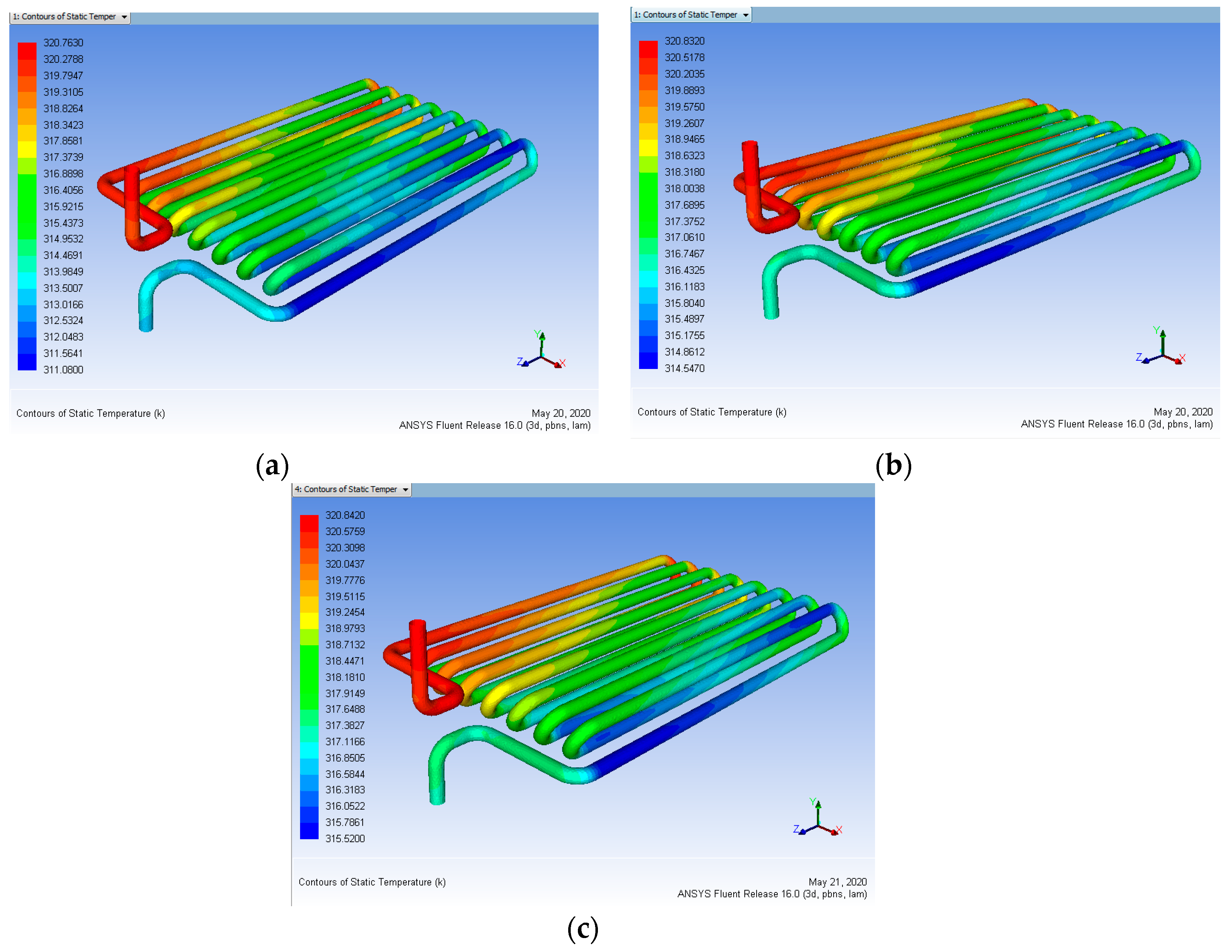
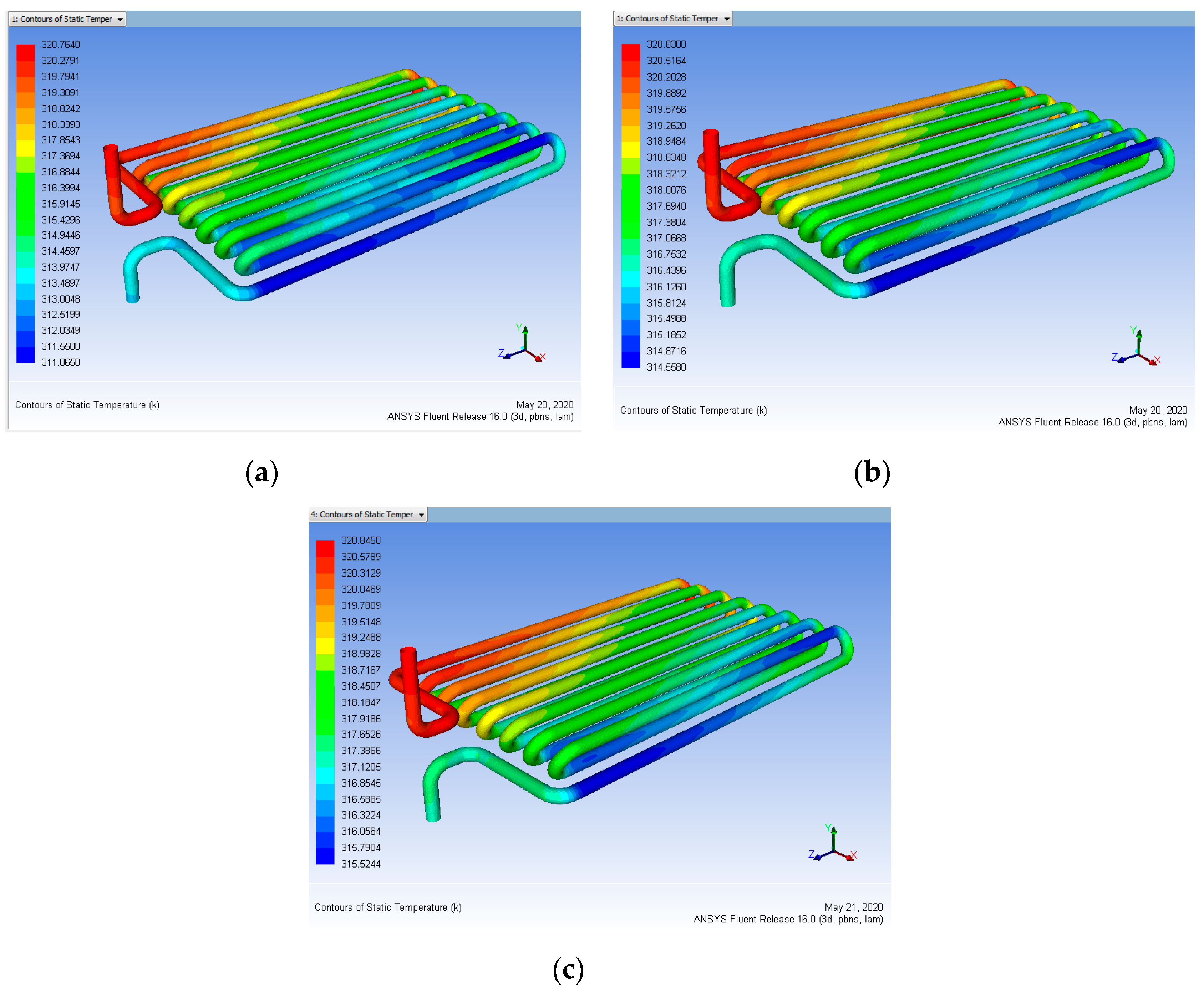
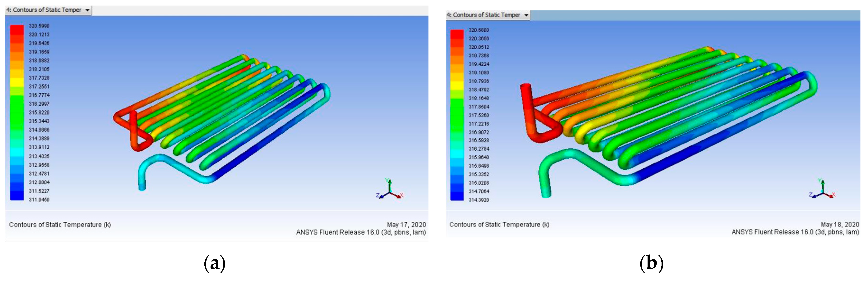
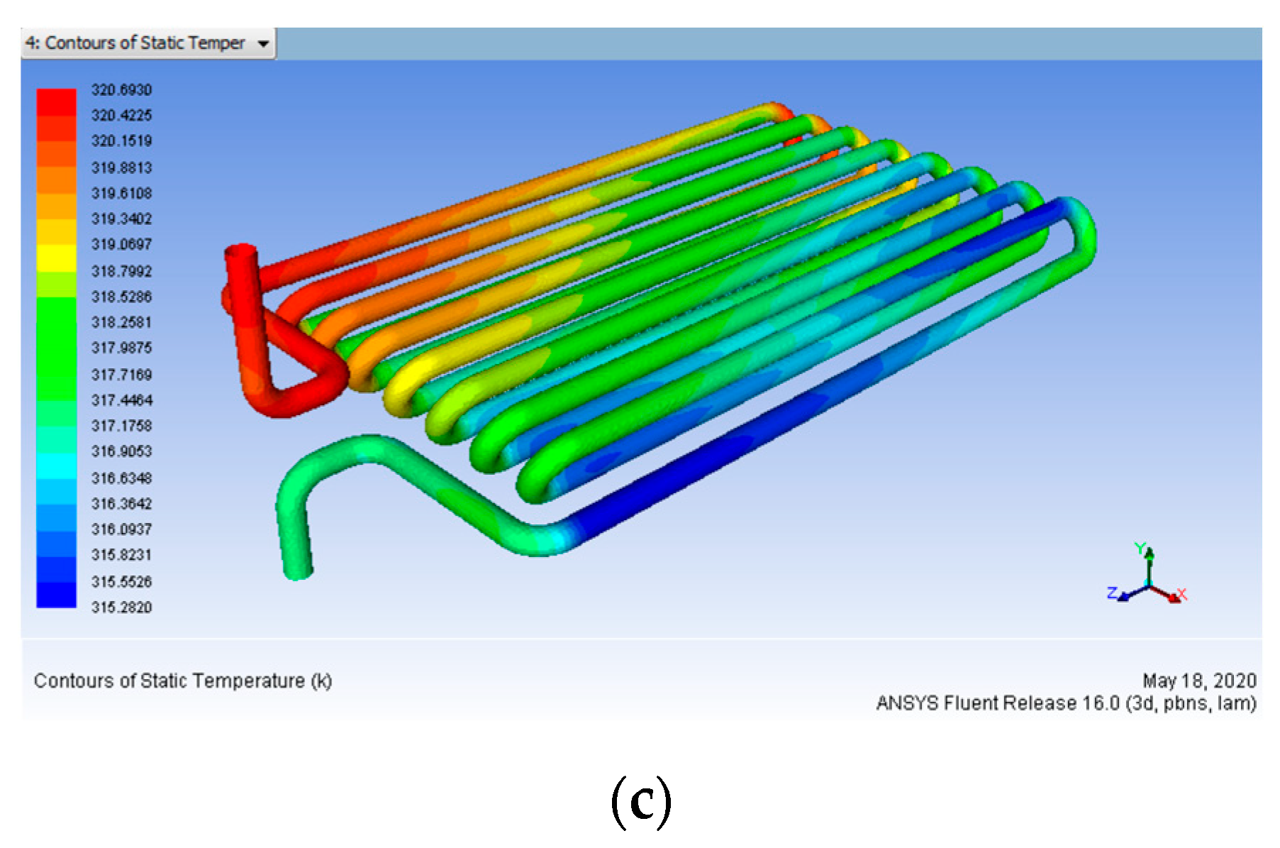
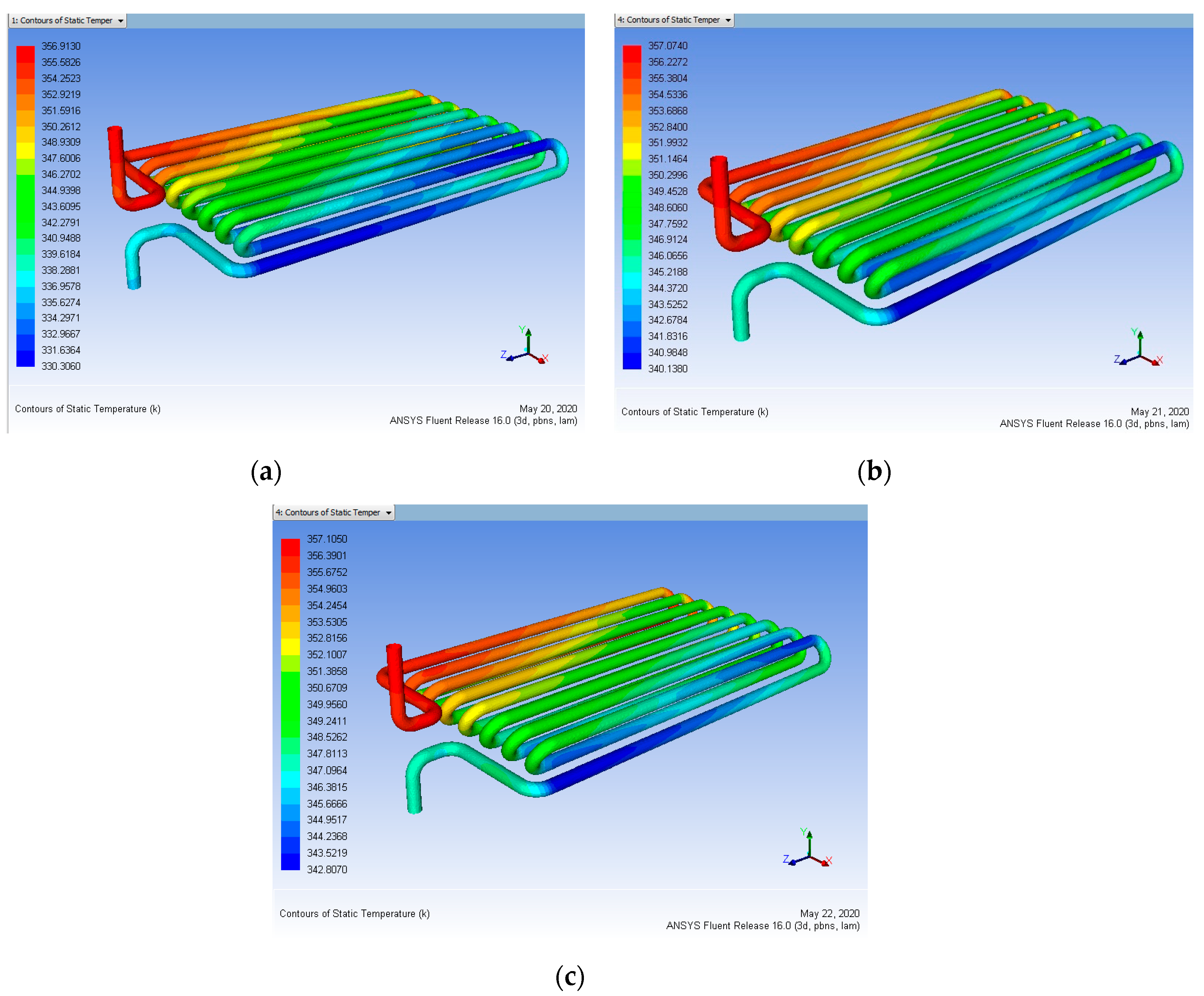
The effect of the coating of each element at various conditions is seen in Figure 11, Figure 12, Figure 13 and Figure 14 They prove that, with all three parameters, the efficiency of nano-coated tubes improves the characteristics of heat transfer. In Table 7, it can be observed that 100 μm of maximum coating thickness yield is higher and a minimum mass flow rate of 0.15 L/min is fine. So, the difference between the heat output without coating and with coating is 4.073 K.
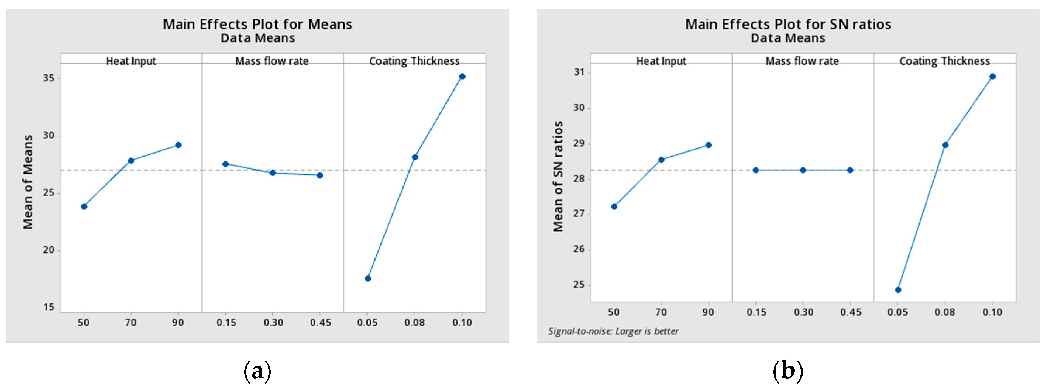
The result of the main effects plot for means and SN ratios from each element to specific level conditions is seen in Figure 15. This indicates that for all three parameters, heat input, mass flow rate, and thickness of the coating. We observed that the overall coefficient of heat transfer and effectiveness of the nano-coated tubes is obviously increasing. The overall heat transfer and effectiveness are higher for 100 µm thickness and increases the overall heat transfer and effectiveness while the mass flow rate is 0.15 L/min.

14.2. Case 2: (Heat Input = 343 K)

Based on the nine orthogonal cases of Table 2, simulation in CFD for the provided heat input 343 K and three different thicknesses for the coating and three various flow rates of fluid were performed in CFD.
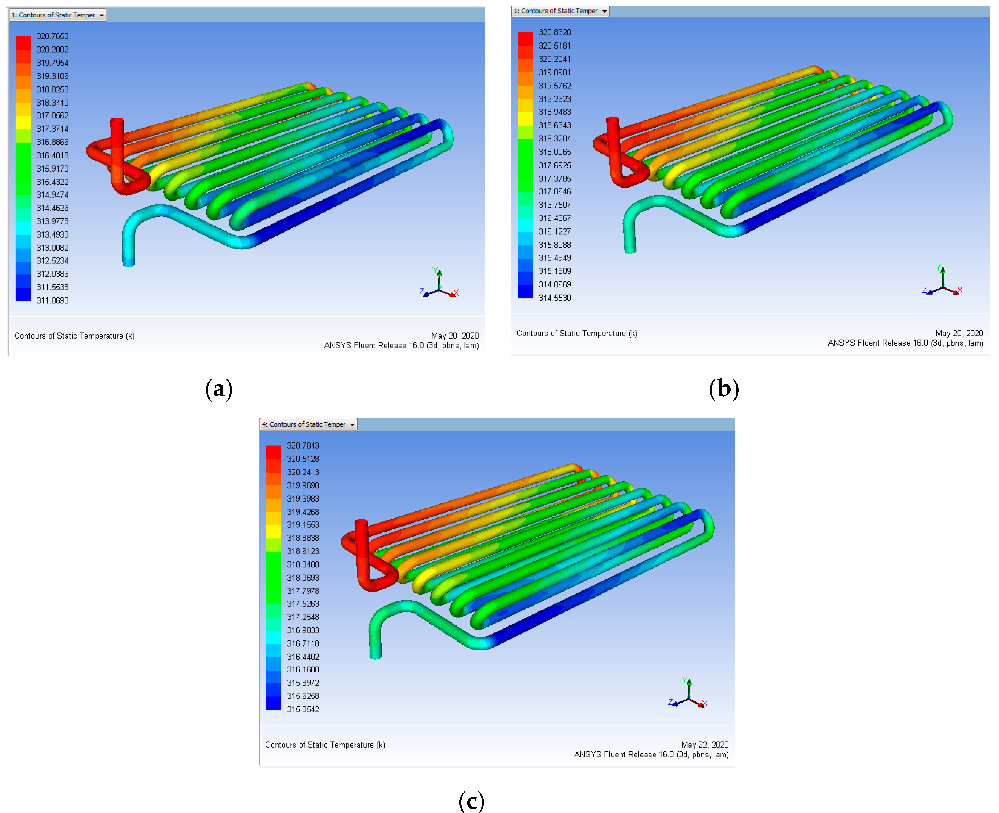
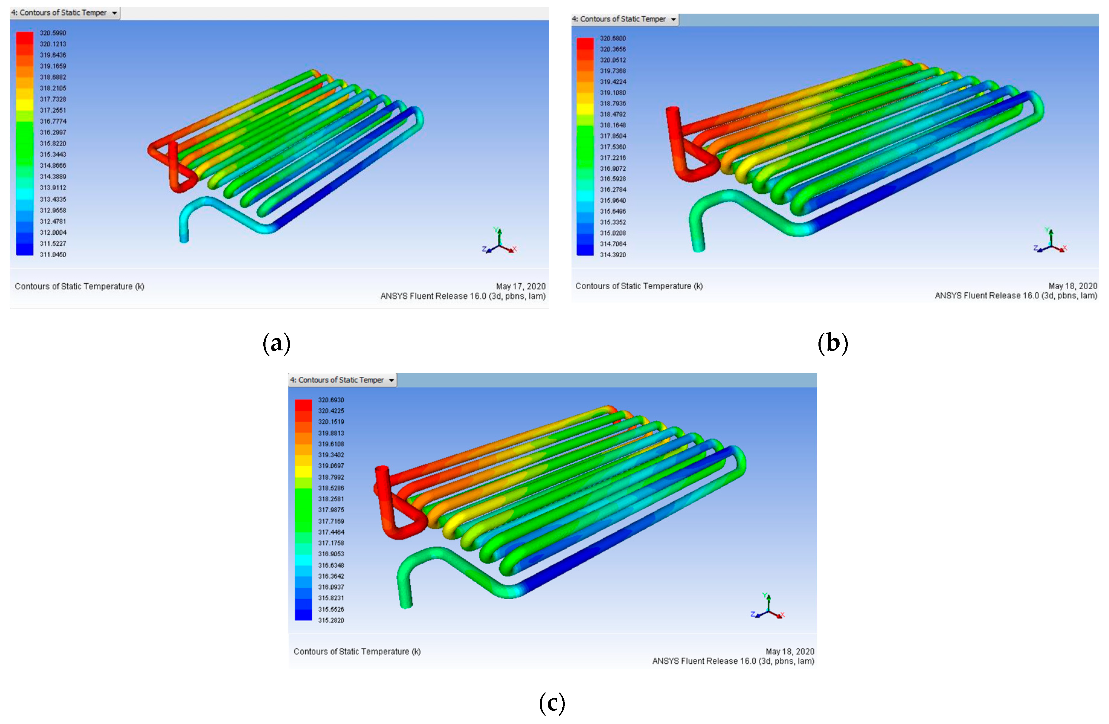
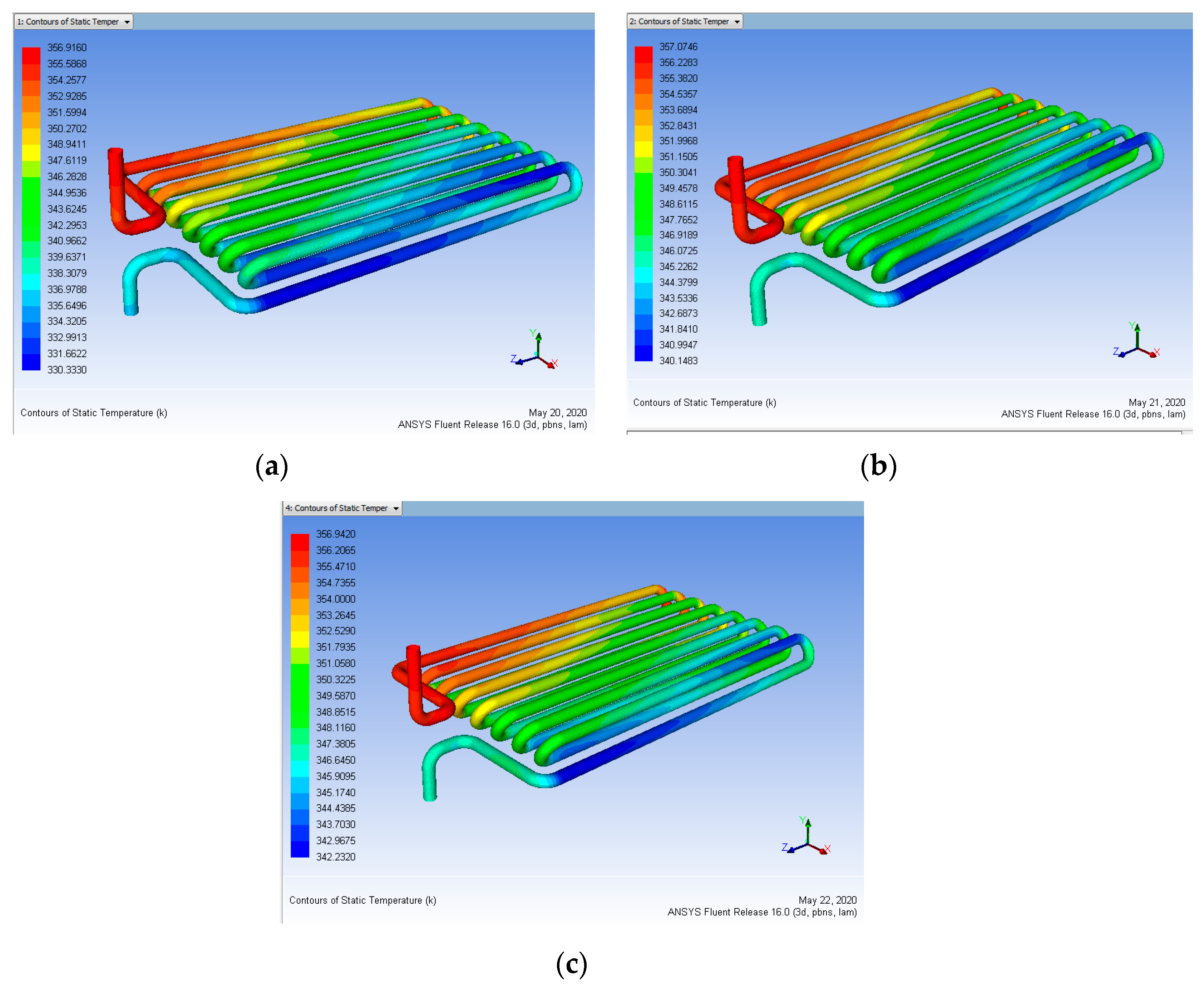
The effect of the coating of each element at various conditions is seen in Figure 16, Figure 17, Figure 18 and Figure 19. They prove that, with all three parameters, the efficiency of nano-coated tubes improves the characteristics of heat transfer. In Table 10, we observe that 100 μm of maximum coating thickness yield is higher and a minimum mass flow rate of 0.15 L/min is fine. So, the difference between the heat output without coating and with coating is 6.478 K.
The result of the main effects plot for means and SN ratios from each element to specific level conditions is seen in Figure 20. This indicates that, for all three parameters, namely heat input, mass flow rate, and thickness of the coating, we observed that the overall coefficient of heat transfer and effectiveness of the nano-coated tubes is obviously increasing. The overall heat transfer and effectiveness are higher for 100 µm thickness and increases the overall heat transfer and effectiveness while the mass flow rate is 0.15 L/min.

14.3. Case 3: (Heat Input = 363 K)

Based on the nine orthogonal cases of Table 2, simulation in CFD for the provided heat input 363 K and three different thicknesses for the coating and three various flow rates of fluid were performed in CFD.
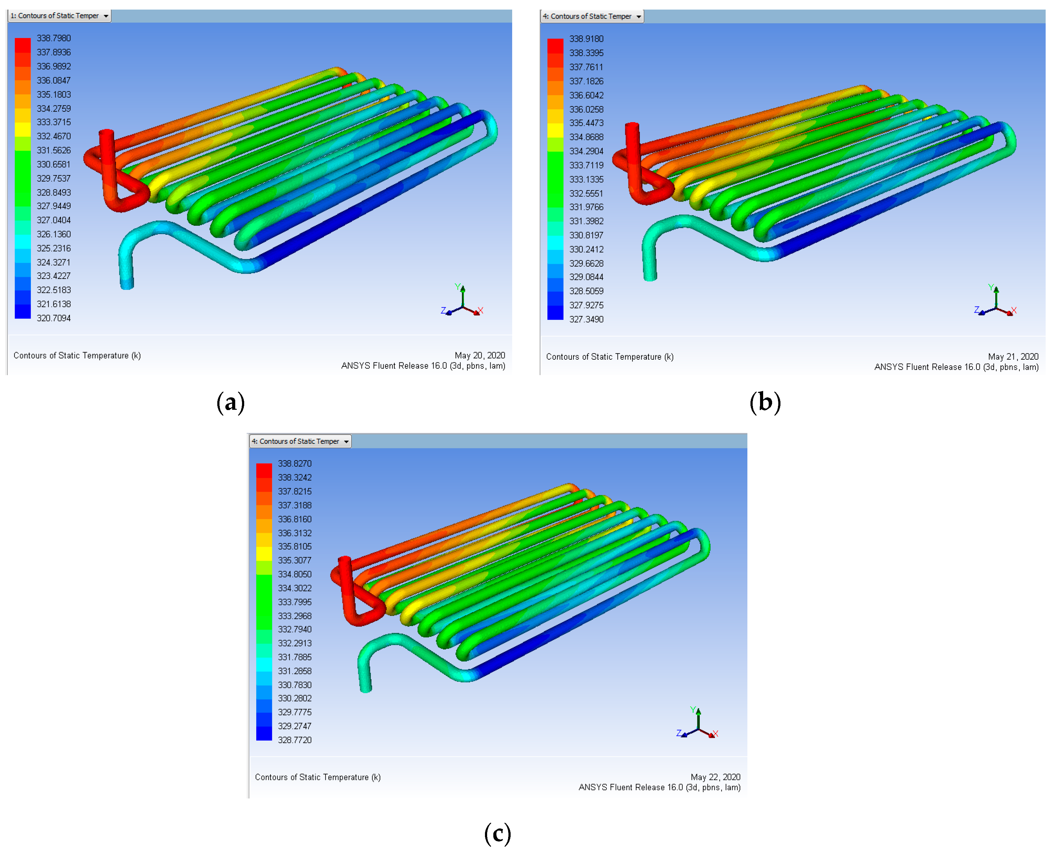
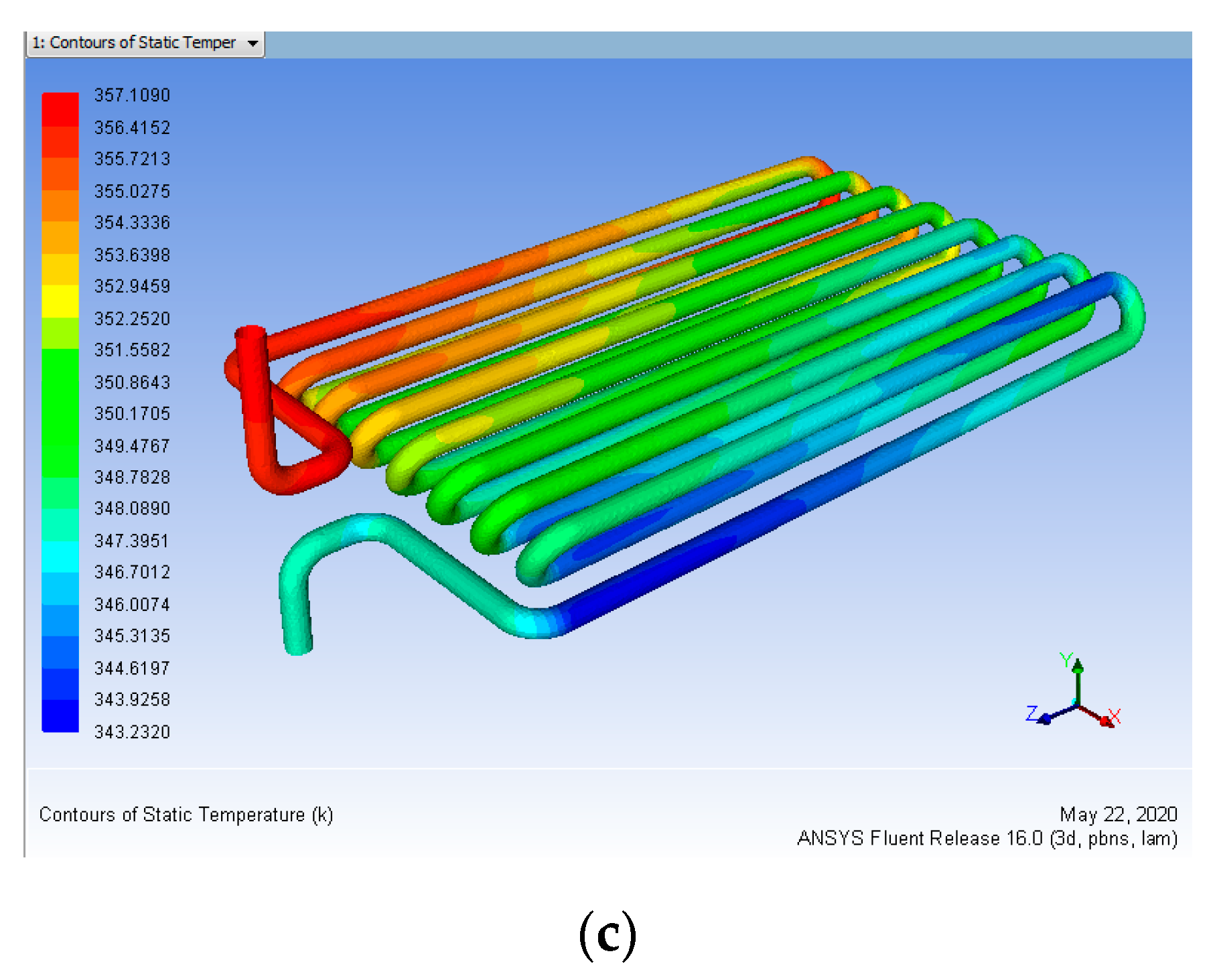
The effect of the coating of each element at various conditions is seen in Figure 21, Figure 22, Figure 23 and Figure 24. This proves that, with all three parameters, the efficiency of nano-coated tubes improves the characteristics of heat transfer. From Table 13, we observed that 100 μm of maximum coating thickness yield is higher and a minimum mass flow rate of 0.15 L/min is fine. So, the difference between the heat output without coating and with coating is 7.1651 K.
The result of the main effects plot for means and SN ratios from each element to specific level conditions is seen in Figure 25. This indicates that for all three parameters, heat input, mass flow rate, and thickness of the coating. We observed that the overall coefficient of heat transfer and effectiveness of the nano-coated tubes is obviously increasing. The overall heat transfer and effectiveness are higher for 100 µm thickness and increases the overall heat transfer while the mass flow rate is 0.15 L/min.

15. Prediction of Optimum Results

Using the Taguchi methodology to determine ideal working parameters for nano-coated pipes, the measurements are carried out and the results are shown in Table 16.

16. Conclusions

The findings for the monitoring of the nano-coated pipe efficiency after the tests are described as follows.
  • The A1 B3 C2 of Taguchi analysis is found to be the optimum operating parameter level for temperature.
  • 100 µm nano-coated pipes have higher heat transfer coefficients at all rates.
  • For maximum temperature as heat input, 0.15 litre/min mass flow rate of coolant fluid conducted more heat.
  • Optimal solutions using the Taguchi method provide better results for nano-coated pipes operations and the number of experiments required to find its efficiency metrics.
  • Findings from experiments show that heat input, mass flow rate, and coating thickness play a significant role in the nano-coated pipe operations.
The design parameters of the Taguchi method and the CFD analysis are found to provide a simple, systematic, and efficient methodology for optimizing process parameters. The findings of ANOVA showed 95% confidence and were confirmed in the most significant parameters. The heat transfer efficiency of the radiator increases primarily due to the copper nano-coating on the aluminum core of the radiator. Through coating the copper particles on the aluminum tubes, the heat transfer properties of copper are accomplished by the heater core. Therefore, we can minimize the front portion of the vehicle by using a copper-coated aluminium tube radiator instead of a traditional aluminium radiator to cool the engine that produces high power to achieve maximum performance. The inner layer of aluminum has the same traditional properties and the outer layer of copper coating is free from rust and has less weight than the true copper alloy radiator.

Author Contributions

Conceptualization, S.S.P. and C.K.K.; methodology, S.S.P. and C.K.K.; software, S.S.P.; validation, S.S.P.; formal analysis, S.S.P. and C.K.K.; investigation, S.S.P. and C.K.K.; resources, S.S.P.; data curation, S.S.P.; writing—original draft preparation, S.S.P.; writing—review and editing, S.S.P. and C.K.K.; visualization, S.S.P. supervision, C.K.K.; project administration, S.S.P. and C.K.K.; funding acquisition, Not Applicable. All authors have read and agreed to the published version of the manuscript.

Funding

The authors declares that no specific funding received for this research work.

Acknowledgments

This research work was executed at The Nanotechnology Research Centre (NRC), SRM Institute of Science and Technology, Kattankulathur, Kanchipuram (D.T.), Tamil Nadu, Chennai.

Conflicts of Interest

The authors declare that they have no known competing financial interests or personal relationships that could have appeared to influence the work reported in this paper.

Abbreviations

Computational fluid dynamics (CFD), signal-to-noise ratio (SNRA), analysis of variance (ANOVA), design of experiments (DOE), mean square deviation (MSD), signal to noise ratio analysis (SNRA), scanning electron microscope (SEM).

References

  1. Klabunde, K.J. Introduction to Nanotechnology; Wiley: Hoboken, NJ, USA, 2003; pp. 1–13. [Google Scholar]
  2. Bernecki, T. Surface science. In Handbook of Thermal Spray Technology; Davis, R., Ed.; ASM International: Geauga County, OH, USA, 2004; pp. 14–35. [Google Scholar]
  3. Park, K.S.; Won, J.P.; Heo, H.S. Thermal flow analysis of vehicle engine cooling system. KSME Int. J. 2002, 16, 975–985. [Google Scholar] [CrossRef]
  4. Lee, S.H.; Hur, N.; Kang, S. An efficient method to predict the heat transfer performance of a louver fin radiator in an automotive power system. J. Mech. Sci. Technol. 2014, 28, 145–155. [Google Scholar] [CrossRef]
  5. Anand, K.D. Investigation on suitability of Aluminium to Copper in a Radiator. Manuf. Sci. Technol. 2015, 3, 16–23. [Google Scholar]
  6. Bae, K.E.; Chae, K.W. Oxidation behaviour of amorphous boron carbide-silicon carbide nano multi-layer thin films. Surf. Coat. Technol. 2015, 276, 55–58. [Google Scholar] [CrossRef]
  7. Wang, B.; Peng, X. Experimental investigation on liquid forced-convection heat transfer through microchannels. Int. J. Heat Mass Transf. 1994, 37, 73–82. [Google Scholar] [CrossRef]
  8. Rajput, K.A.; Kulkarni, A.V. A Review on Effect of Perforation and Carbon Nanotubes coating on Heat transfer augmentation. Int. J. Innov. Res. Sci. Eng. Technol. 2014, 3, 9412–9415. [Google Scholar]
  9. Sujith, K.C.S.; Suresh, S.; Rajiv, K. Heat transfer enhancement by Nanostructured carbon Nanotube Coating. Int. J. Sci. Res. 2012, 3, 1–5. [Google Scholar]
  10. Josell, D.; Bonevich, J.; Nguyen, T.; Johnson, R. Heat transfer through nanoscale multilayered thermal barrier coatings at elevated temperatures. Surf. Coat. Technol. 2015, 275, 75–83. [Google Scholar] [CrossRef]
  11. Dario, B. Nanostructure coatings remove heat four times faster. N. Atlas Artic. 2018, 7, 15384. [Google Scholar]
  12. Babu, K.A.; Sherjin, P. Experimental investigations of the performance of a thermoacoustic refrigerator based on the Taguchi method. J. Mech. Sci. Technol. 2018, 32, 929–935. [Google Scholar] [CrossRef]
  13. Dar, A.A.; Anuradha, N. Use of orthogonal arrays and design of experiment via Taguchi L9 method in probability of default. Accounting 2018, 4, 113–122. [Google Scholar] [CrossRef]
  14. Chan, Y.H.; Dang, K.V.; Yusup, S.; Lim, M.T.; Zain, A.M.; Uemura, Y. Studies on catalytic pyrolysis of empty fruit bunch (EFB) using Taguchi’s L9 Orthogonal Array. J. Energy Inst. 2014, 87, 227–234. [Google Scholar] [CrossRef]
  15. Pavani, P.N.L.; Rao, R.P.; Srikiran, S. Performance evaluation and optimization of nano boric acid powder weight percentage mixed with vegetable oil using the Taguchi approach. J. Mech. Sci. Technol. 2015, 29, 4877–4883. [Google Scholar] [CrossRef]
  16. Amir, F. Performance characteristics of a concentric annular heat pipe—Part II—Vapour flow analysis. ASME J. Heat Transf. 1989, 111, 847–851. [Google Scholar]
  17. Thomas, V.H. Orthogonal array experiment in systems engineering and architecting. Syst. Eng. 2011, 14, 208–222. [Google Scholar]
  18. Athreya, S.; Venkatesh, Y.D. Application of Taguchi method for optimization of process parameters in improving the surface roughness of lathe facing operation. Int. Ref. J. Eng. Sci. 2012, 1, 13–19. [Google Scholar]
  19. Amir, F. Heat Pipe Science and Technology; Taylor & Francis: Washington, DC, USA, 1995. [Google Scholar]
  20. Chandourene, S.; Gruss, A. Theoretical and experimental study of high temperature heat pipe heat exchanger application to 1300kW respirator. In Proceedings of the Sixth International Heat Pipe Conference, Grenoble, France, 25–29 May 1987. [Google Scholar]
  21. Kaminaga, F.; Hashimoto, H.; Feroz, C.; Goto, K.; Masumura, K. Heat transfer characteristics of evaporation and condensation in a two-phase closed thermosyphon. In Proceedings of the 10th International Heat Pipe Conference, Stuttgart, Germany, 21–25 September 1997; pp. 1–6. [Google Scholar]
  22. Mariya, I.; Yvan, A. Christian schaeffer, jean-bernard dezord, and juergen schulz-harder, heat pipe integrated in Direct Bonded Copper (DBC) technology for cooling of power electronics packaging. IEEE Trans. Power Electron. 2006, 21, 1541–1547. [Google Scholar]
  23. Lee, K.-H.; Yi, J.-W.; Park, J.-S.; Park, G.-J. An optimization algorithm using orthogonal arrays in discrete design space for structures. Finite Elem. Anal. Des. 2003, 40, 121–135. [Google Scholar] [CrossRef]
  24. Merton, R.C. On the pricing of corporate debt: The risk structure of interest rates. J. Financ. 1974, 29, 449. [Google Scholar] [CrossRef] [Green Version]
  25. Sonan, R.; Harmand, S.; Pelle, J.; Léger, D.; Fakès, M. Transient thermal and hydrodynamic model of flat heat pipe for the cooling of electronics components. Int. J. Heat Mass Transf. 2008, 51, 6006–6017. [Google Scholar] [CrossRef]
  26. Hull, J.C.; Basu, S. Options, Futures and Other Derivatives; Pearson Education India: Chennai, India, 2016. [Google Scholar]
  27. Ranjit, K.R. Design of Experiments Using the Taguchi Approach; John Wiley & Sons: New York, NY, USA, 2001. [Google Scholar]
  28. Oliet, C.; Oliva, A.; Castro, J.; Perez-Segarra, C.-D. Parametric studies on automotive radiators. Appl. Therm. Eng. 2007, 27, 2033–2043. [Google Scholar] [CrossRef]
  29. Upendra, K. CFD analysis of automobile radiator—A review. In Proceedings of the International Journal of Engineering Research and Applications, International Conference on Emerging Trends in Mechanical and Electrical Engineering, Thai Nguyen, Vietnam, 13–14 March 2014. [Google Scholar]
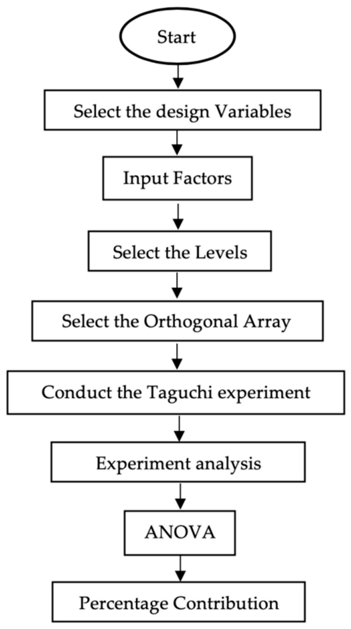
Figure 1. Flow chart–Process of Taguchi Analysis.
Coatings 10 00804 g001
Figure 2. Experimental schematic diagram and Thermocouple Position in Radiator.
Coatings 10 00804 g002
Figure 3. Experiment-Radiator Thermal analysis.
Coatings 10 00804 g003
Figure 4. (a) Mesh Created; (b) Zoomed View; (c) Geometry Statistics.
Coatings 10 00804 g004
Figure 5. Principal tube dimensions.
Coatings 10 00804 g005
Figure 6. Methodology.
Coatings 10 00804 g006
Figure 7. (a) Aluminium Radiator (Before coating) and (b) Copper Coated Cut Section View.
Coatings 10 00804 g007
Figure 8. (a) 50 µm, (b) 80 µm, (c) 100 µm copper coating on Aluminium Radiator tubes.
Coatings 10 00804 g008
Figure 9. SEM image of coating material (Characterization facility. SRMIST, Chennai). (a) 50 µm; (b) 80 µm; (c) 100 µm.
Coatings 10 00804 g009
Figure 10. Typical EDX spectrum.
Coatings 10 00804 g010
Figure 11. Heat input 323 K vs. mass flow rate (a) 0.15, (b) 0.30, (c) 0.45 L/min (Before Coating).
Coatings 10 00804 g011
Figure 12. Heat input 323 K vs. Coating Thickness 50 µm for mass flow rate (a) 0.15, (b) 0.30, (c) 0.45 L/min (After Coating).
Coatings 10 00804 g012
Figure 13. Heat input 323 K vs. Coating Thickness 80 µm for mass flow rate (a) 0.15, (b) 0.30, (c) 0.45 L/min (After Coating).
Coatings 10 00804 g013
Figure 14. Heat input 323 K vs. Coating Thickness 100 µm for mass flow rate (a) 0.15, (b) 0.30, (c) 0.45 L/min (After Coating).
Coatings 10 00804 g014
Figure 15. Taguchi Analysis for Rate of heat transfer Versus Heat Input, Mass Flow Rate and Coating Thickness. (a) Main Effects Plot for Means; (b) Main Effects Plot for SN ratios.
Coatings 10 00804 g015
Figure 16. Heat input 343 K vs. mass flow rate (a) 0.15, (b) 0.30, (c) 0.45 L/min (Before Coating).
Coatings 10 00804 g016
Figure 17. Heat input 343 K vs. Coating Thickness 50 µm for mass flow rate (a) 0.15, (b) 0.30, (c) 0.45 L/min (After Coating).
Coatings 10 00804 g017
Figure 18. Heat input 343 K vs. Coating Thickness 80 µm for mass flow rate (a) 0.15, (b) 0.30, (c) 0.45 L/min (After Coating).
Coatings 10 00804 g018
Figure 19. Heat input 343 K vs. Coating Thickness 100 µm for mass flow rate (a) 0.15, (b) 0.30, (c) 0.45 L/min (After Coating).
Coatings 10 00804 g019
Figure 20. Taguchi Analysis for Effectiveness Versus Heat Input, Mass Flow Rate and Coating Thickness. (a) Main Effects Plot for Means; (b) Main Effects Plot for SN ratios.
Coatings 10 00804 g020
Figure 21. Heat input 363 K vs. mass flow rate (a) 0.15, (b) 0.30, (c) 0.45 L/min (Before Coating).
Coatings 10 00804 g021aCoatings 10 00804 g021b
Figure 22. Heat input 363 K vs. Coating Thickness 50 µm for mass flow rate (a) 0.15, (b) 0.30, (c) 0.45 L/min (After Coating).
Coatings 10 00804 g022
Figure 23. Heat input 363 K vs. Coating Thickness 80 µm for mass flow rate (a) 0.15, (b) 0.30, (c) 0.45 L/min (After Coating).
Coatings 10 00804 g023
Figure 24. Heat input 363 K vs. Coating Thickness 100 µm for mass flow rate (a) 0.15, (b) 0.30, (c) 0.45 L/min (After Coating).
Coatings 10 00804 g024aCoatings 10 00804 g024b
Figure 25. Taguchi Analysis for Overall heat transfer Versus Heat Input, Mass Flow Rate and Coating Thickness. (a) Main Effects Plot for Means; (b) Main Effects Plot for SN ratios.
Coatings 10 00804 g025
Table 1. Parameters for control (Design factors) and their Levels.
Control ParametersLevel_OneLevel_TwoLevel_Three
Heat input (K)323343363
Mass flow rate (L/min)0.150.300.45
Coating thickness (µm)5080100
Table 2. Three level considerations Orthogonal Array for L9.
ConditionLevel_OneLevel_TwoLevel_Three
OneOneOneOne
TwoOneTwoTwo
ThreeOneThreeThree
FourTwoOneTwo
FiveTwoTwoThree
SixTwoThreeOne
SevenThreeOneThree
EightThreeTwoOne
NineThreeThreeTwo
Table 3. Engine and Radiator Specification.
Engine SpecificationRadiator Specification
TypeWater Cooled Sohc EngineRadiator’s TypeCompact Heat Exchanger-Circular
Tube with Continuous Fin
Fuel UsedPetrolRadiator’s VolumeP × L × T = 500 × 30 × 550 mm3
Max. Power (bhp@rpm)37bhp @5000 rpmTube Diameter10 mm
Engine Displacement796 CCTube Length330 mm
Max. Torque59 nm @2500 rpmNumber of Row2
No. of Cylinders4Number of tubes per Row8
No. of valves2 valves/cylinderPit Length11 mm
Valve Train SohcMaterialCoper coated Aluminium tubes
Fuel trainMpfiFin MaterialAluminium
Pressure Ratio8.8:1Fin thickness0.1 mm
Table 4. Material properties.
MaterialThermal Conductivity
(W m−1 K−1)
Density
(kg/m3)
Specific Heat
(J kg−1 K−1)
Viscosity
(kg m−1 s−1)
Aluminium1902719871-
Copper4013210385-
Water0.6998.241820.001003
Table 5. EDX Test Results.
ElementAt. No.Mass [%]Mass Norm [%]Atom [%]Abs. Error [%]
(1 Sigma)
Rel. Error [%]
(1 Sigma)
Cu2941.2736.8112.671.072.59
C635.3631.5457.426.5118.40
Al1323.2220.7116.781.225.25
O810.299.1812.552.1621.02
Zn301.971.760.590.105.04
112.11100.00100.00
Table 6. Experimental Design for L9 Orthogonal Array.
No. of TestHeat Input
(K)
Mass Flow Rate
(L/min)
Coating Thickness
(µm)
Rate of Heat Transfer
(kW)
SNRAEffectivenessSNRAOverall Heat Transfer Coefficient
(W m−2 K−1)
SNRA
13230.15503.149.9415.6023.86270.4548.64
23230.30805.0214.0124.9627.94459.2953.24
33230.451006.2715.9531.1929.88598.5255.54
43430.158011.7021.3629.1129.281284.5262.17
53430.3010014.6323.3036.3931.211687.864.54
63430.45507.3217.2918.2025.20746.8257.46
73630.1510022.9927.2338.1331.622816.5668.99
83630.305011.5021.2119.0625.601238.1161.85
93630.458018.3925.2930.5029.682135.8966.59
Table 7. CFD Analysis Reading for 323 K.
Coating ThicknessMass Flow RateHeat Input
(K)
Heat Output (Without Coating) (K)Heat Output (With Coating) (K)
500.15323314.5623311.6682
80323311.2169
100323310.4896
500.30323315.9843312.1283
80323311.8257
100323311.2673
500.45323317.2348312.2314
80323311.9846
100323311.4213
Table 8. Response Table for SNRA.
LevelHeat InputMass Flow RateCoating Thickness
113.3019.5116.15
220.6519.5120.22
324.5819.5122.16
Delta11.280.006.01
Rank132
Table 9. Table of responses for means.
LevelHeat InputMass Flow RateCoating Thickness
14.81012.6107.320
211.21710.38311.703
317.62710.66014.630
Delta12.8172.2277.310
Rank132
Table 10. CFD Analysis Reading for 343 K.
Coating ThicknessMass Flow RateHeat Input
(K)
Heat Output (Without Coating)
(K)
Heat Output (With Coating)
(K)
500.15343328.2653324.1464
80343323.6230
100343321.7859
500.30343330.8934325.1792
80343324.6932
100343323.9572
500.45343332.3284325.8741
80343324.7642
100343323.1260
Table 11. Response Table for SNRA.
LevelHeat InputMass Flow RateCoating Thickness
127.2328.2624.89
228.5728.2628.97
328.9728.2630.91
Delta1.740.006.02
Rank132
Table 12. Table of responses for means.
LevelHeat InputMass Flow RateCoating Thickness
123.9227.6117.62
227.9026.8028.19
329.2326.6335.24
Delta5.310.9817.62
Rank132
Table 13. CFD Analysis Reading for 363 K.
Coating ThicknessMass Flow RateHeat Input
(K)
Heat Output (Without Coating) (K)Heat Output (With Coating) (K)
500.15363341.1494339.1287
80363336.8967
100363333.9843
500.30363344.8634340.1275
80363337.1278
100363334.9483
500.45363347.9631341.4793
80363338.4752
100363336.6382
Table 14. Response Table for SNRA.
LevelHeat InputMass Flow RateCoating Thickness
152.4859.9455.99
261.4059.8860.67
365.8159.8763.03
Delta13.340.077.04
Rank132
Table 15. Table of responses for means.
LevelHeat InputMass Flow RateCoating Thickness
1442.801457.20751.8
21239.71128.41239.2
32063.51160.41701.00
Delta1620.80328.80949.20
Rank132
Table 16. Measurements Results.
Heat InputMass Flow RateCoating ThicknessPSNRAPMEANS
3230.155048.6098154.40
3230.308053.2362367.06
3230.4510055.5790806.80
3430.158062.21231492.80
3430.3010064.51451571.75
3430.455057.4588654.59
3630.1510068.98892724.33
3630.305061.89261446.39
3630.458066.55962019.84