Experimental Observation of Flow Reversal in Thin Liquid Film Flow Falling on an Inclined Plate

Abstract

A customized particle image velocimetry/planar laser induced fluorescence (PIV/PLIF) experimental method, aiming to capture transient hydrodynamics of solitary waves of inertia-dominated falling liquid films, is presented in this paper. A novel PIV/PLIF technique, which only uses one camera to capture simultaneously both particle image and fluorescence, and meanwhile a post-processing imaging method is also developed, which is able to simultaneously measure both internal velocity field in film and its topology. To validate the fidelity of the novel PIV/PLIF technique, a comparison between experimental results of streamwise velocity profile and film thickness and that of the Nusselt’s prediction at low Reynold number is carried out, and in addition, integral continuity is checked for transient wavy film, both of which shows that they are in good agreement. Based on experimental velocity fields and film topology, pressure distribution inside film is derived with the Poisson equation. Considering characteristics of traveling waves, the experimental results are presented respectively in spatial mode and temporal mode. In spatial mode, capillary wave dynamics are demonstrated out of velocity field, film topology and pressure distribution, which reveals that flow reversal occurs at capillary troughs. In temporal mode, the mechanism of flow reversal at capillary troughs is scrutinized on the basis of high-frequency velocity sampling and the derived pressure gradient. It is shown that flow reversal at capillary troughs is triggered due to occurrence of positive pressure gradient at the back side of the capillary wave crest, rather than the trough upstream as stated by the previous researchers. By elucidating the dynamics of flow reversal, mechanisms for the upper limit of Reynold number with respect to flow reversal underneath capillary wave trough were proposed, which might be the gradually saturated deceleration from the capillary curvature and shorten deceleration duration determined by the wave speed and capillary wave length. Our results should be of interest for optimization of the mass transport model of falling liquid films and shed light on the revealing of flow reversal mechanism.

1. Introduction

Liquid film flow has a large surface volume ratio, which can render high capacity of energy transportation considering its liquid volume, resulting wide usages in engineering fields [1,2]. For film flow, the surface topology not only indicates the instability dynamics, but also influences the transport process underneath. Observation for spatial-temporal velocity field, even possible multiple fields, could give promising experimental insights into film flow.

The multiphase dynamics of liquid film has been investigated by many researchers with experimental approaches since the pioneering work by Kapitza [3]. Since researches in this article focused on experimental outcomes of solitary wave dynamics, especially velocity fields in solitary waves. The literature review mainly focuses on non-intrusive application of falling liquid film and flow reversal in solitary waves.

As experimental measurement technologies develop, new emerging non-intrusive measurement techniques could complete film experiments with better performance and less influence. On the numerical simulation side, especially for the transport process inside the film, it requires more than film thickness time traces data to validate the models, experimental results of velocity with correlating topology also become indispensable for further validation.

Non-intrusive velocity measurement techniques used in experiments were mainly laser doppler velocimetry (LDV) and PIV. LDV is a point wise sample at a certain position, which could not resolve the instantaneous velocity profile or instantaneous velocity field. For film flow, the PIV technique was initially applied with cylinder sub-plate, which can easily guarantee measurement plane parallel to the tube axis and extends normally to the tube wall.

For example, rather early attempts to investigate the velocity field structure in the film cross section was done by Adomeit [4], who used a camera to record the flow path lines of particles in film and observed a looped shaped flow path, which showed a backflow phenomenon. In his experiment, a glass tube was used with matched index of the refraction technique.

Alekseenko [5] applied PIV to investigate the velocity field in film flowing down an inclined cylinder, in experiments, he carried out a special calibration method with restrictions of film surface shape staying almost unchanged. Dietze [6,7,8] applied both LDV and PIV to investigate falling annular film flow with a special designed cuboid test section, and flow reversal phenomena were observed in the capillary wave region while the results of velocity filed was derived without rigorous calibration. Ashwood [9] also used PIV to investigated velocity profiles within the liquid film of the vertical square two-phase flow.

The above PIV applications can be catalogued into micro-PIV, due to its high optical magnification in image acquisition, which allowed for a necessary spatial resolution of the velocity field in thin film flow. The velocity field in cross section of falling film flowing on an inclined plate were also investigated, in contrast to cylinder sub-plate, a plate would render PIV application with many more difficulties due to its optical accessibility.

In Charogiannis’ experiment [10,11,12], dual cameras and macro lenses were utilized to acquire velocity field and topology in a tilted setup, the images were masked and further processed with PIV and particle tracking velocimetry (PTV). Phase lock techniques compensate for the low spatial resolution by averaged PTV results, yet the average method limits the applicable film flow condition only with quasi-stationary waves. The PIV/PTV setup might be infeasible to adequately analyze instantaneous capillary wave dynamics [13] of transient wavy film of high Kapitza number, considering its limited sample frequency and low optical magnification.

Reck [14] applied a movable image acquisition system to observe the solitary wave in an inclined film flow from above, and proved the existence of recirculation zone underneath sufficiently large solitary waves, while the data in the passage was limited qualitative flow field.

Flow reversal is an important flow feature that occurs in capillary wave region and its effect on scalar transport has been elucidated with significance for engineering applications. Of note, it is also of academic value as capillary waves have a significant influence on the nonlinear behavior of film.

Flow reversal in capillary wave troughs was first postulated by Kapitza [3] and later by Portalski [15]. Adomeit [4] acquired loop-shaped particle path lines with a large exposures photography, presenting solid experimental evidence for flow reversal in capillary wave troughs. Tihon [16,17] found that the shear stress would show sign changes in the capillary wave troughs with experimental and computational results, the negative values suggesting the existence of flow reversal.

The experimental and numerical work of Dietze [6,7,8] showed that there was open vortices in capillary troughs of falling liquid film, the velocity and dimensionless wall shear stress clearly shows discernible flow reversal phenomenon pattern, and that analysis of resulting force on liquid element indicates that curvature induced adverse pressure distribution caused the flow reversal in capillary wave region. Resulting force gradient on a fluid element was indeed the primary reason for the flow reversal, while the spatial pressure distribution was misleading: Given that the fluid element would be accelerated and decelerated in the capillary trough region, according to pressure distribution, which is not the case; flow reversal onset nearly simultaneously as the resulting force attained net counter gravity value.

Chakraborty [18] found that flow reversal occurs for a limited range of reduced Reynold number, low limit value for flow reversal agreed with results of Tihon [16]; the upper limit was presumed to be a consequence of saturated main hump thickness or attenuated capillary ripples as an increase of the viscous dispersion. Rohlfs [19,20] presented phase diagram and correlations for the onset of flow reversal, and concluded that flow reversal was influenced by the viscous dissipation number, which corresponds well with the idea [1] that the second-order viscous terms influence significantly the capillary ripples preceding the main hump.

Denner [21] compared different numerical simulation cases, confirmed that the pressure resulting from the curvature of the first capillary ripple is the dominant factor for the flow separation, and concluded the upper threshold for flow reversal is primarily the result of steeper solitary waves at high Reynolds numbers, which leads to larger streamwise pressure gradients that arrest the flow reversal.

As the brief summary in the context stated, experimental related attempts on film flow are still insufficient compared to numerical efforts. Most of the flow reversal mechanism are deduced with spatial field data. This paper should be a beneficial attempt to improve the PIV capacity in falling film on an inclined plate, allowing for quantitative transient velocity field researches in film with a-submillimeter dimension in its thickness, mostly corresponding to large Kapitza number liquid. As the dimension of the film depth is close to boundary layer, the experimental technique might be helpful for the boundary layer-related research. The investigation of the film flow with large Kapitza number working fluid is of significant importance for experimental data supplement and numerical model validation and development.

This article is structured as follows. Section 2 presents experimental facility, including the film test section, flow loop, PIV/PLIF system, and specifies the experimental film conditions. Section 3 illustrates experimental methodology, including image dewarp, calibration, interface identification, and PIV analysis. A PIV-based pressure measurement principle is also given in this section. Results and discussion are given in Section 4, which is subdivided into a first part (Section 4.1) for PIV/PLIF experimental method validation and a second (Section 4.2) presenting wave dynamics with velocity field and pressure field with correlating film topology, in addition to a third (Section 4.3) that is dedicated to the flow reversal mechanism with pressure gradient in temporal mode, and a conjecture for upper threshold of flow reversal is presented based on the temporal capillary wave dynamics. Finally, conclusions are drawn in Section 5.

2. Experimental Facility

2.1. Film Test Section

The principal component of the film test section is a 670 mm × 220 mm × 0.7 mm soda-lime glass plate, which serves as the film substrate and a poly-methyl methacrylate (PMMA) box. Support to the glass is provided by the bottom part of the PMMA box, which has two windows in its bottom in order to maximize the optically accessible area and prevent possible bend of the thin glass. The PMMA box is held by an aluminum profile frame.

The film test section can rotate around the shaft by which the inclination angle β of the film is set. In experiments β, it is presently set to 20°, and for experiments mentioned in this article, β stays unchanged. Supports of shaft are installed with both the aluminum frame of test section and the base support PMMA box.

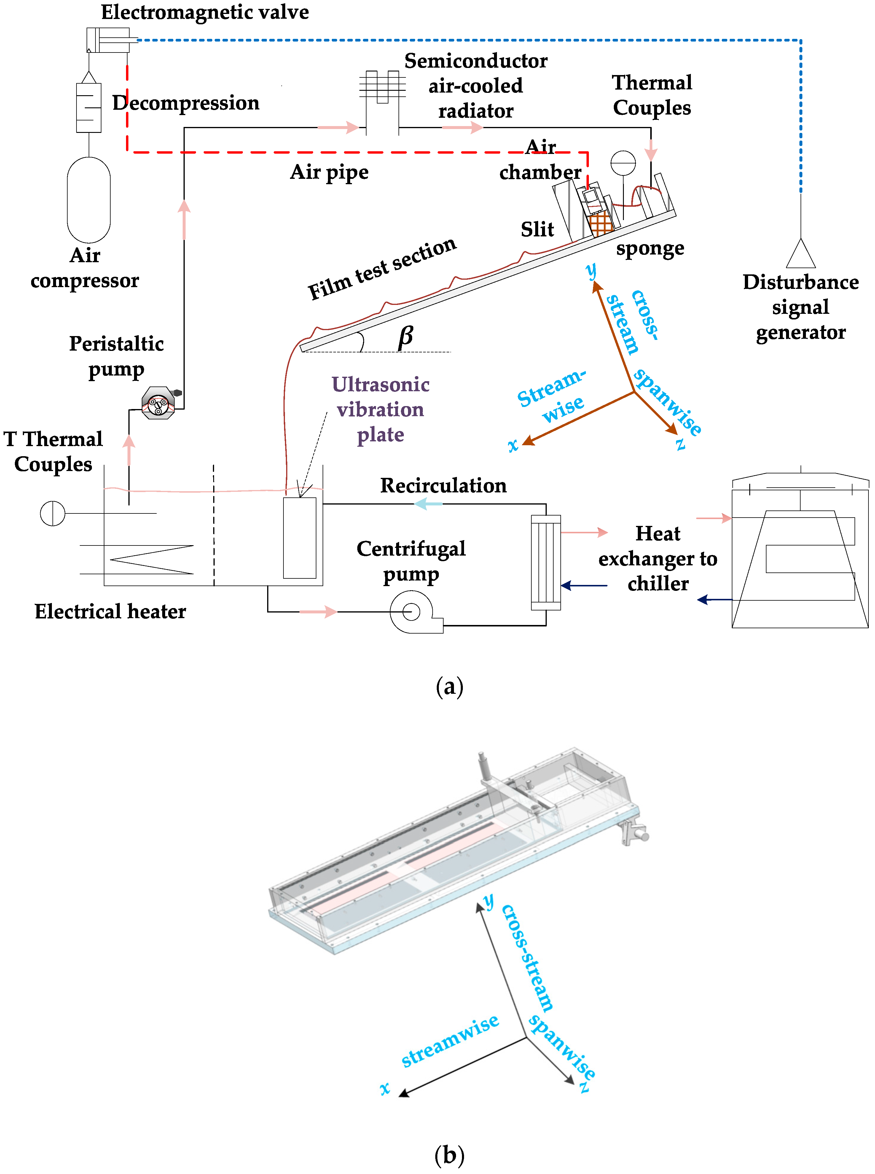
The PMMA box contains a flow distribution sector, an adjustable slit and film region. Inside the flow distribution section, three chambers are partitioned. The first chamber is set to overflow. As for the second and the third chamber, between which the separation plate is not glued to the substrate. The third chamber is tightly stuffed with sponge and covered with a thick hollow plate, which worked as air chamber allowing for perturbing the entrance flow rate at frequency f by small pressure variations as shown in Figure 1.

Finally, flow is dispensed evenly along the spanwise direction of the glass plate with a constant flow. A narrow and adjustable slit is installed at the exit of the distribution box, which could be adjusted by the micrometer heads, the slit gate has a thickness of 30 mm and width the same as the plate’s width. The thickness of the slit is set to 0.5 mm and examined by wedge plug ruler before the experiments. The effective film region is about 500 mm × 200 mm, and the measurements in this article were taken at 350 mm downstream of the slit and center in the spanwise direction.

2.2. Flow Loop

A schematic presentation of the flow loop configuration is given in Figure 1. The loop consists of the inclined film test section, a closed-loop circulating fluid from stainless steel tank via a peristaltic pump to the film test section, at the end of test section, liquid is collected and channeled back in the tank.

Type T thermal couples are installed in the loop to monitor the liquid temperature during the experiments. There are two temperature probe positions in the loop, one is inside the tank, the other is at the distribution chamber of film test section. Temperature signals are collected by DAQami software via MCC-TC modules (MCC, National Instruments: Norton, MA, USA).

Film test section, together with PIV system, are set up on an optical table, which can provide additional vibrating/shocking absorbing ability and a reference plane for the experiment. A stainless-steel water tank, located next to the optical table’s long side, served as a reservoir for fluid circulating via the loop. Next to the tank outlet, there is a recirculating loop to maintain the doped particles from sedimentation. An electrical heater is installed in the tank and a heat exchanger, which connects to an industrial chiller on its shell side in the recirculating loop, works together to keep the liquid temperature constant at T = 20 ± 0.5 °C. Hence, the recirculating loop could also provide additional heat removal capacity besides dissipation via heat conduction and convection.

Liquid in the test section is pumped by a peristaltic pump. Peristaltic pump could provide constantly pulsated flow rates, which might be too small to be adjusted precisely by normal centrifugal pump even with the aid of frequency variable or bypass valves. The precision of liquid flow rate provided by the peristaltic pump was calibrated with a graduated measuring glass cylinder and a stop watch. However, to isolate pump and pipes’ vibration from influencing the test section, the pump and related tubes are guided with an additional rack which is not attached to the optical table.

2.3. PIV/PLIF System

To capture images of film cross section (x-y plane in Figure 1) with relatively large spanwise (z in Figure 1) width, PIV/PLIF system consisting of customized illumination and image acquisition is utilized to fulfill the measurement task.

Usually, micro-PIV [22] (also μ-PIV) is characterized with high optical magnification, low depth of field, and volume illumination. It is also common practice that in micro-PIV applications, optical axis of the scope is perpendicular to the object plane and imaged volume controlled by microscope’s depth of field rather than planar illumination in traditional PIV. While the PIV/PLIF practice presented in this article has a high optical magnification (5×), it has large depth of field and thin laser sheet illumination determining image plane for film flowing on an inclined plate. Image access would be limited from below the glass plate. Hence, optical axis of the scope is no longer perpendicular to the image plane.

The laser source in the system is a continuous wave (CW) Nd:YAG 532-nm laser, which could provide 6 W illumination in a given region. The beam laser is shaped via a plano-concave cylindrical lens (f = −25.4 mm) diverging the laser into a planer sheet and a plano-convex cylindrical lens (f = 100 mm) reducing the beam waist diameter, which could effectively lower the ambiguity due to illumination thickness being comparable with the film thickness when the camera lens is inclined [23]. The final illumination is a light sheet with thickness under 100 μm in vicinity of lens focus, and the light-sheet thickness is approximately constant over the entire region of interest.

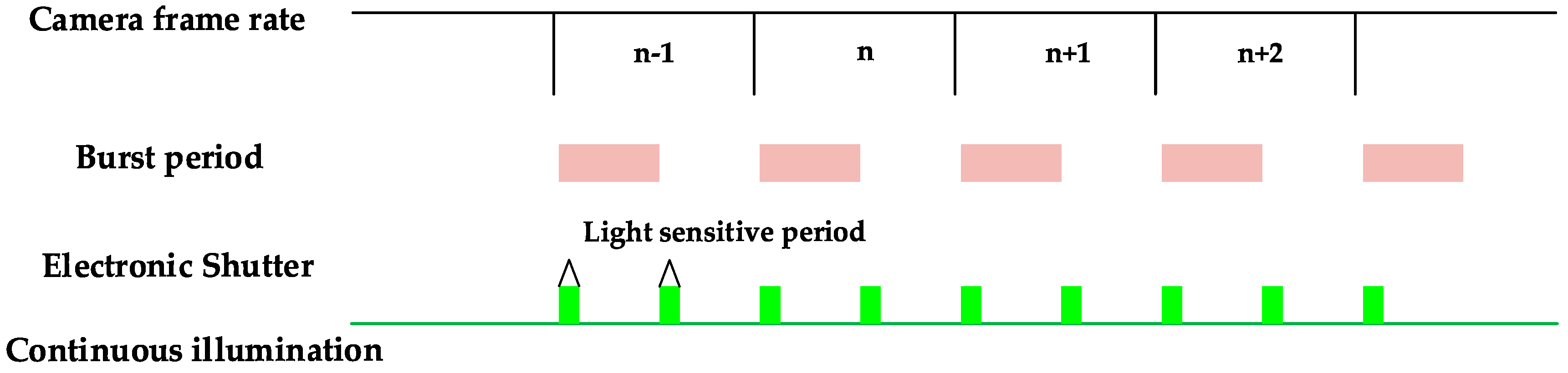
Illuminated film cross section is imaged with a high-speed camera (Vision Research, model Phantom V711, Wayne, NJ, USA) through an ultra-macro lens (Anhui Changgeng Optics Technology, LAOWA ULTRA MACRO lens, Hefei, Anhui, China). The lens can provide 2.5–5 fold optical magnification, 40–45 mm working distance, and relatively large depth of field, which ensure the whole film region could be imaged even if the focused plane is not coincided with the desired film cross-section. The high-speed camera is set to work in burst acquisition mode with 1280 × 400 pixels. Recording with burst acquisition mode and continuous illumination realized the dual frame/singe exposure PIV by capturing information on complementary metal-oxide-semiconductor (CMOS) as separate images in each light sensitive period during one frame instead of one image for one frame period, which allows flexible parameters adjustment at various flow conditions. A timing diagram is given in Figure 2 to illustrate how PIV recording based on the burst acquisition mode. Detailed information about burst acquisition mode can be found from Vision Research Customer Community provided by Vision Research.

Table 1. PIV parameters in film measurements.

Parameter	Value
Maximum velocity	About 0.3 m/s
Field of view	5.12 mm × 1.6 mm
Working distance	About 42 mm
Recording method	Double frame/single exposure
Recording medium	CMOS 1280 × 400 pixels, 20 × 20 μm per pixel
Illumination	CW Nd:YAG laser at 532 nm
PIV record parameters	2000 Hz, 70–350 us, according to one-quarter rule [24]
Seeding material	Titanium dioxide, diameter 0.5 μm, 4.26 g/cm3

briefly summarizes the relevant parameters of PIV in the experiment for a quick review.

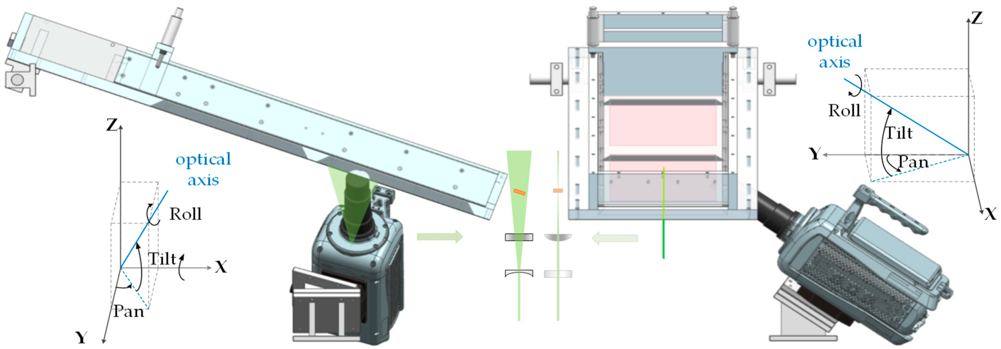
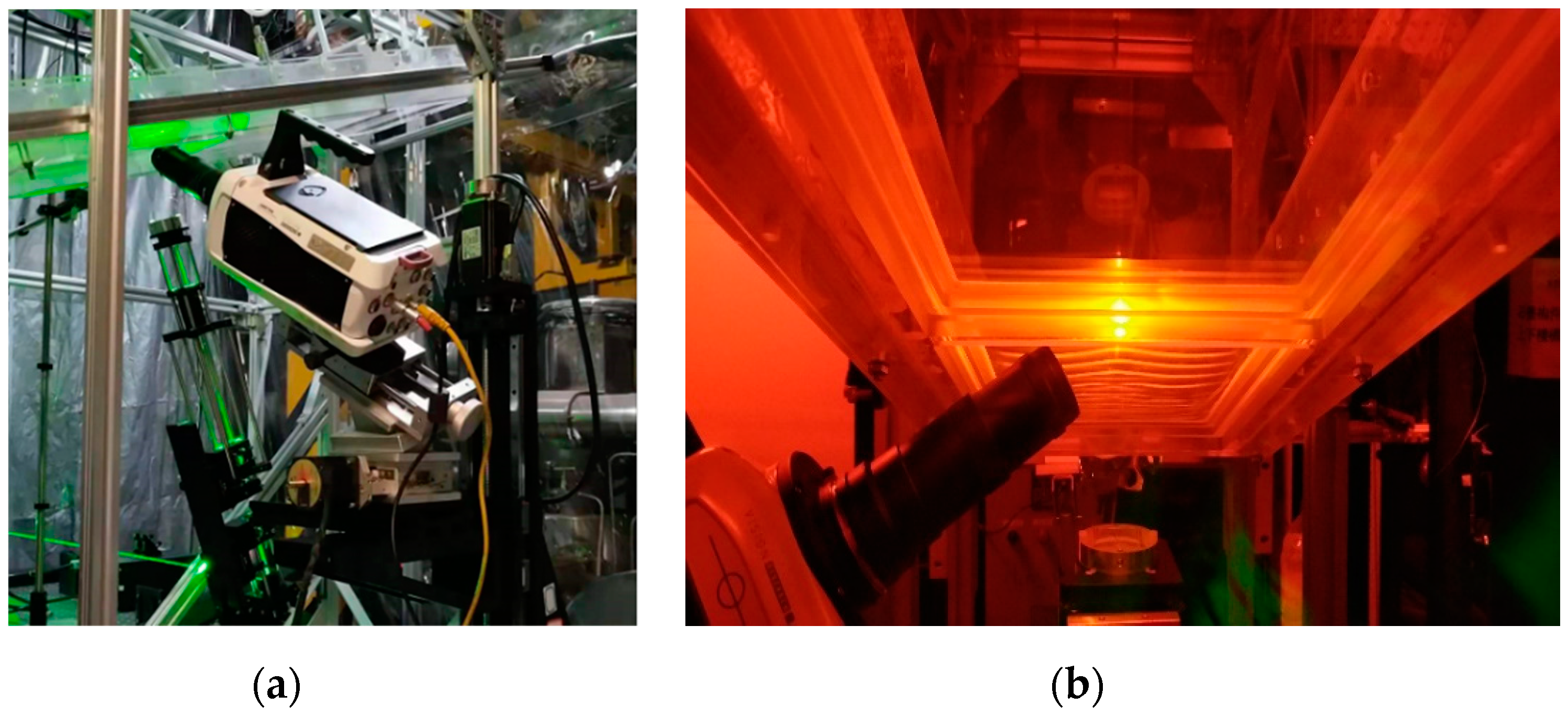
Camera installation is given in Figure 3 and Figure 4. Camera is mounted on two-axis goniometers, which are mounted on three-dimensional positioning stages. Two axis goniometers allow the camera and lens to roll with the inclination of the film, guarantee the imaged film bottom edge to be parallel to the camera sensor edge, and allow the tilt adjustment of the lens and camera to be properly placed below the glass plate. Here the tilt angle and roll angle are set to 35° and 20° (pan angle 0°).

For PIV, adequate particles are also an essential aspect to assure the fidelity of velocity measurement as PIV techniques determine velocity of tracer particles for the velocity of the fluid. The seeding particles used was 2 μm titanium dioxide particles. Fluid mechanical properties’ assessment of particles are provided by Dietze [7]. Based on the Basset–Boussinesq–Oseen (BBO) equation, the particle size can also guarantee good light scattering ability.

Besides particles, the fluids in the experiment are also doped with florescent dye (Rhodamine 6G). Additional fluorophore could radiate florescence photon of longer wavelength after excitation. For PIV/PLIF image recording, no filter was placed in front of the lens, both particle scattered light and florescence were recorded, which could distinct the liquid film from air or glass plate.

2.4. Film Experiment Conditions

In the experiments presented, the working fluids include deionized water and aqueous glycerol water (deionized water) solution (glycerol concentration 45% by volume). Properties of the working fluids are given in

Table 2. Working fluid property.

Working Fluid	ρ kg/m3	μ kg/(m·s)	σ N/m	Ka
Deionized water	0.998 × 103	10.06 × 10−4	72.75 × 10−3	4831.24
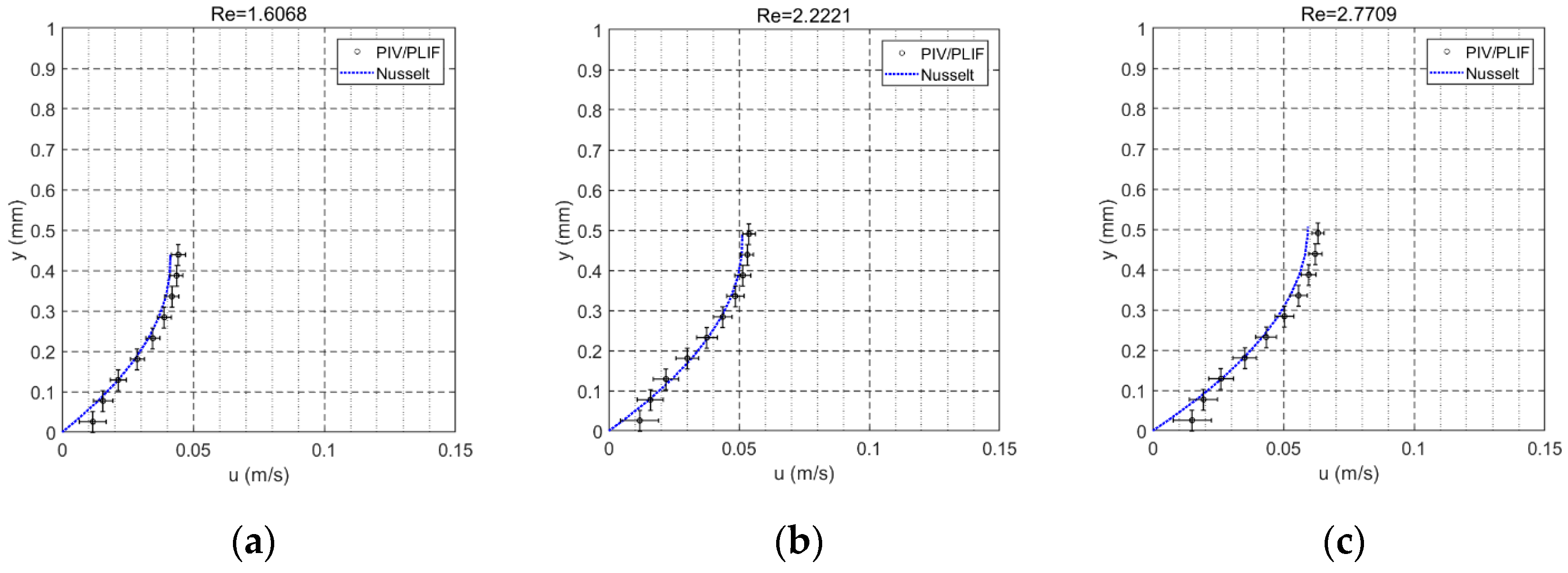
Glycerol water solution	1.120 × 103	81.03 × 10−4	65.4 × 10−3	278.83

below. The glycerol water solution is mainly used to validate the PIV method with Nusselt’s theory at a relatively low Reynold number.

With all the properties, the dimensionless groups are determined with the following equations. Reynold number:

$$Re=\frac{Q/W}{{\vartheta }_l},$$

(1)

where $Q$ represents the volume flow rate, $W$ denotes the film width, and ${\vartheta }_l$ is the kinematic viscosity of the working fluid.

Kapitza number:

$$Ka=\frac{{\sigma }_l}{{\rho }_l{\vartheta }_l{}^{4/3}{\left(sin\left(\beta \right)g\right)}^{1/3}},$$

(2)

where the ${\sigma }_l$ stands for surface tension of working liquid, ${\rho }_l$ is the density of working fluid, and g represents the gravitational acceleration.

Different experiment cases are listed in

Table 3. Experimental cases.

Name	Fluid	Re	Ka	f
Case 1	Water	80	4831.24	0 hz
Case 2	Water	50.3	4831.24	0 hz
Case 3	Glycerol	1.61	278.83	0 hz
Case 4	Glycerol	2.22	278.83	0 hz
Case 5	Glycerol	2.77	278.83	0 hz

, including glycerol water film cases for method validation and water film cases.

3. Experimental Methodology

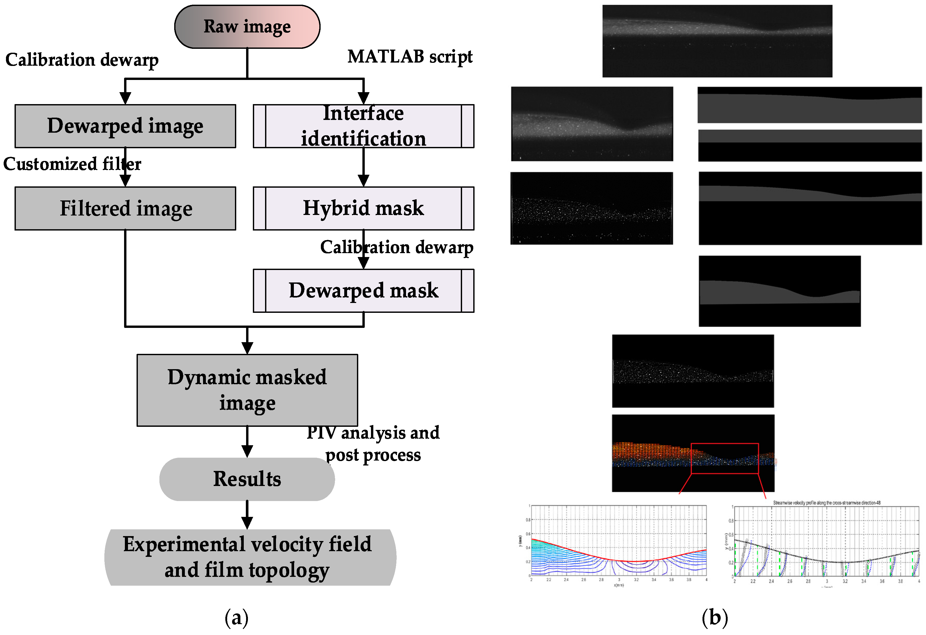
In PIV/PLIF experiments, unusual image acquisition can import image distortions and images have to be calibrated prior to PIV analysis. Hence, a series of image process procedures are adopted to correct the distortion and calibrate the images. Working fluids used in the experiment are mixed with both Rhodamine 6G dye and titanium dioxide particles. The PIV/PLIF image acquisition system is only equipped with one camera, making it unrealistic to acquire PLIF and PIV images separately. MATLAB scripts are used to process florescence information, forming dynamic masks to mask out a non-liquid zone. Florescence can indicate the fluid domain and the contrast of particle images against background can be decreased. Hence, a customized filter is used to enhance the particle images. After liquid zone in film recovered with MATLAB scripts and dynamic masking, advanced digital interrogation techniques are applied to enhance PIV correlation signal for evaluation of the PIV/PLIF images, data post process are also in use to minimize the random error. A schematic illustration of the PIV/PLIF process procedures and an example of the image process are displayed in Figure 5.

3.1. Image Pre-Processing: Image Calibration and Dewarp

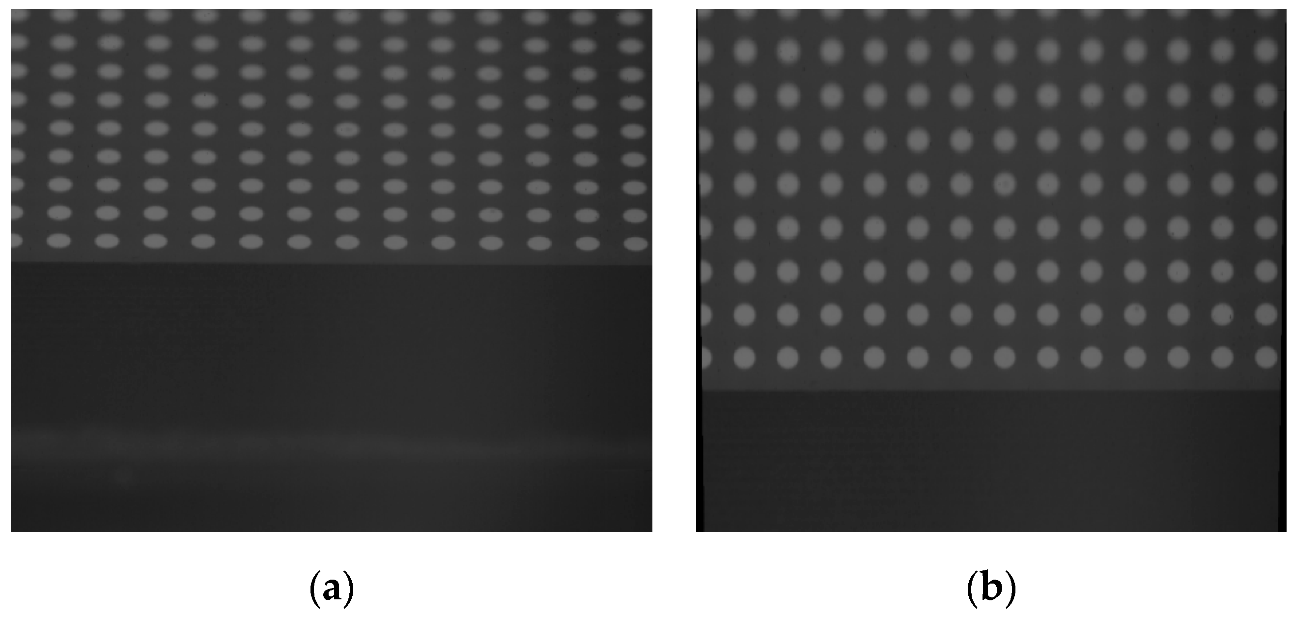
Recorded images are distorted. Implementation of image correction and calibration are essential before further analysis. The calibration target is a customized dotted array, bottom of the glass substrate is precise cut and milled to ensure minimum blanked area without damaging the dots. In calibration, a PMMA cuboid is used as a dam building up working fluid to immerse enough target and to ensure stable illumination. Calibration target image acquisition is in the same as PIV/PLIF recording, while enough large target was captured to cover all possible film regions.

Image distortion correction is accomplished with DynamicStudio 6.4 (Dantecs Dynamics: 16–18 Tonsbakken, DK-2740 Skovlunde, Denmark) by multi-camera calibration methods with a manual calibration target. After the calibration, distorted images are resampled with the calibration. Figure 6 gives the original image of the immersed target, and corrected target. However, there is some change in image size (pixels) after image de-warp, and some unnecessary portions of the image, which contain non-image information, can be imported.

3.2. Film Interface Identification

As aforementioned, working fluids used in the experiment are mixed with both florescent dye and titanium dioxide particles. The optical system in this research is only equipped with one camera, making it unrealistic to acquire florescence and particle images separately. Particle images in non-liquid zones could bring about an obscure flow field. It is indispensable to identify the interfaces of liquid film prior to further the process.

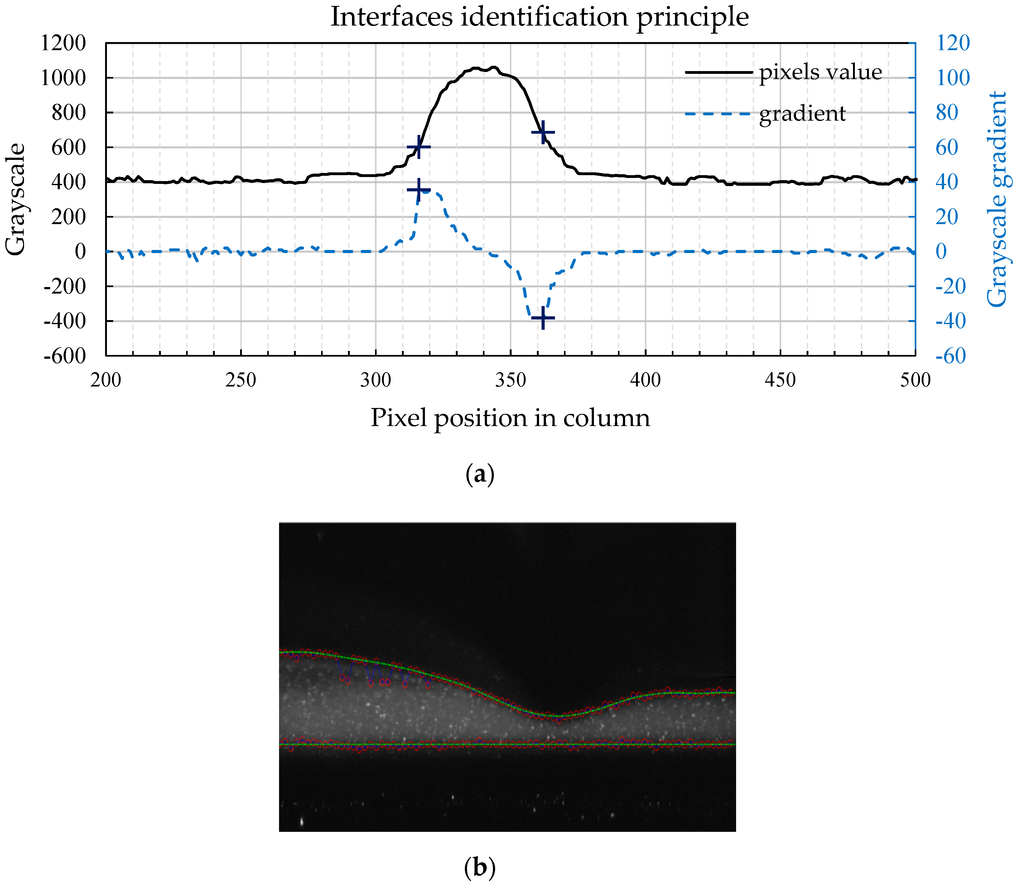
This interface identification method is accomplished with the convenience of MATLAB link in DynamicStudio. MATLAB link transfers data from DynamicStudio database to MATLAB’s workspace, allowing data analysis performed using MATLAB scripts. Afterwards, results can be transferred back to the DynamicStudio database for further processing. In MATLAB scripts, raw images are filtered with a median filter to remove peaks of particle images avoiding influence on background, the 2D filter has a width of more than twice of the particle image’s diameter in pixels (10 pixels as filter window size), separating the particle information from the fluorescence. Then averaged pixel grayscale profile of several columns are analyzed.

Figure 7 illustrates the typical grayscale profile in column direction and the interfaces are determined by the maxima and minima of pixel grayscale gradient. Derived liquid gas interface is further smoothed and fitted to a piecewise 5th degree polynomial based on segments divided by the inflection points [6], a linear function for the liquid glass interface. To be specific, the liquid–air interface and liquid–solid interface are acquired separately. Liquid–gas interface determined for every image pairs in the transient film flow situation and liquid glass interface determined with the averaged image pair of the whole set of image pairs. The image pixels above the liquid–gas interface and below the liquid–glass interface are masked out. Finally, masked images overlay into a hybrid mask, and hybrid dynamic masks are de-warped with the resample grid built in the calibration process.

3.3. PIV/PLIF Process and Data Post Process

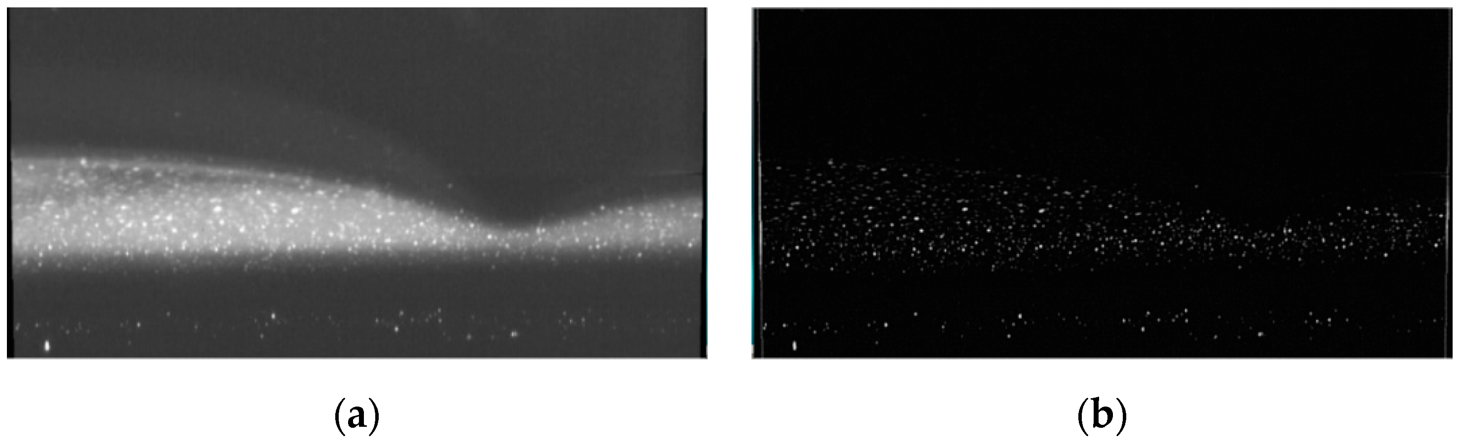
In the PIV process, dewarped images are filtered with a 5 × 5 custom filter kernel (an embedded filter kernel in DynamicStudio, DOG0305) with the means of a custom filter in the image process library to enhance the contrast of particle signal and background, and in this way the fluorescent background is removed. The effects of images are shown in Figure 8.

The PIV evaluation method applied here is adaptive PIV provided by DynamicStudio. The adaptive PIV method is an automatic and adaptive method for calculating velocity vectors based on particle image pairs. The method can iteratively adjust the size, shape, and location of the individual interrogation areas (IA) in order to adapt to local seeding densities and flow velocities and gradients. Hence, adaptive PIV enables better velocity measurement fidelity where the velocity gradient was strong [25,26].

In application, the adaptive PIV schemes parameters are maximum IA size: 64 × 32, minimum IA size: 32 × 16; and grid step size: 8 × 4. The non-equal interrogation grid step size takes film flow characteristics in consideration, where streamwise velocity u (corresponding to horizontal width) is predominant.

To prevent outliers from disturbing the adaptive iterations and the velocity results, validation is done by applying peak validation and universal outlier detection [27]. Peak height validation requires a minimum of 0.15 for correlation peaks and 4 for signal to noise (S/N) ratio. Parameters of universal outlier detection are of a neighborhood size at 5 × 3, minimum normalization 0.1, and acceptance limit 2.0. What’s more, results are further validated with a moving average validation (5 × 3 area with acceptance factor 0.1 and iteration 3) and smoothed with an average filter (5 × 3) to reduce the random noise.

3.4. PIV-Based Pressure Measurement

Deriving instantaneous pressure from flow velocity field data from PIV, based on the governing equations, is a novel non-intrusive diagnostic methodology. The feasibility of PIV-based pressure measurement has been demonstrated abundantly over recent years, notably for low speed and two-dimensional flow [28].

After PIV velocity results are obtained, pressure field of film flow are derived based on the velocity field. The approach taken here is the Poisson equation for computing the pressure. The principle of Poisson equation and its numerical implementation for the film pressure field are briefly given in the following:

Poisson equation is obtained from taking divergence of incompressible Navier-Stokes equations, which under incompressible assumption leads to Equation (4)

$$\nabla \mathrm{p}=\left(-\mathsf{\rho }\frac{\partial u}{\partial \mathrm{t}}-\mathsf{\rho }\left(u·\nabla \right)u+\mu {\nabla }^{2}u\right)$$

(3)

$${\nabla }^2\mathrm{p}=\nabla ·\left(-\mathsf{\rho }\frac{\partial u}{\partial \mathrm{t}}-\mathsf{\rho }\left(u·\nabla \right)u+\mu {\nabla }^{2}u\right)=-\mathsf{\rho }\nabla ·\left(u·\nabla \right)u$$

(4)

Even though there are no time derivatives in the final form of Equation (4), it is still applicable to transient conditions, because the time-dependent information is prescribed in boundary conditions. Expansion of Equation (4) under the condition of 2D incompressible unsteady flow, the Poisson equation for 2D flow reads:

$$\frac{{\partial }^2\mathrm{p}}{\partial {\mathrm{x}}^2}+\frac{{\partial }^2\mathrm{p}}{\partial {\mathrm{y}}^2}=-\mathsf{\rho }\left\{{\left(\frac{\partial \mathrm{u}}{\partial \mathrm{x}}\right)}^2+2\frac{\partial \mathrm{u}}{\partial \mathrm{y}}\frac{\partial \mathrm{v}}{\partial \mathrm{x}}+{\left(\frac{\partial \mathrm{v}}{\partial \mathrm{y}}\right)}^2\right\}$$

(5)

Numerical implementation of Poisson equation is through the following equations, the corresponding boundary condition include Dirichlet condition for liquid gas interfaces and Neumann condition for the rest boundaries. The pressure distribution for Dirichlet condition is determined by surface tension [29] as Equation (8) and pressure gradient for Neumann condition is determined with Equation (3). With proper boundary condition and acceleration field, the pressure can be derived after iterations.

$$q=-\mathsf{\rho }\left\{{\left(\frac{\partial \mathrm{u}}{\partial \mathrm{x}}\right)}^2+2\frac{\partial \mathrm{u}}{\partial \mathrm{y}}\frac{\partial \mathrm{v}}{\partial \mathrm{x}}+{\left(\frac{\partial \mathrm{v}}{\partial \mathrm{y}}\right)}^2\right\}$$

(6)

$$\frac{{\mathrm{p}}_{\mathrm{i}+1,\mathrm{j}}-2{\mathrm{p}}_{\mathrm{i},\mathrm{j}}+{\mathrm{p}}_{\mathrm{i}-1,\mathrm{j}}}{{\left(·\mathrm{x}\right)}^2}+\frac{{\mathrm{p}}_{\mathrm{i},\mathrm{j}+1}-2{\mathrm{p}}_{\mathrm{i},\mathrm{j}}+{\mathrm{p}}_{\mathrm{i},\mathrm{j}-1}}{{\left(·\mathrm{y}\right)}^2}={\mathrm{q}}_{\mathrm{i},\mathrm{j}}$$

(7)

$${\mathrm{p}}_{\mathsf{\delta }}=-\mathsf{\sigma }\frac{{\mathsf{\delta }}_{\mathrm{xx}}}{{\left(1+{\mathsf{\delta }}_{\mathrm{x}}{}^2\right)}^{3/2}}$$

(8)

4. Discussion Results Discussion

4.1. Method Validation

When Re < Rec (5/4cot(β), about 3.4 for β = 20°) film flow falling on an inclined plate is developed on laminar flow submits to the Nusselt flat film solution [1,30], after Re>Rec, flow instability commences, and streamwise velocity profile can deviate from the semi-parabolic profile. Hence, PIV/PLIF measurement is validated by comparing the experimental results of steady smooth film flow (Case 3–5) with the Nusselt flat film solution. Figure 9 illustrates comparisons between the experimental velocity profile and corresponding theoretical profiles based on Equations (9) and (10). For PIV/PILF results, horizontal error bars illustrate standard deviation of measurement data, vertical error bars are given by half of cross-stream resolution’s spatial dimension.

$$u=\frac{\sin \left(\beta \right)g}{{\vartheta }_l}y\left(\delta -\frac{y}{2}\right),$$

(9)

$$\delta ={\left(\frac{3Re{\vartheta }_l{}^2}{\sin \left(\beta \right)g}\right)}^{\frac{1}{3}},$$

(10)

Comparison shows good agreement between the two data sets, despite the velocity in near wall region (0–0.1 mm) is biased for average effect where strong velocity gradient near wall exists [31,32].

Comparing the analytical film thickness, the PLIF derived film thickness matches well with the theoretical prediction, and the error is in the range of the cross stream spatial resolution’s dimension. The general conclusion can be draw that the PIV/PLIF experimental results of film flow matched well with the Nusselt’s theoretical prediction for both film thickness and velocity profile.

The above validations are mainly based on flat film. To directly further check the validity of instantaneous wavy film velocity field and transient topology, we resorts to continuity equation in integral form [33]. The integral continuity Equation (11) is derived from continuity with kinematic boundary condition at free surface, hence high fidelity velocity and topology is required to acquire a satisfying replica from an experimental outcome. Continuity validation results of Case 1 and Case 2 are presented in Figure 10. The negative value of experimental thickness time derivative agrees well with the flow rate stream-wise derivative, assuring the validity and accuracy of the experimental techniques.

$$\frac{\partial \mathrm{h}}{\partial \mathrm{t}}+\frac{\partial \mathrm{q}}{\partial \mathrm{x}}=0,$$

(11)

4.2. Capillary Wave Dynamics

Results and discussion mainly focus on solitary waves, especially capillary waves. Without any classification for solitary wave regions, further elucidation may seem rather confusing. Therefore, Figure 11 summarizes the typical terminology for solitary waves used hereinafter in this article.

Capillary waves and flow reversal related results in the literature are mainly given with spatial distribution like snapshots of velocity distribution at a certain time. With high-performance experiment facilities, we are able to provide results in both spatial mode and temporal mode for better elucidation of the traveling wave. Figure 11 and Figure 12 are listed here as elucidation of traveling wave in spatial mode and temporal mode. The same case may seem to be inversed in the x axis. Comparison between spatial mode and temporal mode could make the elaboration of capillary wave dynamics more explicit and intuitive.

For better elucidation, different image results are rearranged in the order of their streamwise position from upstream to downstream as shown in Figure 11. In the velocity profile chart, velocity is given in the laboratory frame, the green dashed line represents streamwise probe positions of velocity profile, and reference y axis indicates zero value for the velocity magnitude. The black circle dots represent PIV/PLIF results, blue dotted lines are parabolic profiles calculated from Nusselt’s theory Equations (9) and (10) and local film thickness, both experimental velocity and predicted velocity are scaled with the same factor to fit streamwise spatial dimension. The number in the velocity profile chart title are time coordinates for cross reference with other data of the same case. Careful examination of Figure 13 and Figure 14 show that the conclusions that could be drawn are:

• Evident flow reversal in the first and second capillary troughs are observed, negative streamwise velocities in laboratory frame of reference. In regions of the first and second capillary troughs, open shaped vortices, evidences flow reversal happened, which is consistent with results of Dietze [6,7], despite different fluid (DSMO), film plate (vertical tube), and controlled disturbance. There are no vortices in the third vortices, only velocity vectors gradually departure from the plate and re-approach the plate afterwards.
• Compared to the measured instantaneous streamwise velocity profile in the regions of the front of the main hump, Nusselt theory significantly overestimates the streamwise velocity. The maximum value exceeds the experimental results by about 100%. In a qualitative manner, streamwise velocity profile under capillary wave peak appears closer to the parabolic form. While the streamwise velocity profile in capillary wave troughs deviates significantly from the parabolic form.

4.3. Flow Reversal Mechanism

The onset of flow reversal is symbolled with a vanishing local flow rate (averaged streamwise velocity equals zero), a surface velocity of zero or sign change of local shear stress [8,19,20]. Criterion for flow reversal in this article is zero value of averaged streamwise velocity, once it is negative, flow reversal would be considered to have happened.

The mechanism in the literature for flow reversal in capillary waves troughs were primarily illustrated with pressure or pressure gradient in a spatial mode. For example, Dietze [6,8] confirmed that it was the pressure gradient inside the liquid film that led to flow reversal, to be specific, streamwise pressure gradient to gravity ratio was used to symbolize the dynamic of flow reversal.

According to canonical pressure distribution given in Figure 14(a2), which shows similar distribution with numerical works [21] considering its surface curvature, pressure gradient in the region in the front of the main hump (from the peak of main hump to the first capillary minimum) is negative, positive pressure gradient in region back of the first capillary wave (from the first capillary minimum to the first capillary maximum), and negative pressure gradient in the region at the front of the first capillary wave. Pressure gradient in the rest regions of capillary waves could be deduced similarly.

For falling liquid film on an inclined plate, the dominant factor determining the pressure field in film is surface tension. The solitary wave remains unchanged in the observed range as the wave propagates, the pressure field, and pressure gradient would move forward with traveling waves. With typical pressure field and pressure gradient distribution in solitary wave, elaboration of flow reversal mechanism in a spatial mode might be misleading: based on pressure gradient spatial distribution, liquid under front of main hump will be accelerated and afterwards decelerated in the back of the first capillary wave crest. In this way, negative averaged streamwise velocity would not exist, nor did streamwise velocity agreed with actual flow field in capillary wave regions.

With pressure derived from high sample rate transient velocity field, an intuitive way to reproduce the flow reversal dynamics in temporal mode would be feasible. Probe velocity, pressure, pressure gradient at x = 1.291 mm, correlating time traces are presented in Figure 15. The pressure gradient is presented by ratio (Ψ in Figure 15) of streamwise pressure force per unit volume to streamwise gravitational force per unit volume for better analysis of composition forces in liquid film.

$$\mathsf{\Psi }=\frac{\partial \mathrm{p}}{\partial \mathrm{x}}/{\left(\rho g\right)}_x,$$

(12)

To review, for falling liquid film flow: (1) pressure field is primary determined by surface topology, (2) solitary waves travel unchanged in the imaged range, (3) wave velocity is higher than the liquid velocity in capillary wave regions. It could be interpreted that: in temporal mode, the front of waves passes through certain streamwise positions and the back of waves arrive then; the second capillary wave passes prior to the first capillary waves.

For data in Figure 15, from t = 48 to t = 58, the second capillary wave minimum to the first capillary maximum (front of the first capillary wave crest region) flows through x = 1.291 mm, the liquid experiences a negative flow pressure gradient. During this period, the force ratio Ψ was less than 1. Hence, the composition of pressure and gravity for liquid element is small in the downstream and large in the upstream, liquid here would be accelerated. From t = 59 to t = 68, the first capillary maximum to the first capillary minimum (back of the first capillary wave crest region) flows through x = 1.291 mm, according to the time traces of force ratio Ψ, it can be confirmed that the liquid elements here experience positive pressure gradient, and the ratio Ψ is greater than 1 during this period, meaning that composition of pressure and gravity for liquid element is large in the downstream and small in the upstream, and the liquid can be decelerated. Similar acceleration can happen for the front of main hump region as the front of the first capillary wave crest region.

Taking into account the third second and first capillary wave for comparison, maximum averaged streamwise velocity at wave maximum is comparative, while the force ratio gradually decreases, the absolute value of averaged streamwise velocity at wave minimum increases, and only in the first and second capillary trough does the flow reversal phenomena exist. The correlating results could be interpreted as the following: only when the capillary wave liquid film curvature changes are strong enough to produce a considerable positive pressure gradient, and the liquid deceleration would be enough to reduce the liquid velocity to negative values, as the dynamics given in Figure 15. Similar results could also be concluded from Case 2 according to Figure 16.

By analyzing time traces of experimental results, the mechanism of flow reversal phenomenon in the capillary wave trough is given in the temporal mode, the key region for deceleration, which promotes the onset of flow reversal is the back of capillary wave crests, instead of the capillary troughs or front of main hump.

Previous solitary wave dynamics-related studies have reported maximum wave height stagnates when increasing the Reynolds number above a critical value, and attained a global minimum of the film thickness for all considered cases [18,35]. To compensate the increasing curvature at larger Reynold numbers, the number of capillary waves will increase and capillary wave length decrease [36]. Velocity of the solitary wave and capillary wave is related to the maximum wave height. Based on the dynamics of flow reversal given in temporal mode and solitary wave dynamics, we might provide a conjecture for flow reversal upper threshold: The deceleration would gradually saturate with curvature, while deceleration duration would be decreasing as the capillary wave length decreases with increasing inertia. Eventually, the deceleration will not decrease the streamwise velocity to negative values and flow reversal will cease to onset.

5. Conclusions

This work presents a set of special designed experimental facilities for falling liquid film with a large Ka number. A laser diagnosis technique combining PIV and PLIF with only one camera was used to measure film internal velocity field and film topology. Satisfactory agreement between of the experimental velocity profile and film thickness with the Nusselt flat-film solution predictions was achieved and meanwhile the validity and accuracy of the PIV/PLIF experimental methodology was further verified with a good match of the continuity equation based on transient velocity and film topology.

Film velocity fields and film topology of capillary waves are experimentally measured, in which the occurrence of negative streamwise velocity in the laboratory reference frame suggests that flow reversal appears at capillary wave troughs. In addition, the measured streamwise velocity profiles show that it is deviated from a common semi-parabolic velocity profile of film flow.

Liquid flow can experience acceleration in front of the main hump and then suffer from deceleration at the back of the first capillary wave crest according to canonical pressure spatial distribution, which is inconsistent with flow reversal. Flow reversal mechanism at the capillary wave is revealed from temporal evolution of streamwise velocity and pressure gradient: For a fixed point in streamwise direction, downstream tide and upstream counterpart pass its location in sequence; hence, positive pressure gradient at the back of the first capillary wave crest can lead to fluid element deceleration and eventually trigger an onset of flow reversal at the first capillary trough. Conjecture for upper threshold mechanism of flow reversal is speculated to be based on the flow reversal dynamics in the temporal mode, which might come from gradually saturated deceleration and shorter capillary waves duration as the reduced Reynold number is high enough.

References

1. Kalliadasis, S.; Ruyer-Quil, C.; Scheid, B.; Velarde, M.G. Falling Liquid Films, 1st ed.; Springer: London, UK, 2012. [Google Scholar]
2. Pereira, O.; Rodríguez, A.; Barreiro, J.; Fernández-Abia, A.I.; de Lacalle, L.N.L. Nozzle design for combined use of MQL and cryogenic gas in machining. Int. J. Precis. Eng. Manuf.-Green Technol. 2017, 4, 87–95. [Google Scholar] [CrossRef]
3. Ter Haar, D. (Ed.) Wave flow of thin layers of a viscous fluid. In Collected Papers of P.L. Kapitza; Elsevier: Oxford, UK, 1965; pp. 662–709. [Google Scholar]
4. Adomeit, P.; Renz, U. Hydrodynamics of three-dimensional waves in laminar falling films. Int. J. Multiph. Flow 2000, 26, 1183–1208. [Google Scholar] [CrossRef]
5. Alekseenko, S.V.; Antipin, V.A.; Bobylev, A.V.; Markovich, D.M. Application of PIV to velocity measurements in a liquid film flowing down an inclined cylinder. Exp. Fluids 2007, 43, 197–207. [Google Scholar] [CrossRef]
6. Dietze, G.F.; Kneer, R. Flow separation in falling liquid films. Front. Heat Mass Transf. 2011, 2, 033001. [Google Scholar] [CrossRef] [Green Version]
7. Dietze, G.F.; Alsibai, F.; Kneer, R. Experimental study of flow separation in laminar falling liquid films. J. Fluid Mech. 2009, 637, 73–104. [Google Scholar] [CrossRef]
8. Dietze, G.F.; Leefken, A.; Kneer, R. Investigation of the backflow phenomenon in falling liquid films. J. Fluid Mech. 2008, 595, 435–459. [Google Scholar] [CrossRef]
9. Ashwood, A.C.; Hogen, S.J.V.; Rodarte, M.A.; Kopplin, C.R.; Rodríguez, D.J.; Hurlburt, E.T.; Shedd, T.A. A multiphase, micro-scale PIV measurement technique for liquid film velocity measurements in annular two-phase flow. Int. J. Multiph. Flow 2015, 68, 27–39. [Google Scholar] [CrossRef]
10. Charogiannis, A.; Markides, C.N. Spatiotemporally resolved heat transfer measurements in falling liquid-films by simultaneous application of planar laser-induced fluorescence (PLIF), particle tracking velocimetry (PTV) and infrared (IR) thermography. Exp. Therm. Fluid Sci. 2019, 107, 169–191. [Google Scholar] [CrossRef]
11. Charogiannis, A.; Denner, F.; Wachem, B.G.M.V.; Kalliadasis, S.; Markides, C.N. Detailed hydrodynamic characterization of harmonically excited falling-film flows: A combined experimental and computational study. Phys. Rev. Fluids 2017, 2, 014002. [Google Scholar] [CrossRef] [Green Version]
12. Charogiannis, A.; An, J.S.; Markides, C.N. A simultaneous planar laser-induced fluorescence, particle image velocimetry and particle tracking velocimetry technique for the investigation of thin liquid-film flows. Exp. Therm. Fluid Sci. 2015, 68, 516–536. [Google Scholar] [CrossRef] [Green Version]
13. Denner, F.; van Wachem, B.G.M. Numerical time-step restrictions as a result of capillary waves. J. Comput. Phys. 2015, 285, 24–40. [Google Scholar] [CrossRef] [Green Version]
14. Reck, D.; Aksel, N. Recirculation areas underneath solitary waves on gravity-driven film flows. Phys. Fluids 2015, 27, 3–28. [Google Scholar] [CrossRef]
15. Portalski, S. Eddy Formation in Film Flow Down a Vertical Plate. Ind. Eng. Chem. Fundam. 1964, 3, 49–53. [Google Scholar] [CrossRef]
16. Tihon, J.; Serifi, K.; Argyriadi, K.; Bontozoglou, V. Solitary waves on inclined films: Their characteristics and the effects on wall shear stress. Exp. Fluids 2006, 41, 79–89. [Google Scholar] [CrossRef]
17. Tihon, J.; Tovchigrechko, V.; Sobolík, V.; Wein, O. Electrodiffusion detection of the near-wall flow reversal in liquid films at the regime of solitary waves. J. Appl. Electrochem. 2003, 33, 577–587. [Google Scholar] [CrossRef]
18. Chakraborty, S.; Nguyen, P.K.; Ruyer-Quil, C.; Bontozoglou, V. Extreme solitary waves on falling liquid films. J. Fluid Mech. 2014, 745, 564–591. [Google Scholar] [CrossRef]
19. Rohlfs, W.; Pischke, P.; Scheid, B. Hydrodynamic waves in films flowing under an inclined plane. Phys. Rev. Fluids 2017, 2, 044003. [Google Scholar] [CrossRef]
20. Rohlfs, W.; Scheid, B. Phase diagram for the onset of circulating waves and flow reversal in inclined falling films. J. Fluid Mech. 2015, 763, 322–351. [Google Scholar] [CrossRef] [Green Version]
21. Denner, F.; Charogiannis, A.; Pradas, M.; Markides, C.N.; Wachem, B.G.M.V.; Kalliadasis, S. Solitary waves on falling liquid films in the inertia-dominated regime. J. Fluid Mech. 2018, 837, 491–519. [Google Scholar] [CrossRef] [Green Version]
22. Adrian, R.J. Twenty years of particle image velocimetry. Exp. Fluids 2005, 39, 159–169. [Google Scholar] [CrossRef]
23. Kähler, C.J.; Scholz, U.; Ortmanns, J. Wall-shear-stress and near-wall turbulence measurements up to single pixel resolution by means of long-distance micro-PIV. Exp. Fluids 2006, 41, 327–341. [Google Scholar] [CrossRef]
24. Raffel, M. Particle Image Velocimetry A Practical Guide, 3rd ed.; Springer International Publishing: Cham, Switzerland, 2018. [Google Scholar]
25. Theunissen, R.; Scarano, F.; Riethmuller, M. Spatially adaptive PIV interrogation based on data ensemble. Exp. Fluids 2010, 48, 875–887. [Google Scholar] [CrossRef]
26. Theunissen, R.; Scarano, F.; Riethmuller, M. On improvement of PIV image interrogation near stationary interfaces. Exp. Fluids 2008, 45, 557–572. [Google Scholar] [CrossRef] [Green Version]
27. Westerweel, J.; Scarano, F. Universal outlier detection for PIV data. Exp. Fluids 2005, 39, 1096–1100. [Google Scholar] [CrossRef]
28. Van Oudheusden, B.W. PIV-based pressure measurement. Meas. Sci. Technol. 2013, 24, 032001. [Google Scholar] [CrossRef]
29. Malamataris, N.A.; Vlachogiannis, M.; Bontozoglou, V. Solitary waves on inclined films: Flow structure and binary interactions. Phys. Fluids 2002, 14, 1082–1094. [Google Scholar] [CrossRef]
30. Liu, J.; Paul, J.D.; Gollub, J.P. Measurements of the primary instabilities of film flows. J. Fluid Mech. 1993, 250, 69–101. [Google Scholar] [CrossRef]
31. Kähler, C.J.; Scharnowski, S.; Cierpka, C. On the resolution limit of digital particle image velocimetry. Exp. Fluids 2012, 52, 1629–1639. [Google Scholar] [CrossRef] [Green Version]
32. Kähler, C.J.; Scharnowski, S.; Cierpka, C. On the uncertainty of digital PIV and PTV near walls. Exp. Fluids 2012, 52, 1641–1656. [Google Scholar] [CrossRef] [Green Version]
33. Ruyer-Quil, C.; Manneville, P. Improved modeling of flows down inclined planes. Eur. Phys. J. B-Condens. Matter Complex Syst. 2000, 15, 357–369. [Google Scholar] [CrossRef]
34. Wilko, R.; Manuel, R.; Benoit, S. WaveMaker: The three-dimensional wave simulation tool for falling liquid films. Softw. X 2018, 7, 211–216. [Google Scholar]
35. Denner, F.; Pradas, M.; Charogiannis, A.; Markides, C.N.; van Wachem, B.G.; Kalliadasis, S. Self-similarity of solitary waves on inertia-dominated falling liquid films. Phys. Rev. E 2016, 93, 033121. [Google Scholar] [CrossRef] [PubMed] [Green Version]
36. Dietze, G.F. On the Kapitza instability and the generation of capillary waves. J. Fluid Mech. 2016, 789, 368–401. [Google Scholar] [CrossRef]
Figure 1. (a) Schematic diagram of experiment flow and perturbation system, flow loop, and film test section. (b) Film test section. The italic letters x y z denotes the streamwise cross-stream and spanwise directions in the coordinate system of film.
Coatings 10 00599 g001
Figure 2. Timing diagram for PIV/PLIF recording based on burst acquisition mode, burst count = 2, both exposure images were stored for further process.
Coatings 10 00599 g002
Figure 3. Film test section and PIV/PLIF system, the high-speed camera is setup besides the test section as the figure illustrates. XYZ axis in this Figure are referred as the world coordinate system to give a proper description of the camera’s angular orientation. The green plane represents the laser sheet in the middle, light sheet optics using two cylindrical lenses are given for better illustration of the PIV/PLIF image acquisition.
Coatings 10 00599 g003
Figure 4. (a) Photograph of PIV/PLIF measurement in falling film experiment. (b) Photo taken with a high pass filter.
Coatings 10 00599 g004
Figure 5. (a) PIV/PLIF process procedures. (b) PIV/PLIF process example. Each of the procedures in (a) corresponds to an image outcome in (b). In (a) PIV portion are given in gray color and PLIF related process are given in pale pink color.
Coatings 10 00599 g005
Figure 6. (a) Original target image acquired in experiments, the distortion could be seen clearly with tilt of dot column and image. (b) Target image after calibration and dewarp, two edges of the image are filled with blank pixels during the de-warp process.
Coatings 10 00599 g006
Figure 7. (a) Interface identification principle, (b) Interface fit for liquid gas interface and liquid solid interface, the circle points are raw results and dash line represents the fitting curve. The image is adjusted with vertical scale enlarged for better display effect.
Coatings 10 00599 g007
Figure 8. (a) Dewarped image and (b) filtered image. In comparison, custom filter could be used to remove the fluorescence background and enhance particle signal contrast.
Coatings 10 00599 g008
Figure 9. Comparison of PIV/PLIF and analytical crosswise profile of the streamwise velocity component u for smooth water-glycerin film (Case 3–5, (a)–(c)). For PIV/PILF results, horizontal error bars illustrate standard deviation of measurement data, vertical error bars are given by half of cross-stream resolution’s spatial dimension.
Coatings 10 00599 g009
Figure 10. Continuity validation for instantaneous velocity dynamics and topology of Case 1 (a) and Case 2 (b). The time index in this figure title corresponds to time index of figures in Section 4.2.
Coatings 10 00599 g010aCoatings 10 00599 g010b
Figure 11. Regions in a single hump solitary wave: back of main hump, main hump, front of main hump, capillary waves, residual film substrate. For capillary ripples, in each capillary wave, the peak is assigned as capillary maximum, and the lowest in trough is assigned as capillary minimum. In streamwise direction, the capillary wave is assigned as the first, the second, and so on. In capillary waves, front and back would also be assigned in the same order as for the main hump. This picture is a snapshot of film thickness distribution taken from WaveMaker [34] simulation Case III for its typical solitary wave pattern, which serves as the example of travel waves in spatial mode. Reprinted with permission from [34] Copyright year Copyright owner’s name.
Coatings 10 00599 g011
Figure 12. Film thickness temporal evolution in a fixed streamwise position, data here is from the same case as in Figure 11. The thickness time traces are adopted here for illustration of travel waves in temporal mode.
Coatings 10 00599 g012
Figure 13. Capillary waves dynamics for Case 1. (a) Front of main hump. (b) First capillary wave trough and crest. (c) Second capillary wave trough and crest. (d) Third capillary wave trough and crest. In profile chart, green dashed lines give streamwise probe positions for velocity profile that also serve as reference y axis indicating zero value for velocity magnitude, the dark circle dots represent the measured results, blue dotted lines are the parabolic profile based on Nusselt’s theory and local film thickness, both experimental velocity and predicted velocity were scaled with the same factor to fit streamwise spatial dimension.
Coatings 10 00599 g013aCoatings 10 00599 g013bCoatings 10 00599 g013c
Figure 14. Capillary waves dynamics for Case 2. (a) Front of main hump and first capillary wave trough. (b) First capillary wave crest and second capillary wave trough. (c) Second capillary wave crest and third capillary wave trough.
Coatings 10 00599 g014aCoatings 10 00599 g014bCoatings 10 00599 g014c
Figure 15. Time traces of streamwise velocity, pressure, and volumetric force ratio for Case 1.
Coatings 10 00599 g015
Figure 16. Time traces of streamwise velocity, pressure, and volumetric force ratio for Case 2.
Coatings 10 00599 g016