Two-Dimensional Mechanical Behavior Analysis of Multilayered Solids Subjected to Surface Contact Loading Based on a Semi-Analytical Method

Abstract

In this paper, a two-dimensional semi-analytical method is developed for the mechanical behavior analysis of multilayered solids subjected to surface contact loading, which is indispensable for realizing an optimized tribological performance from the mechanical behavior point of view. Firstly, the explicit analytical frequency response functions of the multilayered solid are derived in a recursive form by analytically solving a system of linear equations established according to the boundary conditions and the interface continuous conditions. Then, the two-dimensional elastic field solution in the subsurface of multilayered solids in the space domain is converted from its corresponding frequency response functions by employing a numerical conversion method based on the inverse fast Fourier transformation. The present method is validated by comparing with the solution given by other methods. Lastly, the stress analysis of multilayered coatings with various structure layouts and various layer number of the multilayers were performed with the present method.

1. Introduction

With the progress of surface engineering in the past several decades, multilayer coatings are often used in the surface modification of tribo-parts to enhance their tribological performance and service life under extreme service conditions, such as high vacuum, high radiation, high load, and high temperature [1,2,3,4]. Meanwhile, from the mechanical behavior point of view, a deformation and stress analysis of multilayered solids is indispensable to their optimal design and engineering application [5].

Many researches have been carried out theoretically and numerically to understand the mechanical behavior of coated solids by using different methods. Besides the finite element method [6,7,8,9], boundary element method [10,11], and image point method [12,13,14], the integral transform techniques [15] were most popular in producing the elastic filed solution of layered mediums. If the fundamental solutions that satisfy the governing equations are obtained with integral transform techniques or other methods, then a semi-analytical method or model, which always has a higher rate of convergence and consumes less solving time than the other numerical methods, can be developed to analyze the engineering problems [16,17,18]. Therefore, the fundamental solutions that satisfy the governing equations are the key to developing the semi-analytical method or model. In the early research work, the substrate of the coating-substrate system was treated as a rigid body [19,20]. Based on the Airy stress function, a two-dimensional elastic field solution in terms of Fourier integral transform (FT) for solids coated with a monolayer was given and the substrate was treated as an elastic body [21]. However, the tangential traction applied on the surface was not considered. Based on the formulas in Ref. [21], King and O’Sullivan [22] further gave the two-dimensional (2D) frequency response functions (FRF) of monolayer coatings with both the normal pressure and the tangential traction considered, which is the 2D elastic field solution in the frequency domain of the monolayer coating. Based on the 2D FRF of monolayer coatings, Wang et al. built a 2D contact model between a solid coated with a single layer and a rigid cylinder to analyze the influence of the coating thickness on its mechanical behavior under various friction coefficients [23]. Elsharkawy and Hamrock described the basic steps of solving the 2D FRF of the multilayer coating-substrate system by introducing the FT [24]. However, the solving process becomes increasingly complicated with the increase of the layer number, and only the elastic field solution of a bilayer coating-substrate system was presented. Elsharkawy and Hamrock [25] further investigated the effect of the frictional force on the stress field based on their research in Ref. [24]. In order to model the contact problem of a graded layer, Ke et al. [26,27,28] also adopted the FT technique to obtain the 2D FRF of multilayered solids by assuming that the elasticity modulus of each layer meets the exponential variation law along its depth, the elasticity modulus is continuous on the interface and the Poisson ratio is the same to each layer. In the past several decades, considerable efforts have been devoted to the 2D mechanical behavior analysis of solids coated with monolayer or bilayer coatings. However, only a few efforts have been devoted to the 2D mechanical behavior analysis involved solids coated with multilayer coatings. In the research involving multilayer coatings, the 2D FRF was deduced by forcing the elasticity moduli and Possion ratios of two adjacent layers to be continue on their interface. To my best knowledge, too few attentions have been paid to the 2D elastic filed solution multilayer coating-substrate systems without any mandatory requirement on the interface continuity of the elasticity modulus and Possion ratios. Furthermore, the mechanical behavior of multilayered solids with various layouts and layer numbers of the multilayers subjected to the surface contact loading, which may potentially play an important role in the optimal design and performance improvement of multilayered solids, still receives too little attention.

Therefore, efforts are devoted to developing a 2D semi-analytical method for the mechanical behavior analysis of multilayered solids subjected to surface contact loading in this paper. First, based on the 2D general FRF of layered material, a system of linear equations involved the unknown constants in the 2D general FRF of layered materials is established according to the boundary conditions and the interface continuous conditions. Next, the 2D FRF of multilayered solids is obtained by determining the unknown constants in the 2D general FRF of the layered materials through solving a system of linear equations analytically. Then, the 2D elastic field solution of multilayered solids is converted from its 2D FRF by employing a numerical conversion method based on the inverse fast Fourier transform (IFFT). The present method of multilayered solids is validated by comparisons with the finite element method as well as the exact analytical solution given by McEwen. Lastly, several specific conclusions are drawn based on the numerical investigation on the mechanical behavior of multilayered solid with various layouts and various layer number of the multilayered system by utilizing the present method.

2. Theoretical Formulation

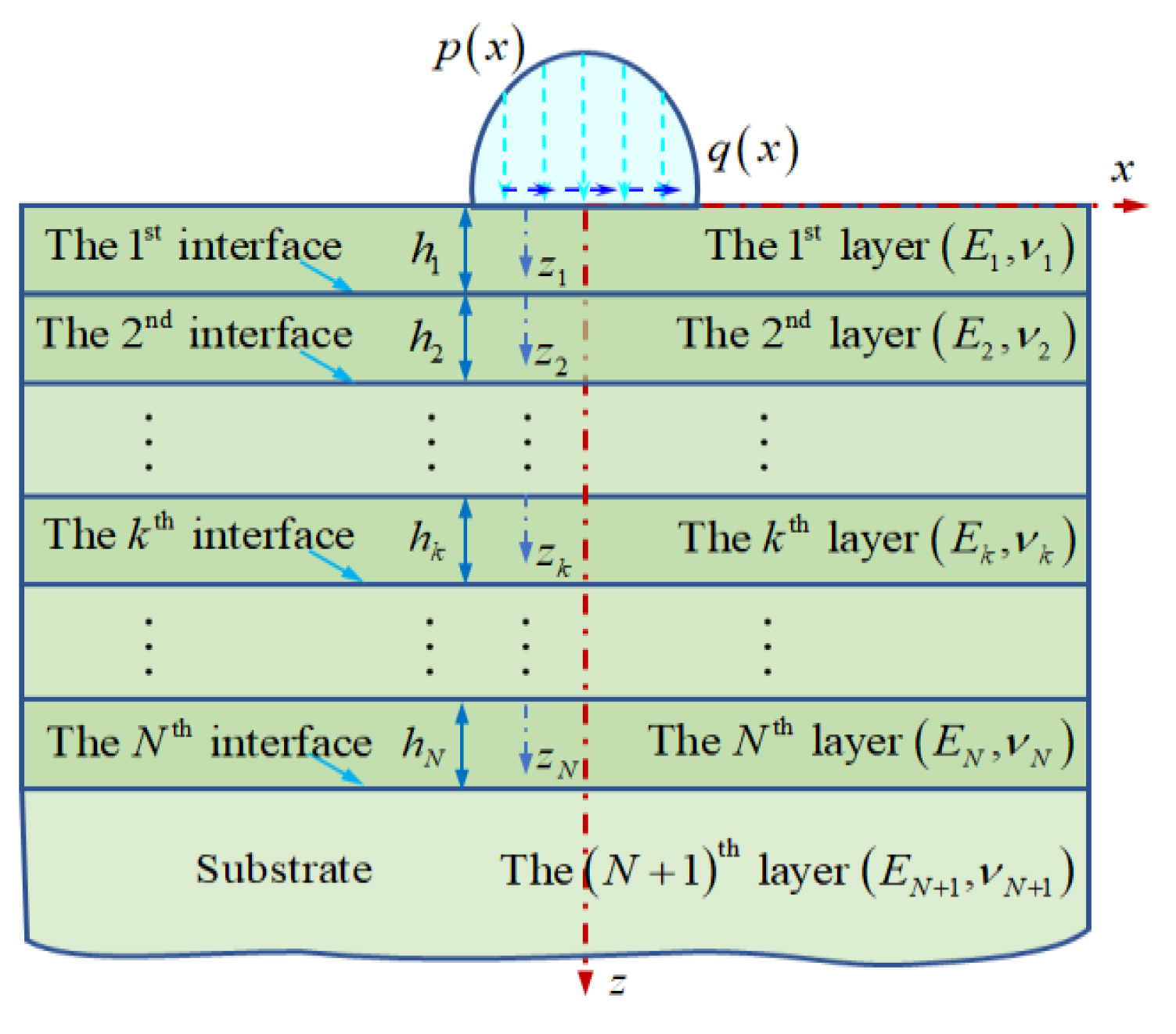
2.1. Statement of the Mechanical Problem

Figure 1 illustrates a 2D plain strain problem, in which an elastic solid coated with multilayers is subjected to surface contact loading p(x) and q(x). In the figure, N is the layer number of the multilayer coatings, while h_k, E_k and ν_k are the thickness, elasticity modulus and Poisson ratio of the kth layer, respectively. E_N+1 and ν_N+1 are the elasticity modulus and Poisson ratio of the substrate material, respectively. p(x) and q(x) are the surface normal pressure and the tangential traction applied on the surface of the multilayer coatings, respectively. The normal pressure and the tangential traction applied on the surface are given by Hertz line contact theory as follows [29]:

$$p\left(x\right)=\{\begin{array}{cc}{p}_{\mathrm{H}}\sqrt{{b_{\mathrm{H}}}^2-x^2}& \left|x\right|\le b_{\mathrm{H}}\\ 0& \mathrm{else}\end{array}$$

(1)

$$q\left(x\right)=\{\begin{array}{cc}{\mathsf{\mu }}_f{p}_{\mathrm{H}}\sqrt{{b_{\mathrm{H}}}^2-x^2}& \left|x\right|\le b_{\mathrm{H}}\\ 0& \mathrm{else}\end{array}$$

(2)

where p_H and b_H represent the maximum contact pressure and the contact half-width of the substrate material in the Hertz line contact, and μ_f represents the friction coefficient.

2.2. Two-Dimensional Analytical Frequency Response Functions of Multilayered Solids

For a 2D plane strain problem, the stress and displacement components of layered materials in frequency domain are given as Equations (3)–(7) [22,23] based on the Airy stress function by using the FT technique.

$${\tilde{\mathsf{\sigma }}}_{zz}^{\left(k\right)}=-{{\mathsf{\omega }}_x}^2{A}_1^{\left(k\right)}{\mathrm{e}}^{-\left|{\mathsf{\omega }}_x\right|z_k}-{{\mathsf{\omega }}_x}^2{A}_2^{\left(k\right)}{z}_k{\mathrm{e}}^{-\left|{\mathsf{\omega }}_x\right|z_k}-{{\mathsf{\omega }}_x}^2{A}_3^{\left(k\right)}{\mathrm{e}}^{\left|{\mathsf{\omega }}_x\right|z_k}-{{\mathsf{\omega }}_x}^2{A}_4^{\left(k\right)}{z}_k{\mathrm{e}}^{\left|{\mathsf{\omega }}_x\right|z_k}$$

(3)

$${\tilde{\mathsf{\sigma }}}_{xx}^{\left(k\right)}={\left|{\mathsf{\omega }}_x\right|}^2{A}_1^{\left(k\right)}{\mathrm{e}}^{-\left|{\mathsf{\omega }}_x\right|z_k}-\left(2-\left|{\mathsf{\omega }}_x\right|z_k\right)\left|{\mathsf{\omega }}_x\right|A_2^{\left(k\right)}{\mathrm{e}}^{-\left|{\mathsf{\omega }}_x\right|z_k}+{\left|{\mathsf{\omega }}_x\right|}^2{A}_3^{\left(k\right)}{\mathrm{e}}^{\left|{\mathsf{\omega }}_x\right|z_k}+\left(2+\left|{\mathsf{\omega }}_x\right|z_k\right)\left|{\mathsf{\omega }}_x\right|A_4^{\left(k\right)}{\mathrm{e}}^{\left|{\mathsf{\omega }}_x\right|z_k}$$

(4)

$${\tilde{\mathsf{\sigma }}}_{xz}^{\left(k\right)}=\mathrm{i}{\mathsf{\omega }}_x\left(\left|{\mathsf{\omega }}_x\right|A_1^{\left(k\right)}{\mathrm{e}}^{-\left|{\mathsf{\omega }}_x\right|z_k}-\left(1-\left|{\mathsf{\omega }}_x\right|z_k\right)A_2^{\left(k\right)}{\mathrm{e}}^{-\left|{\mathsf{\omega }}_x\right|z_k}-\left|{\mathsf{\omega }}_x\right|A_3^{\left(k\right)}{\mathrm{e}}^{\left|{\mathsf{\omega }}_x\right|z_k}-\left(1+\left|{\mathsf{\omega }}_x\right|z_k\right)A_4^{\left(k\right)}{\mathrm{e}}^{\left|{\mathsf{\omega }}_x\right|z_k}\right)$$

(5)

$${\tilde{u}}_z^{\left(k\right)}=\frac{1+{\mathsf{\nu }}_k}{E_k}\left(\begin{array}{l}\left|{\mathsf{\omega }}_x\right|A_1^{\left(k\right)}{\mathrm{e}}^{-\left|{\mathsf{\omega }}_x\right|z_k}+\left(1-2{\mathsf{\nu }}_k+\left|{\mathsf{\omega }}_x\right|z_k\right)A_2^{\left(k\right)}{\mathrm{e}}^{-\left|{\mathsf{\omega }}_x\right|z_k}\\ -\left|{\mathsf{\omega }}_x\right|A_3^{\left(k\right)}{\mathrm{e}}^{\left|{\mathsf{\omega }}_x\right|z_k}+\left(1-2{\mathsf{\nu }}_k-\left|{\mathsf{\omega }}_x\right|z_k\right)A_4^{\left(k\right)}{\mathrm{e}}^{\left|{\mathsf{\omega }}_x\right|z_k}\end{array}\right)$$

(6)

$${\tilde{u}}_x^{\left(k\right)}=-\mathrm{i}\frac{1+{\mathsf{\nu }}_k}{E_k}\left[\begin{array}{l}{\mathsf{\omega }}_x{A}_1^{\left(k\right)}{\mathrm{e}}^{-\left|{\mathsf{\omega }}_x\right|z_k}+\left({\mathsf{\omega }}_x{z}_k-2\left(1-{\mathsf{\nu }}_k\right)\left|{\mathsf{\omega }}_x\right|/{\mathsf{\omega }}_x\right)A_2^{\left(k\right)}{\mathrm{e}}^{-\left|{\mathsf{\omega }}_x\right|z_k}\\ +{\mathsf{\omega }}_x{A}_3^{\left(k\right)}{\mathrm{e}}^{\left|{\mathsf{\omega }}_x\right|z_k}+\left({\mathsf{\omega }}_x{z}_k+2\left(1-{\mathsf{\nu }}_k\right)\left|{\mathsf{\omega }}_x\right|/{\mathsf{\omega }}_x\right)A_4^{\left(k\right)}{\mathrm{e}}^{\left|{\mathsf{\omega }}_x\right|z_k}\end{array}\right]$$

(7)

where the symbol ‘i’ represents the imaginary unit, the symbol ‘~’ represents the one-dimensional Fourier integral transform. A₁^(k), A₂^(k), A₃^(k) are A₄^(k) are the unknown constants in the 2D FRF of the kth layered material.

There are 4(N + 1) − 2 unknown constants that need to be determined in total to obtain the 2D FRF of a multilayered solid with N layers, since the unknown constants A₃^(k) and A₄^(k) are zero because all the stress and displacement components of the substrate become zero when z_N+1 tends to infinity. The 4(N + 1) − 2 unknown constants can be determined with the boundary conditions and the interface continuous conditions of the multilayered solids, which are:

$${{\tilde{\mathsf{\sigma }}}_{zz}^{\left(1\right)}|}_{z_1=0}=-\tilde{p}$$

(8)

$${{\tilde{\mathsf{\sigma }}}_{zx}^{\left(1\right)}|}_{z_1=0}=-\tilde{q}$$

(9)

$${{\tilde{\mathsf{\sigma }}}_{zz}^{\left(k\right)}|}_{z_k=h_k}={{\tilde{\mathsf{\sigma }}}_{zz}^{\left(k+1\right)}|}_{z_{k+1}=0}$$

(10)

$${{\tilde{\mathsf{\sigma }}}_{zx}^{\left(k\right)}|}_{z_k=h_k}={{\tilde{\mathsf{\sigma }}}_{zx}^{\left(k+1\right)}|}_{z_{k+1}=0}$$

(11)

$${{\tilde{u}}_z^{\left(k\right)}|}_{z_k=h_k}={{\tilde{u}}_z^{\left(k+1\right)}|}_{z_{k+1}=0}$$

(12)

$${{\tilde{u}}_x^{\left(k\right)}|}_{z_k=h_k}={{\tilde{u}}_x^{\left(k+1\right)}|}_{z_{k+1}=0}$$

(13)

where 1 ≤ k ≤ N, $\tilde{p}$ and $\tilde{q}$ are the one-dimensional FT of the normal pressure p(x) and the tangential traction q(x). Using the results given in Ref. [30,31], the one-dimensional FT of the normal pressure p(x) and the tangential traction q(x) can be given as Equations (14) and (15), respectively.

$$\tilde{p}=\mathsf{\pi }{p}_{\mathrm{H}}{J}_1\left(b_{\mathrm{H}}{\mathsf{\omega }}_x\right)/{\mathsf{\omega }}_x$$

(14)

$$\tilde{q}=\mathsf{\pi }{\mathsf{\mu }}_f{p}_{\mathrm{H}}{J}_1\left(b_{\mathrm{H}}{\mathsf{\omega }}_x\right)/{\mathsf{\omega }}_x$$

(15)

where J₁ is the Bessel function of the first kind.

Substituting Equations (3)–(7) into Equations (8) and (9), two linear equations are obtained:

$$A_1^{\left(1\right)}+A_3^{\left(1\right)}=-\tilde{p}/{{\mathsf{\omega }}_x}^2$$

(16)

$$\left|{\mathsf{\omega }}_x\right|A_1^{\left(1\right)}-A_2^{\left(1\right)}-\left|{\mathsf{\omega }}_x\right|A_3^{\left(1\right)}-A_4^{\left(1\right)}=\mathrm{i}\tilde{q}/{\mathsf{\omega }}_x$$

(17)

When 1 ≤ k ≤ N − 1, 4(N − 1) linear equations can be obtained by substituting Equations (3)–(7) into Equations (10)–(13).

$${\mathrm{e}}^{-\left|{\mathsf{\omega }}_x\right|h_k}{A}_1^{\left(k\right)}+h_k{\mathrm{e}}^{-\left|{\mathsf{\omega }}_x\right|h_k}{A}_2^{\left(k\right)}+{\mathrm{e}}^{\left|{\mathsf{\omega }}_x\right|h_k}{A}_3^{\left(k\right)}+A_4^{\left(k\right)}{h}_k{\mathrm{e}}^{\left|{\mathsf{\omega }}_x\right|h_k}-A_1^{\left(k+1\right)}-A_3^{\left(k+1\right)}=0$$

(18)

$$\begin{array}{r}-\left|{\mathsf{\omega }}_x\right|{\mathrm{e}}^{-\left|{\mathsf{\omega }}_x\right|h_k}{A}_1^{\left(k\right)}+\left(1-\left|{\mathsf{\omega }}_x\right|h_k\right){\mathrm{e}}^{-\left|{\mathsf{\omega }}_x\right|h_k}{A}_2^{\left(k\right)}+\left|{\mathsf{\omega }}_x\right|{\mathrm{e}}^{\left|{\mathsf{\omega }}_x\right|h_k}{A}_3^{\left(k\right)}+\left(1+\left|{\mathsf{\omega }}_x\right|h_k\right){\mathrm{e}}^{\left|{\mathsf{\omega }}_x\right|h_k}{A}_4^{\left(k\right)}\\ +\left|{\mathsf{\omega }}_x\right|A_1^{\left(k+1\right)}-A_2^{\left(k+1\right)}-\left|{\mathsf{\omega }}_x\right|A_3^{\left(k+1\right)}-A_4^{\left(k+1\right)}=0\end{array}$$

(19)

$$\begin{array}{r}\left|{\mathsf{\omega }}_x\right|A_1^{\left(k\right)}{\mathrm{e}}^{-\left|{\mathsf{\omega }}_x\right|h_k}+\left(1-2{\mathsf{\nu }}_k+\left|{\mathsf{\omega }}_x\right|h_k\right)A_2^{\left(k\right)}{\mathrm{e}}^{-\left|{\mathsf{\omega }}_x\right|h_k}-\left|{\mathsf{\omega }}_x\right|A_3^{\left(k\right)}{\mathrm{e}}^{\left|{\mathsf{\omega }}_x\right|h_k}+\left(1-2{\mathsf{\nu }}_k-\left|{\mathsf{\omega }}_x\right|h_k\right)A_4^{\left(k\right)}{\mathrm{e}}^{\left|{\mathsf{\omega }}_x\right|h_k}\\ -{\mathsf{\xi }}_{k+1}\left|{\mathsf{\omega }}_x\right|A_1^{\left(k+1\right)}-{\mathsf{\xi }}_{k+1}\left(1-2{\mathsf{\nu }}_{k+1}\right)A_2^{\left(k+1\right)}-{\mathsf{\xi }}_{k+1}\left|{\mathsf{\omega }}_x\right|A_3^{\left(k+1\right)}-{\mathsf{\xi }}_{k+1}\left(1-2{\mathsf{\nu }}_{k+1}\right)A_4^{\left(k+1\right)}=0\end{array}$$

(20)

$$\begin{array}{r}{\mathsf{\omega }}_x{A}_1^{\left(k\right)}{\mathrm{e}}^{-\left|{\mathsf{\omega }}_x\right|h_k}+\left({\mathsf{\omega }}_x{h}_k-2\left(1-{\mathsf{\nu }}_k\right)\left|{\mathsf{\omega }}_x\right|/{\mathsf{\omega }}_x\right)A_2^{\left(k\right)}{\mathrm{e}}^{-\left|{\mathsf{\omega }}_x\right|h_k}\\ +{\mathsf{\omega }}_x{A}_3^{\left(k\right)}{\mathrm{e}}^{\left|{\mathsf{\omega }}_x\right|h_k}+\left({\mathsf{\omega }}_x{h}_k+2\left(1-{\mathsf{\nu }}_k\right)\left|{\mathsf{\omega }}_x\right|/{\mathsf{\omega }}_x\right)A_4^{\left(k\right)}{\mathrm{e}}^{\left|{\mathsf{\omega }}_x\right|h_k}-{\mathsf{\xi }}_{k+1}{\mathsf{\omega }}_x{A}_1^{\left(k+1\right)}\\ +\left(2{\mathsf{\xi }}_{k+1}\left(1-{\mathsf{\nu }}_{k+1}\right)\left|{\mathsf{\omega }}_x\right|/{\mathsf{\omega }}_x\right)A_2^{\left(k+1\right)}-{\mathsf{\xi }}_{k+1}{\mathsf{\omega }}_x{A}_3^{\left(k+1\right)}-\left(2{\mathsf{\xi }}_{k+1}\left(1-{\mathsf{\nu }}_{k+1}\right)\left|{\mathsf{\omega }}_x\right|/{\mathsf{\omega }}_x\right)A_4^{\left(k+1\right)}=0\end{array}$$

(21)

When k = N, 4 linear equations can be obtained by substituting Equations (3)–(7) into Equations (10)–(13).

$${\mathrm{e}}^{-\left|{\mathsf{\omega }}_x\right|h_N}{A}_1^{\left(N\right)}+h_N{\mathrm{e}}^{-\left|{\mathsf{\omega }}_x\right|h_N}{A}_2^{\left(N\right)}+{\mathrm{e}}^{\left|{\mathsf{\omega }}_x\right|h_N}{A}_3^{\left(N\right)}+A_4^{\left(N\right)}{h}_N{\mathrm{e}}^{\left|{\mathsf{\omega }}_x\right|h_N}-A_1^{\left(N+1\right)}=0$$

(22)

$$\begin{array}{r}-\left|{\mathsf{\omega }}_x\right|{\mathrm{e}}^{-\left|{\mathsf{\omega }}_x\right|h_N}{A}_1^{\left(N\right)}+\left(1-\left|{\mathsf{\omega }}_x\right|h_N\right){\mathrm{e}}^{-\left|{\mathsf{\omega }}_x\right|h_N}{A}_2^{\left(N\right)}+\left|{\mathsf{\omega }}_x\right|{\mathrm{e}}^{\left|{\mathsf{\omega }}_x\right|h_N}{A}_3^{\left(N\right)}+\left(1+\left|{\mathsf{\omega }}_x\right|h_N\right){\mathrm{e}}^{\left|{\mathsf{\omega }}_x\right|h_N}{A}_4^{\left(N\right)}\\ +\left|{\mathsf{\omega }}_x\right|A_1^{\left(N+1\right)}-A_2^{\left(N+1\right)}=0\hspace{0.17em}\end{array}$$

(23)

$$\begin{array}{r}\left|{\mathsf{\omega }}_x\right|A_1^{\left(N\right)}{\mathrm{e}}^{-\left|{\mathsf{\omega }}_x\right|h_N}+\left(1-2{\mathsf{\nu }}_N+\left|{\mathsf{\omega }}_x\right|h_N\right)A_2^{\left(N\right)}{\mathrm{e}}^{-\left|{\mathsf{\omega }}_x\right|h_N}-\left|{\mathsf{\omega }}_x\right|A_3^{\left(N\right)}{\mathrm{e}}^{\left|{\mathsf{\omega }}_x\right|h_N}\\ +\left(1-2{\mathsf{\nu }}_N-\left|{\mathsf{\omega }}_x\right|h_N\right)A_4^{\left(N\right)}{\mathrm{e}}^{\left|{\mathsf{\omega }}_x\right|h_N}-{\mathsf{\xi }}_{N+1}\left|{\mathsf{\omega }}_x\right|A_1^{\left(N+1\right)}-{\mathsf{\xi }}_{N+1}\left(1-2{\mathsf{\nu }}_{N+1}\right)A_2^{\left(N+1\right)}=0\end{array}$$

(24)

$$\begin{array}{r}{\mathsf{\omega }}_x{A}_1^{\left(N\right)}{\mathrm{e}}^{-\left|{\mathsf{\omega }}_x\right|h_N}+\left({\mathsf{\omega }}_x{h}_N-2\left(1-{\mathsf{\nu }}_N\right)\left|{\mathsf{\omega }}_x\right|/{\mathsf{\omega }}_x\right)A_2^{\left(N\right)}{\mathrm{e}}^{-\left|{\mathsf{\omega }}_x\right|h_N}+{\mathsf{\omega }}_x{A}_3^{\left(N\right)}{\mathrm{e}}^{\left|{\mathsf{\omega }}_x\right|h_N}\\ +\left({\mathsf{\omega }}_x{h}_N+2\left(1-{\mathsf{\nu }}_N\right)\left|{\mathsf{\omega }}_x\right|/{\mathsf{\omega }}_x\right)A_4^{\left(N\right)}{\mathrm{e}}^{\left|{\mathsf{\omega }}_x\right|h_N}-{\mathsf{\xi }}_{N+1}{\mathsf{\omega }}_x{A}_1^{\left(N+1\right)}+\left(2{\mathsf{\xi }}_{N+1}\left(1-{\mathsf{\nu }}_{N+1}\right)\left|{\mathsf{\omega }}_x\right|/{\mathsf{\omega }}_x\right)A_2^{\left(N+1\right)}=0\end{array}$$

(25)

where ξ_k+1 = E_k(1 + ν_k+1)/[E_k+1(1 + ν_k+1)].

The system of linear equations composed of Equations (16)–(25) can be solved simultaneously with a numerical method according to Ref. [32]. However, the numerical method will consume a lot solving time especially when the layer number is large, since an equation group with 4(N + 1) − 2 equations should be solved for λN_x times. The meaning of the symols λ and N_x can be seen in Section 2.3. Therefore, analogous to the method proposed in Ref. [33], an analytical solution of the unknown constants in Equations (3)–(7) is derived and given in a recursive form in this paper. Equations (22)–(25) based on the continuous conditions of the last interface are used to solved the unknown constants A₁^(N+1) and A₂^(N+1) of the substrate as functions of the unknown constants A₁^(k), A₂^(k), A₃^(k), and A₄^(k) of the kth layer.

$$A_1^{\left(N+1\right)}{=\mathrm{e}}^{-\left|{\mathsf{\omega }}_x\right|h_N}{A}_1^{\left(N\right)}+h_N{\mathrm{e}}^{-\left|{\mathsf{\omega }}_x\right|h_N}{A}_2^{\left(N\right)}+{\mathrm{e}}^{\left|{\mathsf{\omega }}_x\right|h_N}{A}_3^{\left(N\right)}+h_N{\mathrm{e}}^{\left|{\mathsf{\omega }}_x\right|h_N}{A}_4^{\left(N\right)}$$

(26)

$$A_2^{\left(N+1\right)}={\mathrm{e}}^{-\left|{\mathsf{\omega }}_x\right|h_N}{A}_2^{\left(N\right)}+2\left|{\mathsf{\omega }}_x\right|{\mathrm{e}}^{\left|{\mathsf{\omega }}_x\right|h_N}{A}_3^{\left(N\right)}+\left(1+2\left|{\mathsf{\omega }}_x\right|h_N\right){\mathrm{e}}^{\left|{\mathsf{\omega }}_x\right|h_N}{A}_4^{\left(N\right)}$$

(27)

Two more relationships of the unknown constants A₁^(N), A₂^(N), A₃^(N) and A₄^(N) are given as:

$$S_1^{\left(N\right)}{A}_1^{\left(N\right)}+S_2^{\left(N\right)}{S}_2^{\left(N\right)}+S_3^{\left(N\right)}{\mathrm{e}}^{2\left|{\mathsf{\omega }}_x\right|h_N}{A}_3^{\left(N\right)}+S_4^{\left(N\right)}{\mathrm{e}}^{2\left|{\mathsf{\omega }}_x\right|h_N}{A}_4^{\left(N\right)}=0$$

(28)

$$S_5^{\left(N\right)}{A}_1^{\left(N\right)}+S_6^{\left(N\right)}{S}_2^{\left(N\right)}+S_7^{\left(N\right)}{\mathrm{e}}^{2\left|{\mathsf{\omega }}_x\right|h_N}{A}_3^{\left(N\right)}+S_8^{\left(N\right)}{\mathrm{e}}^{2\left|{\mathsf{\omega }}_x\right|h_N}{A}_4^{\left(N\right)}=0$$

(29)

where the S terms in Equations (28) and (29) are the intermediate constants which are listed in the Appendix A.

The unknown constants A₁^(k+1), A₂^(k+1), A₃^(k+1), and A₄^(k+1) of the (k + 1)th layer can be solved from Equations (18)–(21) as functions of the unknown constants A₁^(k), A₂^(k), A₃^(k), and A₄^(k) of the kth layer as follows:

$$A_1^{\left(k+1\right)}=t_{11}^{\left(k\right)}{\mathrm{e}}^{-\left|{\mathsf{\omega }}_x\right|h_k}{A}_1^{\left(k\right)}+t_{12}^{\left(k\right)}{\mathrm{e}}^{-\left|{\mathsf{\omega }}_x\right|h_k}{A}_2^{\left(k\right)}+t_{13}^{\left(k\right)}{\mathrm{e}}^{\left|{\mathsf{\omega }}_x\right|h_k}{A}_3^{\left(k\right)}+t_{14}^{\left(k\right)}{\mathrm{e}}^{\left|{\mathsf{\omega }}_x\right|h_k}{A}_4^{\left(k\right)}$$

(30)

$$A_2^{\left(k+1\right)}=t_{21}^{\left(k\right)}{\mathrm{e}}^{-\left|{\mathsf{\omega }}_x\right|h_k}{A}_1^{\left(k\right)}+t_{22}^{\left(k\right)}{\mathrm{e}}^{-\left|{\mathsf{\omega }}_x\right|h_k}{A}_2^{\left(k\right)}+t_{23}^{\left(k\right)}{\mathrm{e}}^{\left|{\mathsf{\omega }}_x\right|h_k}{A}_3^{\left(k\right)}+t_{24}^{\left(k\right)}{\mathrm{e}}^{\left|{\mathsf{\omega }}_x\right|h_k}{A}_4^{\left(k\right)}$$

(31)

$$A_3^{\left(k+1\right)}=t_{31}^{\left(k\right)}{\mathrm{e}}^{-\left|{\mathsf{\omega }}_x\right|h_k}{A}_1^{\left(k\right)}+t_{32}^{\left(k\right)}{\mathrm{e}}^{-\left|{\mathsf{\omega }}_x\right|h_k}{A}_2^{\left(k\right)}+t_{33}^{\left(k\right)}{\mathrm{e}}^{\left|{\mathsf{\omega }}_x\right|h_k}{A}_3^{\left(k\right)}+t_{34}^{\left(k\right)}{\mathrm{e}}^{\left|{\mathsf{\omega }}_x\right|h_k}{A}_4^{\left(k\right)}$$

(32)

$$A_4^{\left(k+1\right)}=t_{41}^{\left(k\right)}{\mathrm{e}}^{-\left|{\mathsf{\omega }}_x\right|h_k}{A}_1^{\left(k\right)}+t_{42}^{\left(k\right)}{\mathrm{e}}^{-\left|{\mathsf{\omega }}_x\right|h_k}{A}_2^{\left(k\right)}+t_{43}^{\left(k\right)}{\mathrm{e}}^{\left|{\mathsf{\omega }}_x\right|h_k}{A}_3^{\left(k\right)}+t_{44}^{\left(k\right)}{\mathrm{e}}^{\left|{\mathsf{\omega }}_x\right|h_k}{A}_4^{\left(k\right)}$$

(33)

where the t terms in Equations (30)–(33) are the intermediate constants which are also listed in the Appendix A.

Assume that two relationships of the unknown constants A₁^(k+1), A₂^(k+1), A₃^(k+1), and A₄^(k+1) of the (k + 1)th layer have been developed as follows:

$$S_1^{\left(k+1\right)}{A}_1^{\left(k+1\right)}+S_2^{\left(k+1\right)}{A}_2^{\left(k+1\right)}+S_3^{\left(k+1\right)}{\mathrm{e}}^{2\left|{\mathsf{\omega }}_x\right|h_{k+1}}{A}_3^{\left(k+1\right)}+S_4^{\left(k+1\right)}{\mathrm{e}}^{2\left|{\mathsf{\omega }}_x\right|h_{k+1}}{A}_4^{\left(k+1\right)}=0$$

(34)

$$S_5^{\left(k+1\right)}{A}_1^{\left(k+1\right)}+S_6^{\left(k+1\right)}{A}_2^{\left(k+1\right)}+S_7^{\left(k+1\right)}{\mathrm{e}}^{2\left|{\mathsf{\omega }}_x\right|h_{k+1}}{A}_3^{\left(k+1\right)}+S_8^{\left(k+1\right)}{\mathrm{e}}^{2\left|{\mathsf{\omega }}_x\right|h_{k+1}}{A}_4^{\left(k+1\right)}=0$$

(35)

By appropriate algebra operations among the equations shown in Equations (30)–(35), two relationships of the unknown constants A₁^(k), A₂^(k), A₃^(k), and A₄^(k) of the kth layer can be deduced as follows:

$$S_1^{\left(k\right)}{A}_1^{\left(k\right)}+S_2^{\left(k\right)}{A}_2^{\left(k\right)}+S_3^{\left(k\right)}{\mathrm{e}}^{2\left|{\mathsf{\omega }}_x\right|h_k}{A}_3^{\left(k\right)}+S_4^{\left(k\right)}{\mathrm{e}}^{2\left|{\mathsf{\omega }}_x\right|h_k}{A}_4^{\left(k\right)}=0$$

(36)

$$S_5^{\left(k\right)}{A}_1^{\left(k\right)}+S_6^{\left(k\right)}{A}_2^{\left(k\right)}+S_7^{\left(k\right)}{\mathrm{e}}^{2\left|{\mathsf{\omega }}_x\right|h_k}{A}_3^{\left(k\right)}+S_8^{\left(k\right)}{\mathrm{e}}^{2\left|{\mathsf{\omega }}_x\right|h_k}{A}_4^{\left(k\right)}=0$$

(37)

where the S terms in Equations (36) and (37) are the intermediate constants and listed in the Appendix A. It can be found that the S terms of the kth layer contain those of the (k + 1)th layer and their algebraic expressions are true for every layer of the multilayer system. Therefore, the two relationships of the unknown constants A₁¹, A₂¹, A₃¹, and A₄¹ of the 1st layer are:

$$S_1^{\left(1\right)}{A}_1^{\left(1\right)}+S_2^{\left(k\right)}{A}_2^{\left(k\right)}+S_3^{\left(1\right)}{\mathrm{e}}^{2\left|{\mathsf{\omega }}_x\right|h_1}{A}_3^{\left(1\right)}+S_4^{\left(1\right)}{\mathrm{e}}^{2\left|{\mathsf{\omega }}_x\right|h_1}{A}_4^{\left(1\right)}=0$$

(38)

$$S_5^{\left(1\right)}{A}_1^{\left(1\right)}+S_6^{\left(1\right)}{A}_2^{\left(1\right)}+S_7^{\left(1\right)}{\mathrm{e}}^{2\left|{\mathsf{\omega }}_x\right|h_1}{A}_3^{\left(1\right)}+S_8^{\left(1\right)}{\mathrm{e}}^{2\left|{\mathsf{\omega }}_x\right|h_1}{A}_4^{\left(1\right)}=0$$

(39)

The S terms of the 1st layer in Equations (36) and (37) are calculated with their recursive formulas shown in Equations (A1)–(A8) and Equations (A24)–(A32) layer by layer in a down to top fashion. The solution of the unknown constants A₁¹, A₂¹, A₃¹, and A₄¹ of the 1st layer can be solved from Equations (16), (17), (38), and (39), and given as follows:

$$A_1^{\left(1\right)}=\left(S_4^{\left(0\right)}{R}_a^{\left(0\right)}-S_2^{\left(0\right)}{R}_b^{\left(0\right)}\right)/\left(S_1^{\left(0\right)}{S}_4^{\left(0\right)}-S_2^{\left(0\right)}{S}_3^{\left(0\right)}\right)$$

(40)

$$A_2^{\left(1\right)}=\left(S_3^{\left(0\right)}{R}_a^{\left(0\right)}-S_1^{\left(0\right)}{R}_b^{\left(0\right)}\right)/\left(S_2^{\left(0\right)}{S}_3^{\left(0\right)}-S_1^{\left(0\right)}{S}_4^{\left(0\right)}\right)$$

(41)

$$A_3^{\left(1\right)}=-\tilde{p}/{{\mathsf{\omega }}_x}^2-A_1^{\left(1\right)}$$

(42)

$$A_4^{\left(1\right)}=\left|{\mathsf{\omega }}_x\right|A_1^{\left(1\right)}-A_2^{\left(1\right)}-\left|{\mathsf{\omega }}_x\right|A_3^{\left(1\right)}-\mathrm{i}\tilde{q}/{\mathsf{\omega }}_x$$

(43)

where S₁⁽⁰⁾, S₂⁽⁰⁾, S₃⁽⁰⁾, S₄⁽⁰⁾, R_a⁽⁰⁾, and R_b⁽⁰⁾ are the intermediate constants and listed in the Appendix A.

Then the unknown constants in the 2D general FRF of the other layers and the substrate can be obtained with their recursive formulas shown in Equations (28) and (29) and Equations (22)–(25) layer by layer in a top-down fashion.

2.3. Numerical Conversion Method

Having obtained the 2D explicit analytical FRF of multilayered solids, the elastic field solution in the space domain can be converted from its corresponding FRF by using an IFFT based numerical conversion method. The conversion method originally is used to produce the influence coefficients of the stress and displacement components for developing a semi-analytical contact model [34,35]. The detailed steps of using the IFFT based numerical conversion method to produce the stress component σ_rs at z depth are as follows:

• Select a computing domain {x|x_b ≤ x ≤ x_e} at z depth and divide it uniformly into N_x line elements. The number N_x is required to be a positive integral power of 2. x_b and x_e are usually chosen to be −2b_H and 2b_H, respectively.
• Refine the grid into N_ωx uniform elements in the frequency domain {ω_x|−π < ω_x ≤ π}, where N_ωx = λN_x and λ should be a nonnegative integral power of 2.
• Construct a discrete series ${\widehat{\mathsf{\sigma }}}_{rs}$ by using the FRF of the stress component σ_rs:

  $${\widehat{\mathsf{\sigma }}}_{rs}\left[i\right]=\frac{{\mathsf{\Delta }}_{{\mathsf{\omega }}_x}{N}_{{\mathsf{\omega }}_x}}{2\mathsf{\pi }}{\displaystyle \sum _{\mathsf{\zeta }=-\mathsf{\kappa }}^{\mathsf{\kappa }}{\tilde{\mathsf{\sigma }}}_{rs}\left(i{\mathsf{\Delta }}_{{\mathsf{\omega }}_x}-{\mathsf{\Delta }}_{{\mathsf{\omega }}_x}{N}_{{\mathsf{\omega }}_x}\mathsf{\zeta }\right)}\hspace{0.17em}-N_{{\mathsf{\omega }}_x}/2<i\le N_{{\mathsf{\omega }}_x}/2$$

  (44)
• Reconstruct a new discrete series ${\stackrel{⌢}{\mathsf{\sigma }}}_{rs}$ by applying a wrap-order operation to ${\stackrel{⌢}{\mathsf{\sigma }}}_{rs}$:

  $$\begin{array}{l}{\stackrel{⌢}{\mathsf{\sigma }}}_{rs}\left[i\right]={\widehat{\mathsf{\sigma }}}_{rs}\left[i+N_{{\mathsf{\omega }}_x}/2-1\right]\hspace{0.17em}\hspace{0.17em}\hspace{0.17em}\hspace{0.17em}\hspace{0.17em}\hspace{0.17em}\hspace{0.17em}{N}_{{\mathsf{\omega }}_x}/2<i\le 1\\ {\stackrel{⌢}{\mathsf{\sigma }}}_{rs}\left[i\right]={\widehat{\mathsf{\sigma }}}_{rs}\left[i-N_{{\mathsf{\omega }}_x}/2-1\right]\hspace{0.17em}\hspace{0.17em}\hspace{0.17em}\hspace{0.17em}\hspace{0.17em}\hspace{0.17em}\hspace{0.17em}2<i\le N_{{\mathsf{\omega }}_x}/2\end{array}$$

  (45)
• Apply the IFFT operation to the discrete series ${\stackrel{⌢}{\mathsf{\sigma }}}_{rs}$:

  $${\overline{\mathsf{\sigma }}}_{rs}=\mathrm{IFFT}\left({\stackrel{⌢}{\mathsf{\sigma }}}_{rs}\right)$$

  (46)
• The stress at each line element in the discrete space domain can be obtained as follows:

  $$\begin{array}{l}{\mathsf{\sigma }}_{rs}\left[i\right]={\overline{\mathsf{\sigma }}}_{rs}\left[N_{{\mathsf{\omega }}_x}-N_x/2+i+1\right]\hspace{0.17em}\hspace{0.17em}\hspace{0.17em}\hspace{0.17em}\hspace{0.17em}1\le i\le N_x/2-1\\ {\mathsf{\sigma }}_{rs}\left[i\right]={\overline{\mathsf{\sigma }}}_{rs}\left[i-N_x/2+1\right]\hspace{0.17em}\hspace{0.17em}\hspace{0.17em}\hspace{0.17em}\hspace{0.17em}\hspace{0.17em}\hspace{0.17em}\hspace{0.17em}\hspace{0.17em}\hspace{0.17em}\hspace{0.17em}\hspace{0.17em}\hspace{0.17em}{N}_x/2\le i\le N_x-1\end{array}$$

  (47)

A very high conversion accuracy can be achieved by selecting an enough large λ and κ to eliminate the periodic error and the error caused by aliasing effect. However, the increase of λ and κ will lead to a heavier calculation burden. In this paper, λ and κ are fixed as 4 and 5, respectively because the elastic field solution of the present method agrees well with the exact analytical solution given by McEwen [36] and the solution of the finite element method, when λ = 4 and κ = 5. It can be found in Section 3 of this paper.

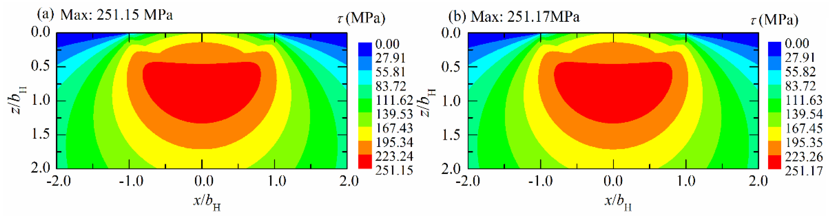
3. Validation of the Present Method

In order to validate the present method, the maximum shear stress in the subsurface of a half plane of the substrate material subjected to surface mechanical loading obtained by the present method is compared with the exact analytical solution given by McEwen seen in Ref. [36]. The input parameters of the present method are listed in

Table 1. Input parameters of the present method for simulating a half plane of the substrate material subjected to subjected to surface contact loading.

pH (Mpa)	bH (mm)	N (–)	νi (1 ≤ i ≤ N + 1) (–)	Ei (1 ≤ i ≤ N + 1) (GPa)	hi (1 ≤ i ≤ N) (m)	μf (–)
836.41	0.761	3	0.3	200	bH/N	0

. The elasticity parameters of the layer are the same to those of the substrate when the present method is adopted to simulate the problem of the half plane of the substrate material subjected to surface contact loading.

Figure 2 is the contour plots of the maximum shear stress of the half plane of the substrate material subjected to surface contact loading. When the friction coefficient is 0. As indicated in the figure, the contour plot of the maximum shear stress τ of the present method shown in Figure 2b agrees well with the exact analytical solution given by McEwen shown in Figure 2a. The relative error of the peak value of the maximum shear stress is not more than 0.01%.

In order to further validate the present method, a comparison of the maximum shear stress in the subsurface of a multilayered solid with 40 layers is also conducted between the solution of the present method and that of the finite element method. The parameters of the multilayered solid and the other concerning parameters are shown in

Table 2. Input parameters of the present method for simulating the multilayered solid with 40 layers subjected to surface contact loading.

pH (Mpa)	bH (mm)	N (–)	νi (1 ≤ i ≤ N + 1) (–)	E41 (GPa)	E1 (GPa)	Ei (2 ≤ i ≤ N) (GPa)	hi (1 ≤ i ≤ N) (m)	μf (–)
836.41	0.761	40	0.3	200	100	Ei = Ei−1 + ΔE	bH/N	0, 0.2

.

The finite element analysis of a multilayered solids subjected to surface mechanical loading with Hertzian distribution is performed with a commercial software ANSYS 15.0. The FEM model of the multilayered solid subjected to surface mechanical loading is shown in Figure 3. In order to make the FEM model better approximate to the half-plane assumption of the semi-analytical method developed in this paper, the geometric model, which is a rectangle with a size of 600b_H in x direction and 300b_H in z direction, is built and meshed with the finite element named Plane 182, since the two-dimensional mechanical problem of a multilayered solid subjected to surface mechanical loading is a plain strain problem. The displacements of the nodes located at the bottom of the FEM model are set to be 0, and the surface mechanical loading with Hertzian distribution is applied on the surface loading region of the FEM model by using the finite element named Surf 153.

Figure 4 is the contour plots of the maximum shear stress of the multilayered solid with 40 layers subjected to surface contact loading under different friction coefficients. Obviously, the contour plots of the maximum shear stress obtained with the present method shown in Figure 4b are in a good agreement with those obtained with the finite element method shown in Figure 4a for both μ_f = 0 and μ_f = 0.2. The relative error of the peak value of the maximum shear stress is not more than 0.15% for both μ_f = 0 and μ_f = 0.2.

The comparisons presented above not only validate the present method and the IFFT based numerical conversion method adopted in this paper, but also show that the present method adapts to multilayer coatings with various layer numbers and layer thicknesses.

4. Results and Discussions

In order to get a deep insight into the mechanical behavior of multilayered solids with various structure layouts and various layer numbers of the multilayers subjected to the surface contact loading, numerical simulations are conducted with the present method. In all numerical simulation cases, the maximum contact pressure p_H and the contact half-width b_H are the same to those given in Table 1. The Poisson ratios of the layers and the substrate are all fixed at 0.3. The elasticity modulus of the top layer is fixed at 800 GPa, the elasticity modulus of the substrate materials is fixed at 200 GPa, and the moduli of the other layers is due to the layout of the multilayers.

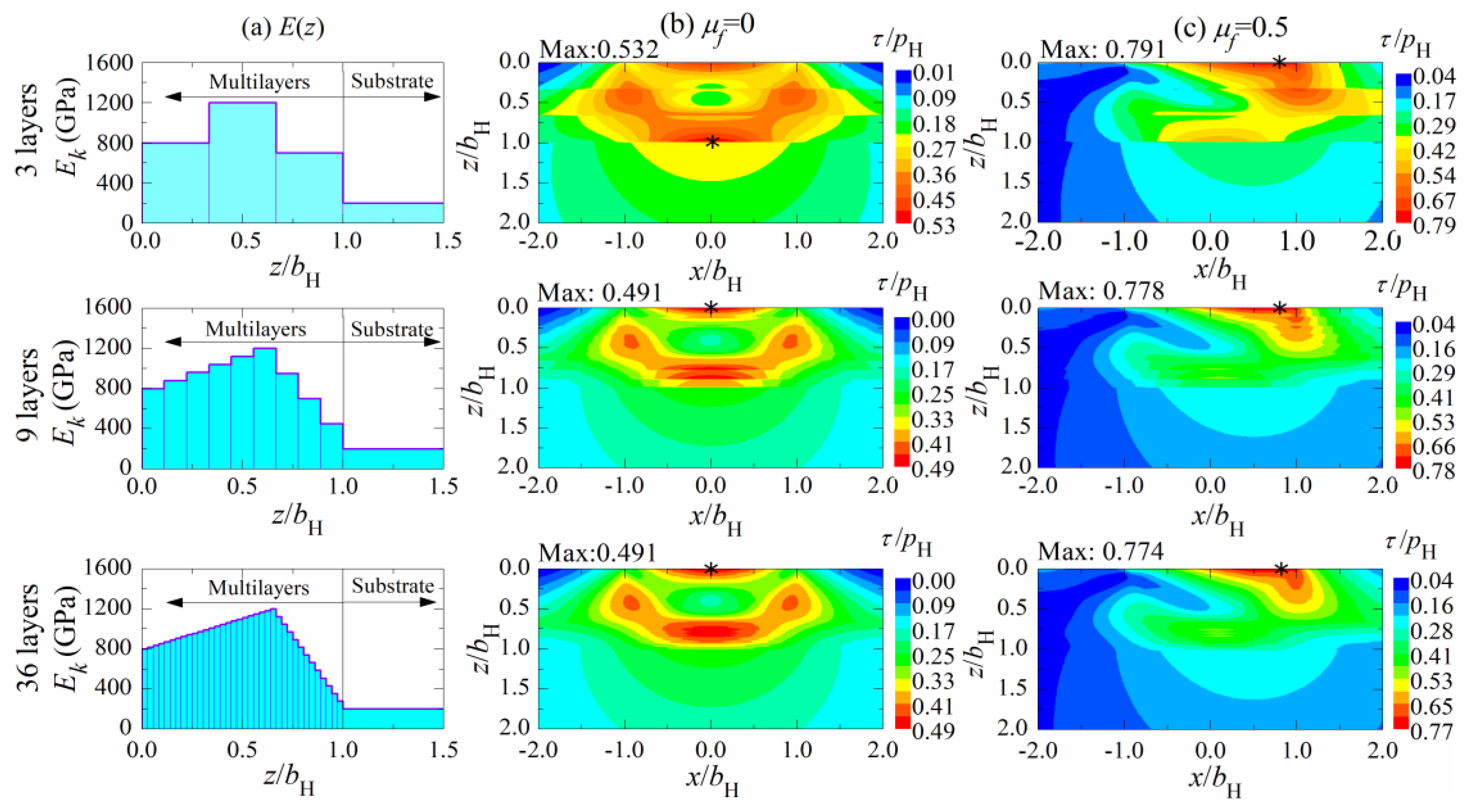
4.1. Influence of the Structure Layout of the Multilayers on the Mechanical Behavior

Figure 5 is the contour plots of the maximum shear stress in the subsurface of multilayered solids with various structure layouts when the friction coefficient is 0 and 0.5, respectively. The elasticity modulus along z axis of various structure layouts of the multilayers is shown in Figure 5a. The layer number N is 10, and all layers from the top layer to the bottom layer have the same thickness of b_H/10. The first layout of the multilayer is a monolayer coating since the elasticity modulus remains unchanged from the top layer to the bottom layer and changes abruptly on the interface between the bottom layer and the substrate. The other four layouts of the multilayers afford four alternatives to avoid the sudden change of elasticity modulus as that of the 1st layout through a gradient change layer by layer. For the first layout, a significant discontinuity can be found on the interface between the bottom layer and the substrate. The peak value of the maximum shear stress is 0.567p_H for μ_f = 0 and locates at the bottom of the bottom layer. This is a result of the sudden decrease of elasticity modulus on from 800 GPa of the layers to 200 GPa of the substrate. The peak value of the maximum shear stress increases rapidly to 0.816p_H for μ_f = 0.5 and its location shifts to the surface due to the friction traction applied on the surface. For the second layout, the significant discontinuity of the maximum shear stress as that of the 1st layout does not exist anymore and a relatively small discontinuity is observed on the interface of each two adjacent layers, and the discontinuity on the interface of the top five layers is more visible than that on the interface of the bottom five layers. The maximum shear stress decreases in the layers close to the substrate while increases dramatically in the surface region, so its peak value locates on the surface and reaches 0.582p_H for μ_f = 0 and 0.960p_H for μ_f = 0.5 respectively. For the third layout, the contour plots of the maximum shear stress are very similar to those of the second layout. The peak value of the maximum shear stress is 0.548p_H for μ_f = 0 and 0.886p_H for μ_f = 0.5 respectively and both locate on the surface of the multilayered solids. For the 4th layout, no discontinuity of the maximum shear stress is observed from the first layer to the fifth layer due to the same elasticity modulus of the top five layers. The maximum shear stress also reduces in the layers close to the substrate and increases in the surface region. The peak value of the maximum shear stress is 0.526p_H for μ_f = 0 and 0.836p_H for μ_f = 0.5 respectively and both locate on the surface too. For the fifth layout, the decrease of the maximum shear stress in the layers close to the substrate is not as significant as those of the second layout to fourth layout, and the increase of the maximum shear stress in the surface region is also not as significant as those of the second layout to fourth layout. The peak value of the maximum shear stress is 0.487p_H for μ_f = 0 and 0.764p_H for μ_f = 0.5 respectively, which are the smallest among the five layouts of the multilayers investigated numerically in this research.

Figure 6 shows the influence of the structure layouts of the multilayered solids on the peak value of the maximum shear stress under various friction coefficients. With the increase of the friction coefficient, the peak value of the maximum shear stress increases slightly when μ_f ranges from 0 to 0.2 for various layouts of multilayered solids, while increases relatively significantly when μ_f ranges from 0.2 to 0.5. For the second layout to fifth layout, the peak value of the maximum shear stress decreases in the order of the second layout, the third layout, the fourth layout and the fifth layout under various friction coefficients. As indicated in the figure, the peak value of the maximum shear stress of the second layout is larger than that of the first layout under various friction coefficients. The peak value of the maximum shear stress of the third layout and the fourth layout is smaller than that of the first layout when the friction coefficient is smaller than 0.1, and it is opposite when the friction coefficient is larger than about 0.2. It can be further observed that only the peak value of the maximum shear stress of the fifth layout is smaller than that of the first layout under various friction coefficients. Further, the peak value of the maximum shear stress of the fifth layout is about 16.3% smaller than that of the second layout when the friction coefficient is 0. Therefore, the peak value of the maximum shear stress, which is closely related to the yield and fatigue damage of materials [37,38], can be reduced effectively by optimizing the structure layout of multilayered solids and minimized by employing a structure layout with elasticity modulus increasing first in the top layers and then decreasing in the bottom layers just as the fifth layout shown in Figure 5a.

4.2. Influence of the Layer Number of the Multilayers on the Mechanical Behavior

Figure 7 is the contour plots of the maximum shear stress in the subsurface of multilayered solids with a similar structure layout of the multilayers but a different layer number. It can be seen from Figure 7b,c that the discontinuity of the maximum shear stress on the interface of each two adjacent layers becomes more invisible with the increase of the layer number for both μ_f = 0 and μ_f = 0.5, which is a result of that the difference in the elasticity moduli of each two neighboring layers becomes smaller with the increase of the layer number as shown in Figure 7a. The peak value of the maximum shear stress of the solid coated with three layers locates at the bottom of the third layer. However, it moves to the surface when the layer number increases to nine layers and 36 layers. A decrease of the peak value of the maximum shear stress can be observed when the layer number increases from three to nine, while almost no difference of the peak value of the maximum shear stress is observed when the layer number increases from 9 to 36.

The stress σ_xx along z axis of multilayered solids with a similar layout of the multilayers but a different layer number is shown in Figure 8 when the friction coefficient is 0. It can be observed that the stress σ_xx is discontinuous on the interface of each two neighboring layers, and the discontinuity of the stress σ_xx also becomes more invisible with the increase of the layer number. As indicated in Figure 7, the stress σ_xx is tensile in the region close to the substrate, and the tensile stress σ_xx is so large that its maximum value reaches up to 0.5p_H when the layer number is three. It also can be found that the maximum value of the tensile stress σ_xx in the region close to the substrate becomes smaller with the increase of the layer number, although the tensile stress σ_xx could not be completely eliminated by increasing the layer number. The maximum tensile stress σ_xx decreases to 0.28p_H when the layer number increases to 36. Obviously, the maximum tensile stress σ_xx, which is believed to be responsible for the initiation and propagation of cracks at the base of hard coatings [39,40], can be reduced effectively by increasing the layer number.

5. Conclusions

A semi-analytical method for the 2D mechanical behavior analysis of multilayered solids has been developed and validated in this paper. The influence of the structure layout and the layer number on the mechanical behavior of the multilayered solid has also been numerically investigated based on the present method. Several conclusions are drawn as follows:

• A 2D analytical frequency response functions of multilayered solids subjected to surface contact loading is derived and given in a recursive form.
• A 2D semi-analytical method for the mechanical behavior analysis of multilayered solids is developed by converting from its frequency response functions with an IFFT based numerical conversion method.
• Among various structure layouts numerically investigated in this paper, the layout with elasticity modulus increasing first in the top layers and then decreasing in the bottom layers can minimize the peak value of the maximum shear stress under various friction coefficients.
• The maximum tensile stress σ_xx in subsurface can be reduced effectively by increasing the layer number of multilayered solids.

References

1. Yang, D.K.; Wang, J.T.; Fabijanic, D.; Lu, J.Z.; Hodgson, P.D. Improved contact load-bearing capacity of ultra-fine grained titanium: Multilayering and grading. Mater. Des. 2014, 58, 217–225. [Google Scholar] [CrossRef]
2. Schulze, M.; Seidlitz, H.; Konig, F.; WeiB, S. Tribological investigations of PVD coated multi-layer constructions. J. Mater. Sci. Res. 2015, 5, 97–106. [Google Scholar] [CrossRef] [Green Version]
3. Huang, M.; Xu, C.; Fan, G.; Maawad, E.; Gan, W.; Geng, L.; Lin, F.; Tang, G.; Wu, H.; Du, Y.; et al. Role of layered structure in ductility improvement of layered Ti–Al metal composite. Acta Mater. 2018, 153, 235–249. [Google Scholar] [CrossRef]
4. He, D.; Li, X.; Pu, J.; Wang, L.; Zhang, G.; Lu, Z.; Li, W.; Xue, Q. Improving the mechanical and tribological properties of TiB 2/a-C nanomultilayers by structural optimization. Ceram. Int. 2018, 44, 3356–3363. [Google Scholar] [CrossRef]
5. Holmberg, K.; Matthews, A.; Ronkainen, H. Coatings tribology—Contact mechanisms and surface design. Tribol. Int. 1998, 31, 107–120. [Google Scholar] [CrossRef]
6. MohdTobi, A.L.; Shipway, P.H.; Leen, S.B. Finite element modelling of brittle fracture of thick coatings under normal and tangential loading. Tribol. Int. 2013, l58, 29–39. [Google Scholar] [CrossRef] [Green Version]
7. Csanadi, T.; Nemeth, D.; Lofaj, F. Mechanical properties of hard W–C coating on steel substrate deduced from nanoindentation and finite element modeling. Exp. Mech. 2017, 57, 1057–1069. [Google Scholar] [CrossRef]
8. Hossain, M.M.; Xiao, S.; Sue, H.; Kotaki, M. Scratch behavior of multilayer polymeric coating systems. Mater. Des. 2017, 128, 143–149. [Google Scholar] [CrossRef]
9. Kang, J.J.; Xu, B.S.; Wang, H.D.; Wang, C. Competing failure mechanism and life prediction of plasma sprayed composite ceramic coating in rolling–sliding contact condition. Tribol. Int. 2014, 73, 128–137. [Google Scholar] [CrossRef]
10. Luo, J.F.; Liu, Y.J.; Berger, E.J. Interfacial stress analysis for multi-coating systems using an advanced boundary element method. Comput. Mech. 2000, 24, 448–455. [Google Scholar] [CrossRef]
11. Zhang, Y.M.; Gu, Y.; Chen, J.T. Internal stress analysis for single and multilayered coating systems using the boundary element method. Eng. Anal. Bound. Elem. 2011, 35, 708–717. [Google Scholar] [CrossRef]
12. Xu, J.Q.; Mutoh, Y. Analytical solution for interface stresses due to concentrated surface force. Int. J. Mech. Sci. 2003, 45, 1877–1892. [Google Scholar] [CrossRef]
13. Xu, J.; Mutoh, Y. A normal force on the free surface of a coated material. J. Elast. 2003, 73, 147–164. [Google Scholar] [CrossRef]
14. Nie, C.; Zheng, D.; Gu, L.; Zhao, X.; Wang, L. Comparison of interface mechanics characteristics of DLC coating deposited on bearing steel and ceramics. Appl. Surf. Sci. 2014, 317, 188–197. [Google Scholar] [CrossRef]
15. Sneddon, I.N. Fourier Transforms; McGraw-Hill: New York, NY, USA, 1951. [Google Scholar]
16. Azhari, F.; Boroomand, B.; Shahbazi, M. Explicit relations for the solution of laminated plates modeled by a higher shear deformation theory: Derivation of exponential basis functions. Int. J. Mech. Sci. 2013, 77, 301–313. [Google Scholar] [CrossRef]
17. Shojaei, A.; Mossaiby, F.; Zaccariotto, M.; Galvanetto, U. A local collocation method to construct Dirichlet-type absorbing boundary conditions for transient scalar wave propagation problems. Comput. Methods Appl. Mech. Eng. 2019, 356, 629–651. [Google Scholar] [CrossRef]
18. Mossaiby, F.; Shojaei, A.; Boroomand, B.; Zaccariotto, M.; Galvanetto, U. Local Dirichlet-type absorbing boundary conditions for transient elastic wave propagation problems. Comput. Methods Appl. Mech. Eng. 2020, 362, 112856. [Google Scholar] [CrossRef]
19. Mejers, P. The contact problem of a rigid cylinder on an elastic layer. Appl. Sci. Res. 1968, 18, 353–383. [Google Scholar] [CrossRef]
20. Alblas, J.B.; Kuipers, M. On the two dimensional problem of a cylindrical stamp pressed into a thin elastic layer. Acta Mech. 1970, 9, 292–311. [Google Scholar] [CrossRef]
21. Gupta, P.K.; Walowit, J.A. Contact stresses between an elastic cylinder and a layered elastic solid. J. Lubr. Technol. 1974, 96, 250–257. [Google Scholar] [CrossRef]
22. King, R.B.; O’Sullivan, T.C. Sliding contact stresses in a two-dimensional layered elastic half-space. Int. J. Solids Struct. 1978, 23, 581–597. [Google Scholar] [CrossRef]
23. Wang, T.J.; Wang, L.Q.; Gu, L.; Zhao, X.L. Numerical analysis of elastic coated solids in line contact. J. Cent. South Univ. 2015, 22, 2470–2481. [Google Scholar] [CrossRef]
24. Elsharkawy, A.A.; Hamrock, B.J. A numerical solution for dry sliding line contact of multilayered elastic bodies. J. Tribol. 1993, 115, 237–245. [Google Scholar] [CrossRef]
25. Elsharkawy, A.A. Effect of friction on subsurface stresses in sliding line contact of multilayered elastic solids. Int. J. Solids Struct. 1999, 36, 3903–3915. [Google Scholar] [CrossRef]
26. Ke, L.L.; Wang, Y.S. Two-dimensional contact mechanics of functionally graded materials with arbitrary spatial variations of material properties. Int. J. Solids Struct. 2006, 43, 5779–5798. [Google Scholar] [CrossRef] [Green Version]
27. Ke, L.L.; Wang, Y.S. Two-dimensional sliding frictional contact of functionally graded materials. Eur. J. Mech. A-Solids 2007, 26, 171–188. [Google Scholar] [CrossRef]
28. Liu, J.; Ke, L.L.; Wang, Y.S. Two-dimensional thermoelastic contact problem of functionally graded materials involving frictional heating. Int. J. Solids Struct. 2011, 48, 2536–2548. [Google Scholar] [CrossRef] [Green Version]
29. Johnson, K.L. Contact Mechanics; Cambridge University Press: Cambridge, UK, 1985. [Google Scholar]
30. Erdilyi, A.; Magnus, W.; Oberhettinger, F.; Tricomi, F.G. Tables of Integral Transforms; Bateman Manuscript Project; McGraw-Hill: New York, NY, USA, 1954; Volume I. [Google Scholar]
31. Zaitsev, V.F.; Polyanin, A.D. Handbook of Exact Solutions for Ordinary Differential Equations; CRC Press: Boca Raton, FL, USA, 2002. [Google Scholar]
32. Zhang, J.J.; Wang, T.J.; Zhang, C.W.; Wang, L.Q.; Ma, X.X.; Yin, L.C.; Zhan, L.W.; Sun, D. A two-dimensional contact model between a multilayered solid and a rigid cylinder. Surf. Coat. Technol. 2019, 360, 382–390. [Google Scholar] [CrossRef]
33. Yu, C.; Wang, Z.; Wang, Q.J. Analytical frequency response functions for contact of multilayered materials. Mech. Mater. 2014, 76, 102–120. [Google Scholar] [CrossRef]
34. Liu, S.B.; Wang, Q. Studying contact stress fields caused by surface tractions with a discrete convolution and fast fourier transform algorithm. J. Tribol. 2000, 124, 36–45. [Google Scholar] [CrossRef] [Green Version]
35. Wang, T.J.; Ma, X.X.; Wang, L.Q.; Gu, L.; Yin, L.C.; Zhang, J.J.; Zhan, L.W.; Sun, D. Three-dimensional thermoelastic contact model of coated solids with frictional heat partition considered. Coatings 2018, 8, 470. [Google Scholar] [CrossRef] [Green Version]
36. McEwen, E. Stresses in elastic cylinders in contact along a generatrix. Philos. Mag. 1949, 40, 454–459. [Google Scholar]
37. Sadeghi, F.; Jalalahmadi, B.; Slack, T.S.; Raje, N.; Arakere, N.K. A Review of rolling contact fatigue. J. Tribol. 2009, 131, 041403. [Google Scholar] [CrossRef]
38. Walvekar, A.A.; Sadeghi, F. Rolling contact fatigue of case carburized steels. Int. J. Fatigue 2016, 95, 264–281. [Google Scholar] [CrossRef]
39. Piao, Z.Y.; Xu, B.S.; Wang, H.D.; Pu, C.H. Effects of thickness and elastic modulus on stress condition of fatigue-resistant coating under rolling contact. J. Cent. South Univ. Technol. 2010, 17, 899–905. [Google Scholar] [CrossRef]
40. Wang, T.J.; Wang, L.Q.; Gu, L.; Zheng, D. Stress analysis of elastic coated solids in point contact. Tribol. Int. 2015, 86, 52–61. [Google Scholar] [CrossRef]
Figure 1. Illustration of a half plane coated with multilayers subjected to surface contact loading.
Coatings 10 00429 g001
Figure 2. Comparison of the maximum shear stress of a half plane of the substrate material subjected to subjected to surface contact loading, (a) the exact analytical solution given by McEwen, (b) the solution of the present method.
Coatings 10 00429 g002
Figure 3. The illustration of the FEM model of the multilayered solid subjected to surface mechanical loading.
Coatings 10 00429 g003
Figure 4. Comparison of the maximum shear stress of a multilayered half plane with 40 layers subjected to surface contact loading, (a) the solution of FEM, (b) the solution of the present method.
Coatings 10 00429 g004
Figure 5. Contour plots of the maximum shear stress in the subsurface of multilayered solids with various structure layouts of multilayers, (a) the structure layouts of multilayers, (b) the contour plots of the maximum shear stress when μf = 0, (c) the maximum shear stress when μf = 0.5.
Coatings 10 00429 g005
Figure 6. Influence of the structure layout of multilayered solids on the peak value of the maximum shear stress in the subsurface under various friction coefficients.
Coatings 10 00429 g006
Figure 7. Contour plots of the maximum shear stress in the subsurface of multilayered solids with a similar structure layout but a different layer number, (a) the elasticity modulus along z axis, (b) the maximum shear stress when μf is 0, (c) the maximum shear stress when μf is 0.5.
Coatings 10 00429 g007
Figure 8. Stress σxx along z axis of multilayered solids with a similar structure layout but a different layer number when μf = 0.
Coatings 10 00429 g008