Article

Entropy Analysis of an MHD Synthetic Cilia Assisted Transport in a Microchannel Enclosure with Velocity and Thermal Slippage Effects

1
Department of Quantitative Methods, College of Business Administration, Imam Abdulrahman Bin Faisal University, P.O. Box 1982, Dammam 34212, Saudi Arabia
2
Department of Mathematics and Natural Sciences, Prince Mohammad Bin Fahd University, Khobar 31952, Saudi Arabia
*
Author to whom correspondence should be addressed.
Coatings 2020, 10(4), 414; https://doi.org/10.3390/coatings10040414
Submission received: 23 March 2020 / Revised: 13 April 2020 / Accepted: 20 April 2020 / Published: 22 April 2020

Abstract

:
The magnitude of shear stress at the ciliated wall is considered as the measure of efficiency of cilia beatings as it describes the momentum transfer between the medium and the cilia. Under high shear rate, some non-Newtonian fluids behave as visco-inelastic fluids. We consider here a ciliated channel coated with Prandtl fluid, a visco-inelastic fluid, with Hartmann layer under momentum and thermal slip effects. The flow in the channel is produced due to beatings of cilia that obey an elliptic path of motion in the flow direction. An entropy analysis of the flow is also conducted in wave frame. After introducing lubrication approximations in the governing equation, the perturbation solutions are calculated. The data for pressure rise per metachronal wavelength and frictional force at the ciliated wall are obtained by numerical integration. The analysis reveals that the higher values of cilia length and velocity slip parameters support fluid flow near the channel wall surface. Fluid temperature is an increasing function of thermal slip but a decreasing function of cilia length and slip parameters. Entropy in the channel can be minimized with an increase in cilia length and slip effect at the boundary. The magnitude of the heat transfer coefficient decreases by taking the substantial slippage and tiny cilia in length at the microchannel wall.

1. Introduction

Cilia-aided movements are considered as an important factor for the locomotion of the cell itself or other substances past the cell surface. Cilia are very tiny hair-resembling structures that develop from the outer surface of eukaryotic cells. They behave like oars, whipping back and forth in unison to produce a rhythmic pattern of waves travelling along the surface. Motile cilia in the respiratory system [1,2] are responsible for generating fluid flow on the cell surface to removes mucus and dust to make airways clean. In the digestive tract [3], cilia carry food and its egestion. Cilia coating in female fallopian tubes [4,5] carry the ova through oviducts, and in male efferent ductules [6] mix sperms to prevent them from accumulating and obstructing the tube so they can reach their final destination. They are also found in brain, kidneys, ears and eye retina. Due to its diverse applications in bioengineering and physiological disciplines, it has become an appealing field of research [7,8,9]. An interesting study dealing with the motion of microorganisms in non-Newtonian fluid induced by cilia and flagella have presented by Qiu et al. [10]. Brennen [11] have examined the movement of cell through viscous fluid stimulated by a harmonic wave travelling along the surface. Wu et al. [12] have studied the hydrodynamic ciliary pumping transport of Carreau fluid under lubrication assumptions. Farooq and Siddiqui [13] have reported that the cilia-driven flow of couple stress fluid was generated due to metachronal waves. Farooq et al. [14] have discussed the ciliary pumping transport of micropolar fluid inside a tube by considering long wavelength and low Reynolds number assumptions.
The study of biorheological fluids in the presence of electric and magnetic environment has tremendous applications in physiology, bioengineering and physics. For instance, magnetic field characteristics are used in the formation of magnetic devices, controlling the fluid temperature, blood reduction during surgeries, blood plasma, hyperthermia treatment, tumor cancer treatment and thermal insulation, etc. Stud et al. [15] have attempted the hydromagnetic peristaltic transport of physiological fluid in channel and reported that magnetic field resists the fluid flow. Mekheimer [16] have stated the effects of transverse magnetic field in a non-uniform symmetric channel filled with couple stress fluid. The flow of micropolar fluid under the effects of external magnetic field was studied by Hatzikonstantinou and Vafeas [17]. Tripathi [18] has presented a mathematical model of magnetohydrodynamic blood flow in a wavy channel under wavelength and small Reynolds. Some recent studies incorporating the impact of magnetic field in biological fluid flows are reported [19,20,21,22].
Flows that generate significant variations in velocity over small distances under a high shear rate induce a drop in fluid viscosity. When mucus, accepted as a non-Newtonian fluid, undergoes a rapid shear rate, a slippage layer is developed to act as a lubricant between the moving surfaces. Consequently, velocity slip plays a key role in the reduction in resistance to fluid flow. In microdevices and thin films, no-slip conditions for motion and energy conservation are not applicable. The existence of momentum and thermal slippage finds uses in mucociliary clearance, micro viscous pumps, drug delivery systems, microelectronic cooling, polymer and fuel cell, etc. Some relevant studies revealing the importance of slip condition are cited in [23,24,25,26,27].
Spontaneous chemical reactions that take place in biological systems are always accomplished by a drop in free energy. For example, metabolism in living organisms involving a series of chemical reactions generates free energy and is accompanied with substantial level entropy production. Usually in biological systems, antientropic processes such as muscle contractions, the dynamic flow of substances (urination, perspiration and blood flow, etc.) and biosynthesis are considered as entropy compensates. Due to its significant role in biology and industry, the entropy analysis of biological flows has become an appealing and mounting area of research [28,29,30,31] in recent years. The pioneer work demonstrating the entropy production in four different heat convective processes and entropy generation minimization was reported by Bejan [32,33]. Souidi et al. [34] presented the mathematical analysis of entropy generation in biological fluid flow. Later on, Akbar [35] extended the work by incorporating the effects of magnetic field in a wavy channel. Saleem [36] and Munawar et al. [37] have conducted the entropy analysis in peristaltic flows of variable viscosity fluid in symmetric and asymmetric channels. Recently, Saleem and Munawar [38] investigated the entropy generation in the ciliary flow of biomagnetic fluid.
Inspired by the aforementioned bulk of the literature, the main purpose of this study is to investigate the entropy generation in magnetohydrodynamic cilia-driven transport of Prandtl fluid by imposing the momentum slip and temperature jump conditions at the ciliated wall of the channel. The entire study is conducted in wave frame under realistic lubrication assumptions. The governing equations are solved using the regular perturbation method. Numerical integration is performed to calculate pressure rise per metachronal wavelength and frictional forces at the ciliated boundary. A detailed graphical analysis is made for axial velocity and temperature profiles, pressure gradient, stream function, total entropy generation number, the Bejan number and heat transfer coefficient in the results and discussion section of the manuscript.

2. Mathematical Formulation

Consider the two-dimensional pumping transport of non-Newtonian Prandtl fluid in a symmetric channel with artificial cilia spread uniformly along the channel wall. Heat convection in the fluid starts due the heated wall of the channel at a fixed temperature T1. It is supposed that a constant magnetic field B0 is imposed in the normal direction of the fluid motion. Furthermore, it is also assumed that the electric current in the channel is generated due to metachronal waves of cilia moving with constant speed c along with the channel wall. In a rectangular coordinate system, we assume the X ¯ -axis along the direction of metachronal wave propagation and Y ¯ -axis perpendicular to it. The schematic diagram (Figure 1) shows the flow and heat transfer configuration of the problem. The structure of the ciliated at the wall is described by the following function:
Y ¯ = f ( X ¯ , t ) = H = [ a + a ε   c o s ( 2 π λ ( X ¯ c t ) ) ] .
It is supposed that cilia tips whipped by accomplishing elliptic motion and are vertically situated at
X ¯ = g ( X ¯ , t ) = X 0 + a ε α   s i n ( 2 π λ ( X ¯ c t ) ) ,
where a, α, ε, H, t, λ and X0 are the mean width of the ciliated channel, measure of the eccentricity, cilia length parameter, half channel width, time, wavelength of metachronal wave and specified position of the fluid particle.
The cilia move with the following axial and transverse velocities in the fixed frame [39,40]:
U ¯ 0 = ( X ¯ t ) X 0 = ( 2 π λ ) a c ε α   c o s ( 2 π λ ( X ¯ c t ) ) 1 ( 2 π λ ) a ε α   c o s ( 2 π λ ( X ¯ c t ) )   ,
V 0 ¯ = ( Y ¯ t ) X 0 = ( 2 π λ ) a c ε α   s i n ( 2 π λ ( X ¯ c t ) ) 1 ( 2 π λ ) a ε α   s i n ( 2 π λ ( X ¯ c t ) ) .
The basic laws of mass, momentum and energy are given by the following equations
· V = 0 ,
ρ dV dt = P ¯ + · S + J × B ,
ρ C P d T ¯ d t = κ 2 T ¯ + S . V ,
where V = ( U ¯ , V ¯ , 0 ) is the velocity vector, J = σ (E + V × B) is current density and B = B0 + B1 is the total magnetic field that appears as the sum of constant (B0) and induced (B1) magnetic fields. We assume that B0 is applied in the normal direction of flow. Therefore, under the assumption of small magnetic Reynolds and in the absence of electric field effects, the Lorentz force reduces to   J × B = σ B 0 2   ( U ¯ , 0 , 0 ) .
In the fixed frame of reference, the resulting governing equations for two-dimensional flow are given by
U ¯ X ¯ + V ¯ Y ¯ = 0   ,
ρ ( t + U ¯ X ¯ + V ¯ Y ¯ ) U ¯ = P ¯ X ¯ + S X X X ¯ + S X Y Y ¯ σ B 0 2 U ¯ ,
ρ ( t + U ¯ X ¯ + V ¯ Y ¯ ) V ¯ = P ¯ Y ¯ + S X Y X ¯ + S Y Y Y ¯ σ B 0 2 V ,
ρ C P ( T ¯ t + U ¯ T ¯ X ¯ + V ¯ T ¯ Y ¯ ) = κ ( 2 T ¯ X ¯ 2 + 2 T ¯ Y ¯ 2 ) + S X X U ¯ X ¯ + S X Y ( U ¯ Y ¯ + V ¯ X ¯ ) + S Y Y V ¯ Y ¯   ,
where SXX, SXY and SYY are the components of the stress tensor for the Prandtl fluid, ρ is the fluid density, σ the electrical conductivity, P ¯ the fluid pressure and ( U ¯ , V ¯ ) are the velocity components in ( X ¯ , Y ¯ ) directions, Cp the specific heat, κ the thermal conductivity and T ¯ the fluid temperature.
To transform the laboratory frame into wave frame, the following relations are used:
x ¯ = X ¯ c t ,   y ¯ = Y ¯ ,   u ¯ = U ¯ c ,   v ¯ = V ¯ ,   p ¯ ( x , y ) = P ¯ ( X ¯ , Y ¯ , t ) .
Introducing the following non-dimensional quantities
x = x ¯ λ ,   y = y ¯ a ,   u = u ¯ c ,   v = λ v ¯ a c ,   θ = T T 0 T 1 T 0 ,   H = H ¯ a ,   t = c t ¯ a ,   p = a 2 p ¯ μ c λ ,   β = a λ ,   η = μ A C , ϕ = η c 2 C 2 a 2 ,   s = a S μ c , Re = a c ν ,   M 2 = σ B 0 2 a 2 μ ,   Pr = μ C P κ , E c = c 2 C P ( T 1 T 0 ) ,   B r = E c P r .
Using Equations (7) and (8), Equations (3)–(6) take the following forms
β ( u x + v y ) = 0 ,
R e   β ( u u x + v u y ) = p x β 2 s x x x s x y y M 2 ( u + 1 ) ,
R e   β 3 ( u v x + v v y ) = p y β 3 s x y x β s y y y ,
R e   β ( u θ x + v θ y ) = 1 P r ( β 2 2 θ x 2 + 2 θ y 2 ) + E c β [ s x x u x + s x y ( v x + 1 β u y ) + s y y v y ] ,
where p is the fluid pressure, (u, v) are the dimensionless velocity components in (x, y) directions, Re the Reynolds number, M the Hartmann number, β the wave number, η the fluid material parameter, ϕ the time relaxation parameter, Pr the Prandtl number, Ec the Eckert number, Br the Brinkman number and θ is the fluid temperature. The existing component of the stress tensor for the Prandtl fluid are defined as [41,42]
S X Y = [ A μ s i n 1 [ 1 C { ( U ¯ Y ¯ ) 2 ( V ¯ X ¯ ) 2 } 1 / 2 ]   { ( U ¯ Y ¯ ) 2 ( V ¯ X ¯ ) 2 } 1 / 2 ] U ¯ Y ¯ ,
where the function sine inverse is expanded up to first two terms only, since the rest of the terms are negligible. Using the lubrication approximation that the metachronal wavelength is very long (β ≪ 1), and insignificant inertia (Re→0), the resulting equations Equations (9)–(12) adopt the following form:
p x = y { η ( u y ) + ϕ 6 ( u y ) 3 } M 2 ( u + 1 ) ,
p y = 0 ,
2 θ y 2 = B r [ η ( u y ) 2 + ϕ 6 ( u y ) 4 ]
The corresponding nondimensional boundary conditions imposed on flow problem are listed as
u y = 0 , θ y = 0   at   y = 0 ,
u + ξ [ η u y + ϕ 6 ( u y ) 3 ] = 1 2 π α ε β   c o s ( 2 π x ) 1 2 π α ε β   c o s ( 2 π x ) , θ + Ω θ y = 1 , } a t   y = h = 1 + ε   c o s ( 2 π x ) ,
where ξ , Ω and h are dimensionless forms of velocity slip parameter, thermal slip parameter and ciliated wall. The pressure-rise per wavelength ΔP, the fluid frictional force (ΔFλ) and heat transfer coefficient Z (at the ciliated channel wall) are expressed as [43,44,45]:
Δ P = 0 1 ( d p d x ) d x ,
Δ F λ = 0 1 h ( x ) ( d p d x ) d x ,
Z = h x θ y .
The nondimensional mean flow rate in the laboratory frame (Q) and in the wave frame (F) are described by
F = 0 h u d y , Q = F + 1 .

3. Perturbation Solution

In order to solve Equations (14)–(16) subject to the boundary conditions (17) and (18), we use a regular perturbation method assuming ϕ (<<1) as the perturbation parameter. Expanding the dependent variables by Taylor’s Series expansion, one gets
u = u 0 + ϕ u 1 + O ( ϕ 2 ) ,
d p d x = d p 0 d x + ϕ d p 1 d x + O ( ϕ 2 ) ,
F = F 0 + ϕ F 1 + O ( ϕ 2 ) ,
θ = θ 0 + ϕ θ 1 + O ( ϕ 2 ) .
Using the above series in Equations (14)–(18), we obtained the zeroth and first order system of linear differential equations.

3.1. Zeroth Order System

d p 0 d x = η 2 u 0 y 2 M 2 ( u 0 + 1 ) ,
2 θ 0 y 2 = B r η ( u 0 y ) 2 ,
F 0 = 0 h u 0 d y .
The corresponding boundary conditions are
u 0 y = 0 ,       θ 0 y = 0   at   y = 0 ,
u 0 + ξ η u 0 y = 1 2 π α ε β   c o s ( 2 π x ) 1 2 π α ε β   c o s ( 2 π x ) , θ 0 + Ω θ 0 y = 1 , } at   y = h = 1 + ε   c o s ( 2 π x ) .

3.2. First Order System

d p 1 d x = η 2 u 1 y 2 M 2 u 1 + ϕ 6 y ( u 0 y ) 3 ,
2 θ 1 y 2 = B r [ η ( u 0 y ) 2 + 1 6 ( u 0 y ) 4 + η ( u 1 y ) 2 + 2 η u 0 y u 1 y ] ,
F 1 = 0 h u 1 d y .
The corresponding boundary conditions are
u 1 y = 0 , θ 1 y = 0   at   y = 0 ,
u 1 + ξ [ η u 1 y + 1 6 ( u 0 y ) 3 ] = 0 , θ 1 + Ω θ 1 y = 0   at   y = h = 1 + ε   c o s ( 2 π x ) .
After solving zeroth and first order system of equations, the explicit form solutions for the axial velocity, the pressure gradient and the temperature are obtained as
u ( y ) = h M c o s h ( y A 8 ) + η A 5 + M Q A 1 ( c o s h ( y A 8 ) + A 11 ) A 1 A 17 + A 16 M 5 ϕ ( h + Q A 1 ) 3 32 A 11 A 1 3 η 5 / 2 A 17 3 ,
d p d x = M 7 ϕ ( h + Q A 1 ) 3 [ 12 M h + 9 η ξ M 12 M η ξ   c o s h ( 2 A 2 ) + 3 M η ξ   c o s h ( 4 A 2 ) + η A 10 ] 32 η 2 A 1 3 A 17 3 A 9 A 11 + M 2 ( M ( h Q ) A 1 A 4 + η ( M 2 ( h Q ) ξ + 2 π α β ε ( 1 + M 2 ξ ( h + Q ) ) c o s ( 2 π x ) ) A 5 ) A 1 A 17 ,
θ = A 32 8 A 29 2 + M 6 ϕ B r A 23 A 40 ( 1800 η A 19 A 24 A 23 3 + A 29 ( 300 η A 23 3 ( 16 A 4 A 25 + η A 41 ) A 31 ( 3600 η A 4 ( 3 η + 2 M 2 A 26 ) + 75 η A 6 A 27 + A 36 + A 37 + A 38 + A 39 + A 42 ) ) ) ,
where
A 1 = 1 + 2 π α β ε   c o s ( 2 π x ) ,   A 2 = h M η ,   A 3 = 1 + h M 2 ξ ,
A 4 = c o s h ( A 2 ) ,   A 5 = s i n h ( A 2 ) ,   A 6 = c o s h ( 3 A 2 ) ,   A 7 = s i n h ( 3 A 2 ) ,
A 8 = M η ,   A 9 = h M + η M ξ η + cot h ( A 2 ) ,
A 10 = 8 s i n h ( 2 A 2 ) + s i n h ( 4 A 2 ) ,   A 11 = A 4 + M ξ η A 5 ,
A 12 = 4 h M 2 ξ η   c o s h ( y A 8 ) + η   c o s h ( 3 y A 8 ) 4 M y s i n h ( y A 8 ) ,
A 13 = 12 h M + 9 M ξ η 12 M ξ η   c o s h ( 2 A 2 ) + 3 M ξ η   c o s h ( 4 A 2 ) 8 η   s i n h ( 2 A 2 ) + η   s i n h ( 4 A 2 ) ,
A 14 = 4 ( h + η ξ ) c o s h ( y A 8 ) + η ξ   c o s h ( 3 y A 8 ) 4 M y η ξ   s i n h ( y A 8 ) ,
A 15 = 32 s i n h 3 ( y A 8 ) 9 A 7 ,
A 16 = 3 A 6 η   c o s h ( y A 8 ) + 3 A 4 A 12 + η A 13 ( c o s h ( y A 8 ) + A 11 ) A 17 + M ( 3 A 5 A 14 + η ξ A 15 c o s h ( y A 8 ) ,
A 17 = h M A 4 + η A 3 A 5 ,   A 18 = B r ( 1 2 π α β ε   c o s ( 2 π x ) ) 2 ,   A 19 = 3 M ξ η   c o s ( 4 A 2 ) + η A 10 ,
A 20 = 2 h 2 B r Q 2 M 2 ( h 2 y 2 + 2 h Ω ) + 4 h η ξ 2 M 2 h 2 η ξ 2 + h 2 M 2 ( y 2 h 2 2 h Ω ) A 18 A 44 ,
A 21 = η 5 2 A 1 4 ( A 4 + M ξ η A 5 ) ( h M A 4 + η A 3 A 5 ) 5 ,
A 22 = 4 η + M 2 ( B r Q 2 η + h ( 8 η ξ + h ( 4 + 4 M 2 η ξ 2 + η A 18 + 2 B r Q η A 1 ,  
A 23 = h + Q 2 π Q α β ε   c o s ( 2 π x ) ,
A 24 = η   c o s h ( 2 A 2 ) + η   c o s h ( 2 y A 8 ) + 2 M ( M ( h 2 y 2 + 2 h Ω ) η Ω   s i n h ( 2 A 2 ) ) ,
A 25 = η + M 2 ( 3 h 2 3 y 2 + 6 h Ω + 2 η ξ Ω ) ,
A 26 = 6 y 2 6 h 3 M 2 η ξ Ω + 3 h ( 2 M 2 y 2 ξ + η ξ + 2 Ω ) + h 2 ( 6 12 M 2 ξ Ω ) ,
A 27 = 81 η 4 M 2 A 30 ,
A 28 = 2 η + M η   s i n h ( 2 A 2 ) ( B M 2 Q 2 Ω + h ( 4 + 2 M 2 B r η Ω A 1 ) + h 2 M 2 ( 4 ξ + Ω A 18 ) ) + M 2 A 20 ,
A 29 = h M A 4 + η A 3 A 5 ,   A 30 = ( 36 h 2 36 y 2 + 72 h Ω 301 η ξ Ω ) ,   A 31 = 1 + 4 M 2 Ω ξ ,
A 32 = M 2 η A 23 2 c o s h ( 2 y A 8 ) A 18 + c o s h ( 2 A 2 ) A 22 + 2 A 28 ,
A 33 = η A 31 c o s h ( 5 A 2 ) η ( c o s h ( ( h 4 y ) A 8 ) + c o s h ( ( h 4 y ) A 8 ) ) + 16 η ( c o s h ( ( h 2 y ) A 8 ) + c o s h ( ( h + 2 y ) A 8 ) ) ,
A 34 = M s i n h ( 5 A 2 ) ( ξ η + 4 Q ) + M ξ η ( s i n h ( ( h 4 y ) A 8 ) + s i n h ( ( h 2 y ) A 8 ) + s i n h ( ( h + 4 y y ) A 8 ) ) ,
A 35 = 48 M 3 ( h 2 y 2 ) ξ A 5 + 16 M η ξ A 5 32 M Ω A 5 + 96 M 3 Ω ξ A 5 ,
A 36 = 61,440 M 2 η 3 / 2 ξ ( h y Q ) + 675 η 3 / 2 c o s h ( 5 A 2 ) 14,940 M 2 η 3 / 2 ξ Ω   c o s h ( 5 A 2 ) + 2025 η 3 / 2 c o s h ( ( h 4 y ) A 8 ) 1800 η 3 / 2 c o s h ( ( h 2 y ) A 8 ) ,
A 37 = 10,800 M 2 η 3 / 2 ξ   c o s h ( ( h 2 y ) A 8 ) ( h y ) 2700 η 3 / 2 c o s h ( ( 3 h 2 y ) A 8 ) η 3 / 2 c o s h ( ( h + 2 y ) A 8 ) ( 8100 10,800 h ξ M 2 ) ,
A 38 = 10,800 M η   s i n h ( ( h 2 y ) A 8 ) + 10,800 ( M y η 2 S i n h ( ( h 2 y ) A 8 ) 3 η 2 ξ M S i n h ( ( 3 h 2 y ) A 8 ) ) + 115,200 S i n h ( y A 8 ) ,
A 39 = 2025 M η 2 ξ   s i n h ( ( h + 4 y ) A 8 ) + 400 h M A 5 ( 54 η 216 η ξ + 216 μ ξ Ω h ) 32,400 M 3 ξ η A 7 ( h 2 y 2 ) + 25 M η ξ A 7 ( 997 η + 756 Ω 2592 M 2 Ω ) ,
A 40 = 1 460,800 η 5 2 A 1 4 ( A 4 + M η ξ A 5 ) A 29 5 ,
A 41 = 3 η A 6 ( 5 + 12 M 2 Ω ξ ) 17 M η ξ A 7 28 M Ω A 7 + A 33 + A 34 + A 35 ,
A 42 = 675 η 3 2 ( 16 M 2 y c o s h ( ( h + 2 y ) A 8 ) 4 c o s h ( ( 3 h + 2 y ) A 8 ) + 3 c o s h ( ( h + 4 y ) A 8 ) ) + 9 M η   s i n h ( 5 A 2 ) ( 163 η ξ 300 Ω ) + 25 M η 2 ξ ( 81   s i n h ( ( h 4 y ) A 8 ) 1024   s i n h ( 3 y A 8 ) + 4608 25 s i n h ( 5 A 8 ) ) + 10,800 M η   s i n h ( ( h + 2 y ) A 8 ) ( h y ) + 2700 M η 2 ξ ( s i n h ( ( h + 2 y ) A 8 ) 3   s i n h ( ( 3 h + 2 y ) A 8 ) ) ,
We have calculated the pressure-rise per metachronal wavelength and the fluid frictional force by numerical integration of Equations (24) and (25).
To validate the above first-order perturbation solution, we made a comparison with previously reported results by with Jothi et al. [46] considering a limiting case (for non-ciliated channel and ξ→0) In Figure 2, we compare the velocity profiles of both studies on the same scale of axes. The figure shows a good agreement between both solutions, which indicates that the first-order perturbation series provides enough accuracy and thus verifies the efficiency of the present solution.

4. Entropy Analysis

We assume two main causes of entropy production: the heat transfer irreversibility and the fluid friction irreversibility. Thus, the total volumetric local rate of entropy generation is described by [47,48]
S g e n ''' = k T 0 2 ( T ) 2 + μ 0 T 0 [ S · V ] .
Dividing Equation (45) with the characteristic entropy (SG0) and using Equations (14) and the lubrication approximations in, one gets the total entropy generation number (NG) as:
N G = τ ( θ y ) 2 + B r { η ( u y ) 2 + ϕ 6 ( u y ) 4 } ,
where τ = ∆T/T0 is the nondimensional temperature difference (assuming τ = 1). In Equation (46), the first term signifies the entropy due to heat transfer while the second term associated with the Brinkman number corresponds to the fluid friction irreversibility.
Introducing the Bejan number to enquire the discerning effects of fluid friction irreversibility over the heat transfer irreversibility
B e = 1 1 + Φ ,
where Φ = B r { η ( u y ) 2 + ϕ 6 ( u y ) 4 } / τ ( θ y ) 2 represents the ratio of fluid friction irreversibility to the heat transfer irreversibility. The Bejan number Be takes the values between 0 and 1. Its value of more than 0.5 implies the leading effects of heat transfer irreversibility over fluid friction irreversibility and its value of less than 0.5 directs that dominating effects of fluid friction irreversibility.

5. Results and Discussion

In this section, a graphical analysis is presented for the various important physical quantities, such as axial velocity u(y), pressure gradient dp/dx, pressure-rise per wavelength ∆P, fluid frictional force Fλ at the ciliated wall, the total entropy generation number Ng, and the Bejan number Be, and streamlines by varying the different parameters of interest. Figure 3, Figure 4, Figure 5 and Figure 6 determine the effects of velocity slip parameter (ξ), cilia length (ε), Prandtl fluid (η) and time relaxation parameters (ϕ) on the velocity profile. From Figure 3, it can be seen that the axial velocity is impeded with increasing ξ in the channel center. At the channel wall, the fluid velocity is no longer equal to the velocity of the boundary due to the occurrence of slip. Therefore, at the boundary the fluid velocity augments as ξ increases. Figure 4 indicates that large values of ε create more resistance at the center of the channel, which causes deceleration in the fluid velocity. However, near the edge of the channel, the axial velocity augments by increasing ε. Figure 5 shows the velocity profile against various values of time relaxation parameter ϕ. It is observed from the figure that the velocity profile increases near the center part of the channel as ϕ increases. However, an inverse behavior is noticed close to the boundary. This is because of the decreasing strain rate as ϕ increases which results in a decrease in velocity near the boundary. Figure 6 states that at lesser values of fluid material parameter η, the velocity profile enhances near the channel wall and decreases at the center. This behavior of Prandtl fluid parameters is quite expected as increasing η corresponds to a high shear rate which results in a large velocity near the wall.
Figure 7 reveals that the adverse pressure gradient is boosted for higher values of cilia length parameter ε, and this increase is more significant in the contracted channel part. From Figure 8, the adverse pressure gradient decreases as the velocity slip parameter ξ increases. This reduction is more noticeable in the contracted channel part than the channel wider part. Figure 9 depicts that the adverse pressure gradient noticeably increases as the material parameter η increases and this increases is more significant in the contracted part of the channel as compared to the wider part. From Figure 10, it is observed that higher values of cilia length parameter ε enhance the pressure rise in the pumping zone but produce a decline in the augmented pumping zone. Figure 11 and Figure 12 illustrate that the pressure rise per metachronal wavelength increases with a decrease in slip parameter ξ and Prandtl fluid parameter η in the pumping zone. The effect of these parameters is completely converse in the augmented pumping zone. Moreover, the effects of ε, ξ and η are insignificant in the free pumping zone.
From Figure 13, it is noticed that the fluid temperature cools down by increasing the slip parameter ξ. This decrease is more prominent at the channel center as compared to the wall. This is due to the decrease in the convective heat transfer effect because of the jump in the fluid velocity at the boundary. Figure 14 shows that the fluid temperature rises when large values of thermal slip parameter Ω are taken into consideration. This is obvious since the fluid temperature is higher than the boundary temperature, and increasing the thermal slip parameter results in low convection near the boundary. Figure 15 and Figure 16 reveal that large values of cilia length parameter ε and the Hartmann number M induce a noticeable drop in the fluid temperature near. Since both resist the fluid flow and reduce the convection phenomenon in the flow, this drop in temperature is obvious.
Figure 17 indicates that the total entropy generation number decreases as the cilia length ε increases. Moreover, the cilia length parameter helps in promoting fluid friction irreversibility and demoting the heat transfer irreversibility (see, for instance, Figure 18). Figure 19 demonstrates that the total entropy increases as the fluid material parameter η increases. This increase is more significant at the channel wall which is due to the high viscous effects near channel boundary. From Figure 20, it can be seen that the entropy of the ciliated channel rises with an increase in eccentricity parameter α. Figure 21 shows that the velocity slip parameter also reduces the entropy production in the channel and this reduction is due to a decrease in the heat transfer irreversibility and the dominancy of fluid friction irreversibility, as observed from Figure 22. In Figure 23 and Figure 24, 3D visualizations of the total entropy generation number and the Bejan number, respectively, are presented. Figure 23 discloses that the total entropy generation number is at its maximum in the narrow part of the channel, while in the wider part it has lower values. This indicates that the entropy increases due to the compression of the channel. The dominancy of the irreversibilities can be analyzed through Figure 24, where the Bejan number is plotted against x and y variables. It indicates that at the narrow part of the channel, the effect of the irreversibility due to heat transfer is dominated, however, in the wider part of the channel heat transfer irreversibility decreases and the fluid friction irreversibility starts increasing.
From Figure 25 and Figure 26, the graphs of the heat transfer coefficient are found to be oscillating in shape. This behavior is quite likely due to metachronal waves travelling along the channel wall (stimulated by the power and recovery strokes of evenly distributed cilia lined in the channel surface). It is observed that the heat transfer coefficient decreases in magnitude when higher values of slip parameter ξ and small values of cilia length ε are selected. To see the effects of frictional force at the ciliated wall versus mean flow rate, Figure 27, Figure 28 and Figure 29 are presented. It is noticed that the behavior of frictional forces at the ciliated wavy wall is entirely opposite to pressure rise per metachronal wavelength. A direct proportionality between the frictional force and mean flow rate can be exhibited through Figure 27 and Figure 28. Figure 27 indicates that the frictional force is a decreasing function of Hartmann number in region 4 < Q < 2 and an increasing function in region 2 < Q < 8 . From Figure 28, it is clear that the cilia reduce frictional forces at the wall in region 2 < Q < 1 but support the frictional forces in the region 1 < Q < 4. Figure 29 depicts that the zone 2 < Q < 2 , the higher values of velocity slip parameter enhance the frictional force effects. However, in the 2 < Q < 4 part, frictional force decreases as the situation is moved from non-slip to partial slip.
Trapping is a remarkable manifestation of pumping ciliary flow. The development of internally circulating fluid mass confined by streamlines of travelling waves in wave frame is named as trapping. Due to an elevated flow rate and substantial occlusions, confined bolus is carried by streamlines and driven forward along with the metachronal wave (by power and recovery strokes of cilia). From Figure 30, it is established that the imprisoned bolus enlarges in size for large values of cilia length ε which indicates the increasing flow rate. Figure 31 demonstrates the effects of velocity slip parameter ξ on streamlines. The graph shows that the flow rate decreases as the velocity slip increases. Figure 32 depicts that the size of the trapped bolus shrinks down as the Hartmann number M increases. This indicates the reduction in the flow rate, which is due to the increase in the resistive Lorentz force against the flow.

6. Conclusions

A complete thermodynamical analysis has been presented for a ciliated channel coated with a visco-inelastic Prandtl fluid under the uniform magnetic field in wave frame. The effects of momentum slippage and temperature jump are considered at the boundary of a symmetric channel. The flow in the channel is induced due to the propagation of metachronal waves produced by cilia motion. Assuming a long wavelength and low Reynolds number approximations, the governing equations are normalized and solved with a regular perturbation method. Some important remarks extracted from the study are:
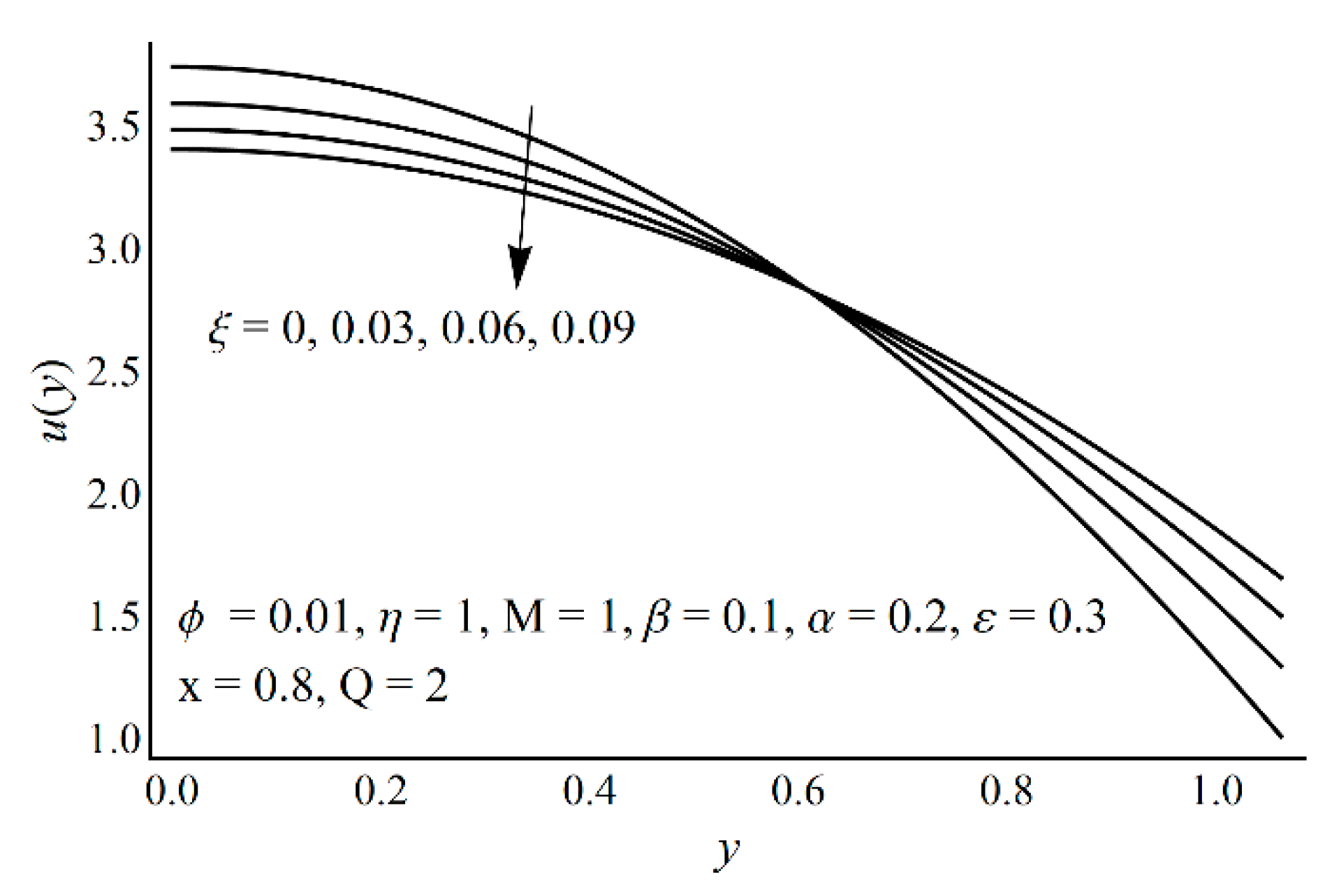
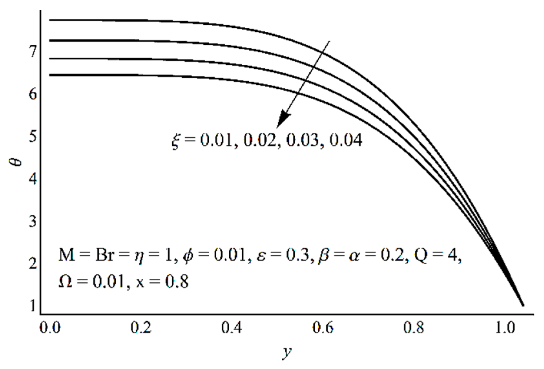
  • As the cilia length increases, the temperature profile and the entropy production decrease, while the velocity profile shows the opposite effect near the boundary and demonstrates decreasing effects near the center;
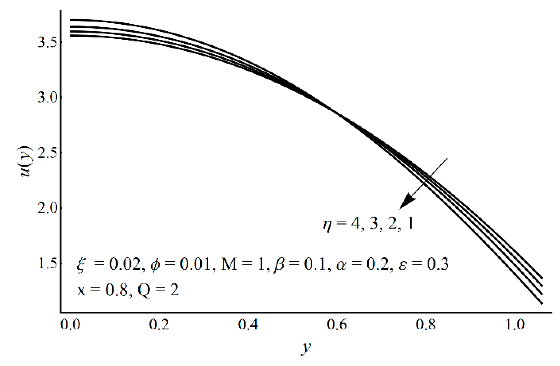
  • The Prandtl fluid material parameter η has increasing effects on the velocity and entropy production near the boundary;
  • Due to wall slip, the velocity increases, while temperature and the entropy production decrease;
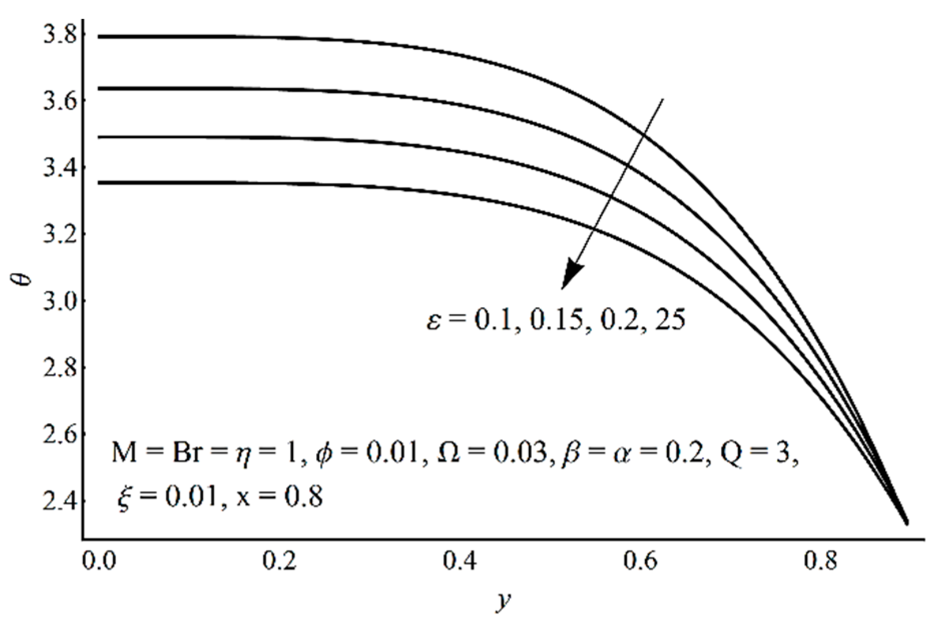
  • The temperature jump brought an increasing change in the temperature profile;
  • Near the channel center, fluid friction irreversibility is dominant, whereas near the heated ciliated wall, the effect of heat transfer irreversibility is noticeable;
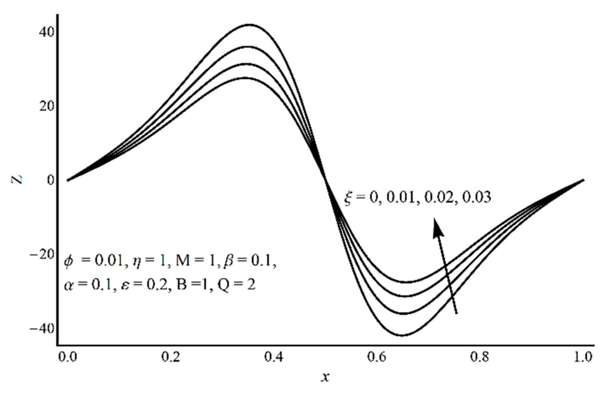
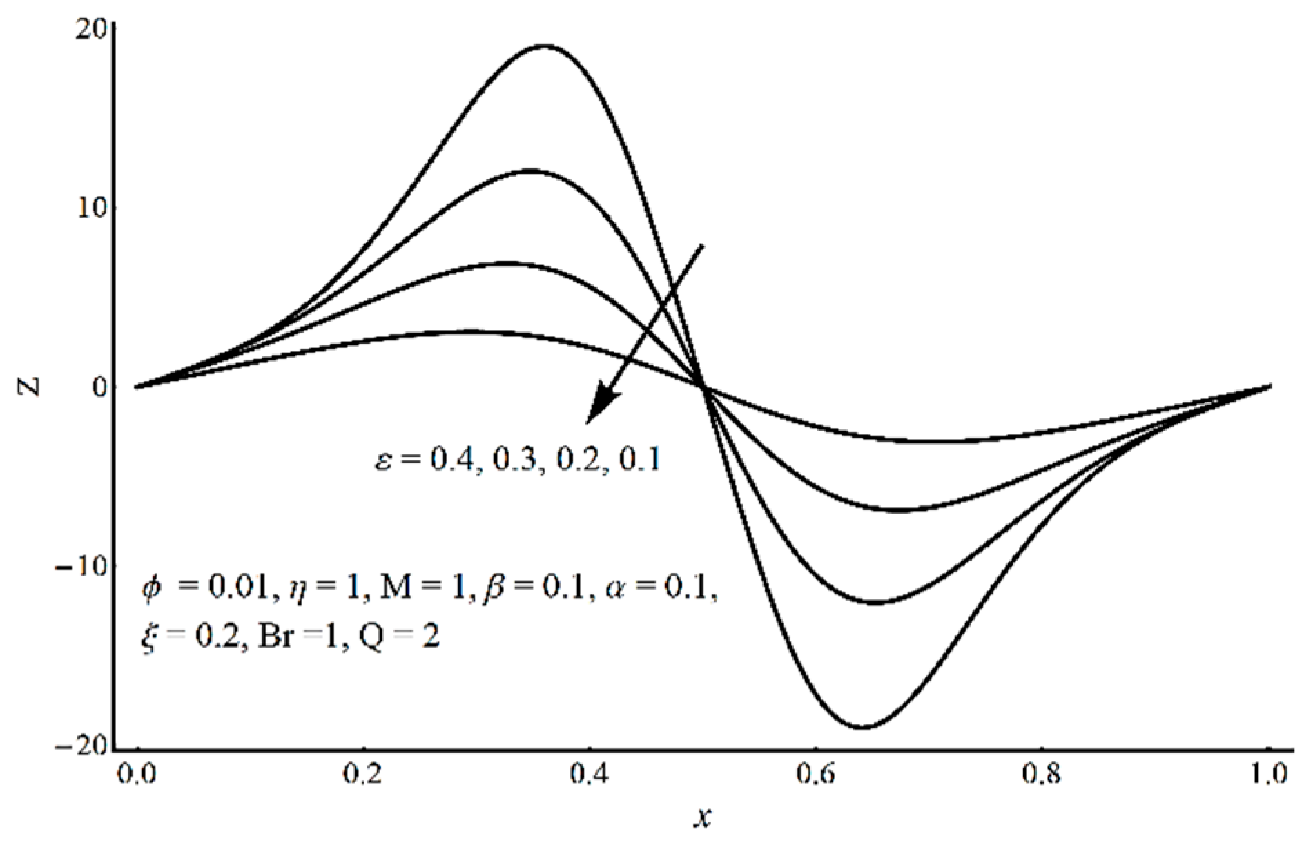
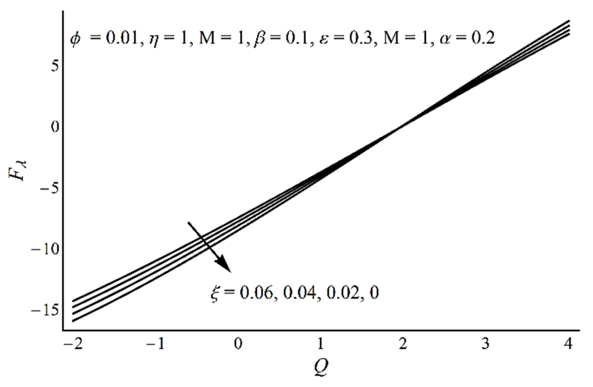
  • In the contracted part, a significant elevation in pressure gradient is achieved for small values of ξ and high values of ε and η;
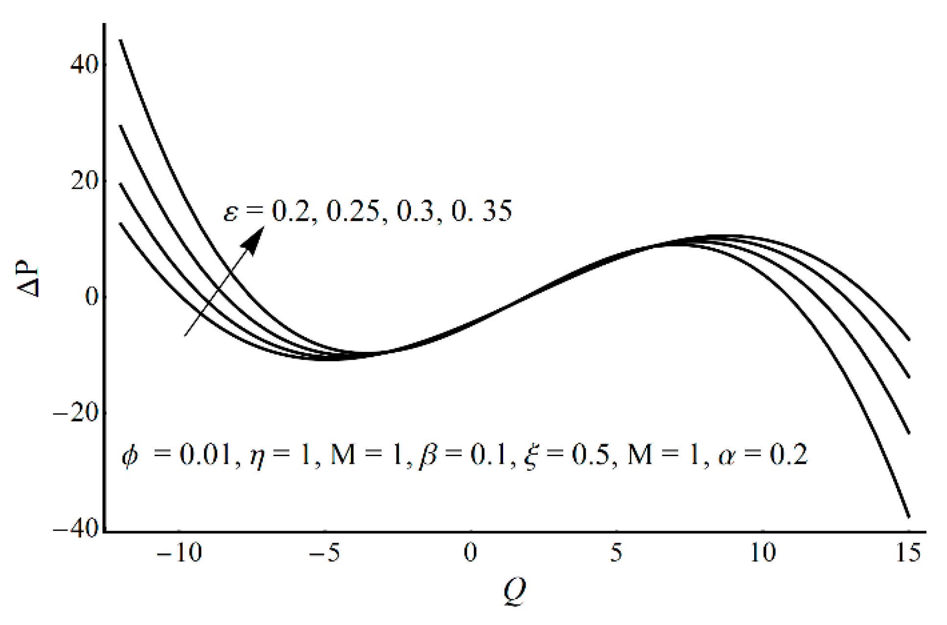
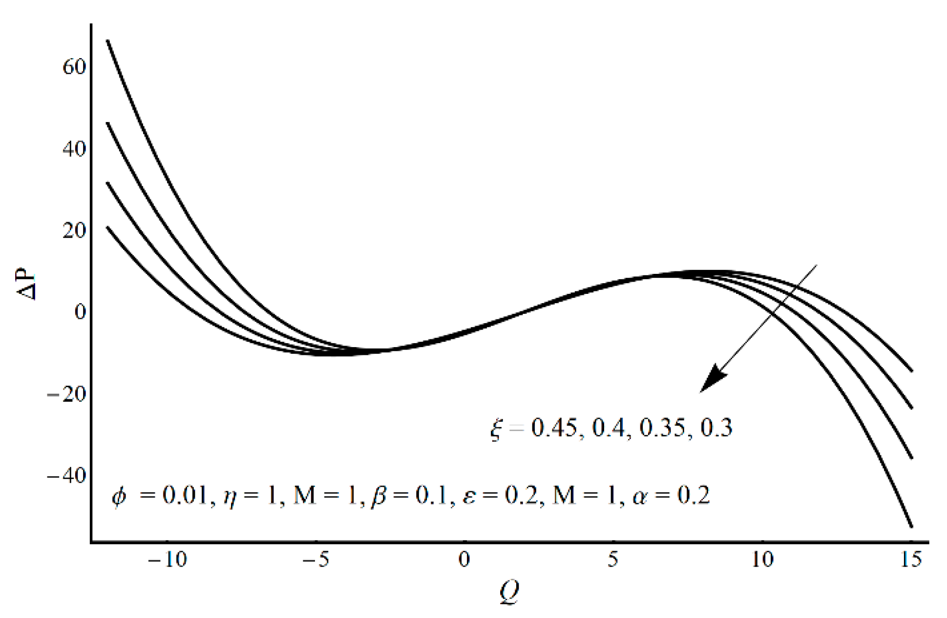
  • Pressure-rise per wavelength increases as ε increases and shows a decreasing trend as ξ and η increase in the pumping part and completely reverse conduct in the augmented pumping part;
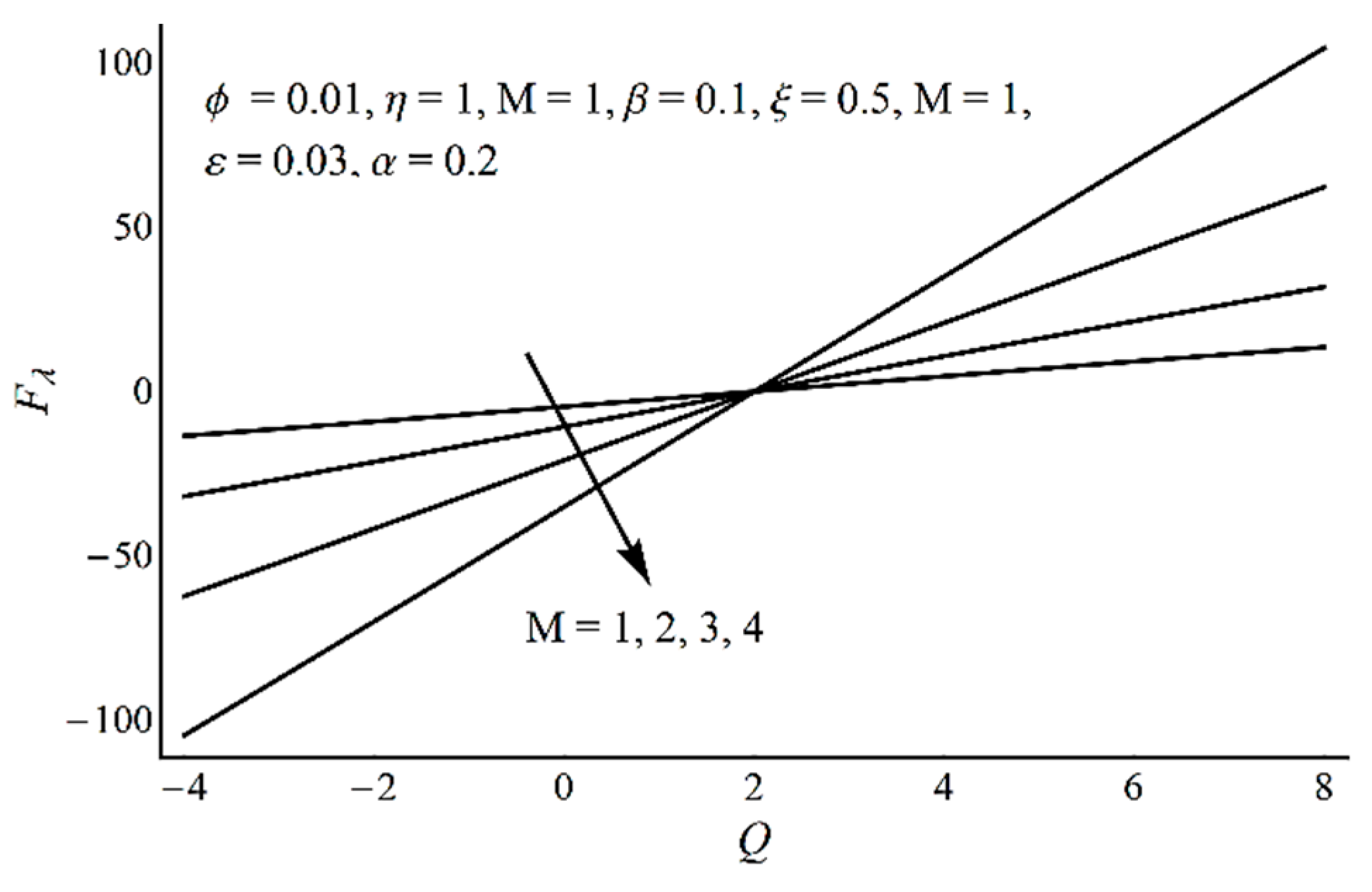
  • Frictional force at the wavy wall explains a direct proportionality with mean flow rate.

Author Contributions

Conceptualization, N.S. and S.M.; methodology, N.S.; software, N.S.; validation, S.M.; formal analysis, S.M.; investigation, N.S. and S.M.; resources, N.S.; data curation, S.M.; writing—original draft preparation, N.S.; writing—review and editing, S.M.; visualization, S.M. and N.S.; supervision, N.S.; project administration, S.M.; funding acquisition, N.S. All authors have read and agreed to the published version of the manuscript.

Funding

This research receives no external funding.

Conflicts of Interest

The authors declare no conflict of interest.

References

  1. Bustamante-Marin, X.M.; Ostrowski, L.E. Cilia and mucociliary clearance. Cold Spring Harb Perspect Biol. 2017, 4, a028241. [Google Scholar] [CrossRef]
  2. Knowles, M.R.; Boucher, R.C. Mucus clearance as a primary innate defense mechanism for mammalian airways. J. Clin. Investig. 2002, 109, 571–577. [Google Scholar] [CrossRef]
  3. Pablo, J.L.; DeCaen, P.G.; Clapham, D.E. Progress in ciliary ion channel physiology. J. Gen. Physiol. 2016, 1, 37–41. [Google Scholar] [CrossRef] [Green Version]
  4. Ghazal, S.; Makarov, J.K.; de Jonge, C.J. Egg transport and fertilization. Glob. Libr. Women Med. 2014, 2014. [Google Scholar] [CrossRef]
  5. Eddy, C.A.; Pauerstein, C.J. Anatomy and physiology of the fallopian tube. Clin. Obstet. Gynecol. 1980, 4, 1177–1193. [Google Scholar] [CrossRef]
  6. Lehti, M.S.; Sironen, A. Formation and function of sperm tail structures in association with sperm motility defects. Biol. Reprod. 2017, 97, 522–536. [Google Scholar] [CrossRef]
  7. Mills, Z.; Aziz, B.; Alexeev, A. Beating synthetic cilia enhance heat transport in microfluidic channels. Soft Matter 2012, 45, 11508–11513. [Google Scholar] [CrossRef]
  8. Drummond, I.A. Cilia functions in development. Curr. Opin. Cell Biol. 2012, 1, 24–30. [Google Scholar] [CrossRef] [Green Version]
  9. Agrawal, H.L. Anawaruddin. Cilia transport of bio-fluid wih variable viscosity. Indian J. Pure Appl. Math. 1984, 15, 1128–1139. [Google Scholar]
  10. Qiu, T.; Lee, T.; Mark, A.G.; Morozov, K.I.; Münster, R.; Mierka, O.; Turek, S.; Leshansky, A.M.; Fischer, P. Swimming by reciprocal motion at low Reynolds number. Nat. Commun. 2014, 5, 1–8. [Google Scholar] [CrossRef] [Green Version]
  11. Brennen, C. Oscillating-boundary layer theory for ciliary propulsion. J. Fluid Mech. 1974, 65, 799–824. [Google Scholar] [CrossRef] [Green Version]
  12. Wu, A.; Abbas, S.Z.; Asghar, Z.; Sun, H.; Waqas, M.; Khan, W.A. A shear-rate-dependent flow generated via magnetically controlled metachronal motion of artificial cilia. Biomech. Model. Mechanobiol. 2020. [Google Scholar] [CrossRef]
  13. Farooq, A.A.; Siddiqui, A.M. Mathematical model for the ciliary-induced transport of seminal liquids through the ductuli efferentes. Int. J. Biomath. 2017, 10, 1750031. [Google Scholar] [CrossRef]
  14. Farooq, A.A.; Tripathi, D.; Elnaqeeb, T. On the propulsion of micropolar fluid inside a channel due to ciliary induced metachronal wave. Appl. Math. Comput. 2019, 347, 225–235. [Google Scholar] [CrossRef]
  15. Stud, V.K.; Sephon, G.S.; Mishra, R.K. Pumping action on blood flow by a magnetic field. Bull. Math. Biol. 1977, 39, 385–390. [Google Scholar]
  16. Mekheimer, K.S. Peristaltic transport of a couple stress fluid in a uniform and non-uniform channels. Biorheology 2002, 39, 755–765. [Google Scholar]
  17. Hatzikonstantinou, P.M.; Vafeas, P. A general theoretical model for the magnetohydrodynamic flow of micropolar magnetic fluids. Application to Stokes flow. Math. Methods Appl. Sci. 2010, 33, 233–248. [Google Scholar] [CrossRef]
  18. Tripathi, D.; Jhorar, R.; Beg, O.A. A KadirElectro-magneto-hydrodynamic peristaltic pumping of couple stress biofluids through a complex wavy micro-channel. J. Mol. Liq. 2017, 236, 358–367. [Google Scholar] [CrossRef]
  19. Akram, S.; Afzal, F.; Imran, M. Influence of metachronal wave on hyperbolic tangent fluid model with inclined magnetic field. Int. J. Geom. Methods. Mod. Phys. 2019, 16, 1950139. [Google Scholar] [CrossRef]
  20. Mekheimer, K.S.; Mohamed, M.S. Interaction of pulsatile flow on the peristaltic motion of a magneto-micropolar fluid through porous medium in a flexible channel: Blood flow model. Int. J. Pure Appl. Math. 2014, 94, 323–339. [Google Scholar] [CrossRef]
  21. Saleem, N.; Hayat, T.; Alsaedi, A. A hydromagnetic mathematical model for blood flow of Carreau fluid. Int. J. Biomath. 2014, 7, 1–14. [Google Scholar] [CrossRef]
  22. Papadopoulos, P.K.; Vafeas, P.; Hatzikonstantinou, P.M. Ferrofluid pipe flow under the influence of the magnetic field of a cylindrical coil. Phys. Fluids 2012, 24, 1–13. [Google Scholar] [CrossRef]
  23. Taherali, F.; Varum, F.; Basit, A.W. A slippery slope: On the origin, role and physiology of mucus. Adv. Drug Deliv. Rev. 2018, 124, 16–33. [Google Scholar] [CrossRef]
  24. Tripathi, D.; Beg, O.A.; Curiel-Sosa, J.L. Homotopy semi-numerical simulation of peristaltic flow of generalised Oldroyd-B fluids with slip effects. Comput. Method. Biomec. 2014, 17, 433–442. [Google Scholar] [CrossRef]
  25. Makinde, O.D.; Reddy, M.G.; Reddy, K.V. Effects of thermal radiation on MHD peristaltic motion of walters-B fluid with heat source and slip conditions. J. Appl. Fluid Mech. 2017, 10, 1105–1112. [Google Scholar] [CrossRef]
  26. Akram, S. Effects of slip and heat transfer on a peristaltic flow of a Carreau fluid in a vertical asymmetric channel. Comp. Math. Math. Phys. 2014, 54, 1886–1902. [Google Scholar] [CrossRef]
  27. Akbar, N.; Nadeem, S. Thermal and velocity slip effects on the peristaltic flow of a six constant Jeffrey’s fluid model. Int. J. Heat Mass Tran. 2012, 55, 3964–3970. [Google Scholar] [CrossRef]
  28. Makinde, O.D. Entropy analysis for MHD boundary layer flow and heat transfer over a flat plate with a convective surface boundary condition. Int. J. Exergy 2012, 10, 142–154. [Google Scholar] [CrossRef]
  29. Adesanya, S.O.; Makinde, O.D. Thermodynamic analysis for a third-grade fluid through a vertical channel with internal heat generation. J. Hydrodyn. 2015, 27, 264–272. [Google Scholar] [CrossRef]
  30. Chamkha, A.J.; Selimefendigil, F. MHD free convection and entropy generation in a corrugated cavity filled with a porous medium saturated with nanofluids. Entropy 2018, 20, 846. [Google Scholar] [CrossRef] [Green Version]
  31. Butt, A.S.; Ali, A.; Munawar, S. Slip effects on entropy generation in MHD flow over a stretching surface in the presence of thermal radiation. Int. J. Exergy. 2013, 13, 1–20. [Google Scholar] [CrossRef]
  32. Bejan, A. A study of entropy generation in fundamental convective heat transfer. J. Heat Transf. 1979, 101, 718–725. [Google Scholar] [CrossRef]
  33. Bejan, A. Second-law analysis in heat transfer and thermal design. Adv. Heat Transf. 1982, 15, 1–58. [Google Scholar]
  34. Souidi, F.; Ayachi, K.; Benyahia, N. Entropy generation rate for a peristaltic pump. J. Non-Equilib. Thermodyn. 2009, 34, 171–194. [Google Scholar] [CrossRef]
  35. Akbar, N.S. Entropy generation and energy conversion rate for the peristaltic flow in a tube with magnetic field. Energy 2015, 82, 23–30. [Google Scholar] [CrossRef]
  36. Saleem, N. Entropy production in peristaltic flow of a space dependent viscosity fluid in asymmetric channel. Therm. Sci. 2018, 22, 2909–2918. [Google Scholar] [CrossRef]
  37. Munawar, S.; Saleem, N.; Aboura, K. Second law analysis in the peristaltic flow of variable viscosity fluid. Int. J. Exergy 2016, 20, 170–185. [Google Scholar]
  38. Saleem, N.; Munawar, S. Entropy analysis in cilia driven pumping flow of hyperbolic tangent fluid with magnetic field effects. Fluid Dyn. Res. 2020, 52, 2. [Google Scholar] [CrossRef]
  39. Siddiqui, A.M.; Farooq, A.A.; Rana, M.A. Hydromagnetic flow of Newtonian fluid due to ciliary motion in a channel. Magnetohydrodynamics 2014, 50, 109–122. [Google Scholar]
  40. Ramesh, K.; Tripathi, D.; Beg, O.A. Cilia-assisted hydromagnetic pumping of biorheological couple stress fluids. J. Propul. Power 2019, 8, 221–233. [Google Scholar] [CrossRef]
  41. Alsaedi, A.; Batool, N.; Yasmin, H.; Hayat, T. Convective heat transfer analysis on prandtl fluid model with peristalsis. Appl. Bionic. Biomech. 2013, 10, 197–208. [Google Scholar] [CrossRef]
  42. Patel, M.; Timol, M.G. The stress strain relationship for viscous-inelastic non-Newtonian fluids. Int. J. Appl. Math. Mech. 2010, 6, 79–93. [Google Scholar]
  43. Hayat, T.; Saleem, N.; Ali, N. Peristaltic flow of a Carreau fluid in a channel with different wave forms. Numer. Meth. Part. Differ. Equ. 2010, 26, 519–534. [Google Scholar] [CrossRef]
  44. Tripathi, D. A mathematical model for the peristaltic flow of chyme movement in small intestine. Math. Biosci. 2011, 233, 90–97. [Google Scholar] [CrossRef]
  45. Mehmood, O.U.; Mustapha, N.; Shafie, S. Heat transfer on peristaltic flow of fourth grade fluid in inclined asymmetric channel with partial slip. Appl. Math. Mech. 2012, 33, 1313–1328. [Google Scholar] [CrossRef] [Green Version]
  46. Jothi, S.; Prasad, A.R.; Reddy, M.V.S. Peristaltic flow of a Prandtl fluid in a symmetric channel under the effect of a magnetic field. Adv. Appl. Sci. Res. 2012, 3, 2108–2119. [Google Scholar]
  47. Bejan, A. Second law analysis in heat transfer. Energy 1980, 5, 720–732. [Google Scholar] [CrossRef]
  48. Munawar, S.; Saleem, N. Second law analysis of ciliary pumping transport in an inclined channel coated with carreau fluid under a magnetic field. Coatings 2020, 10, 240. [Google Scholar] [CrossRef] [Green Version]
Figure 1. Physical geometry of the fluid flow in ciliated channel.
Coatings 10 00414 g001
Figure 2. Comparison of the velocity profile of the present work with the velocity profile reported by Jothi [46].
Coatings 10 00414 g002
Figure 3. Axial velocity for various values of velocity slip parameter ξ.
Coatings 10 00414 g003
Figure 4. Axial velocity for various values of cilia length parameter ε.
Coatings 10 00414 g004
Figure 5. Axial velocity for different values of time relaxation parameter ϕ.
Coatings 10 00414 g005
Figure 6. Axial velocity for various values of fluid material parameter η.
Coatings 10 00414 g006
Figure 7. Pressure gradient at various values of variable ε.
Coatings 10 00414 g007
Figure 8. Pressure gradient at various values of variable ξ.
Coatings 10 00414 g008
Figure 9. Pressure gradient at various values of variable η.
Coatings 10 00414 g009
Figure 10. Pressure-rise per wavelength at various values of ε.
Coatings 10 00414 g010
Figure 11. Pressure-rise per wavelength at various values of ξ.
Coatings 10 00414 g011
Figure 12. Pressure-rise per wavelength at various values of η.
Coatings 10 00414 g012
Figure 13. The temperature profile against various values of velocity slip parameter ξ.
Coatings 10 00414 g013
Figure 14. The temperature profile against various values of temperature jump Ω.
Coatings 10 00414 g014
Figure 15. The temperature profile against various values of cilia length parameter ε.
Coatings 10 00414 g015
Figure 16. The temperature profile against various values of the Hartmann number M.
Coatings 10 00414 g016
Figure 17. The total entropy generation number against various ε values.
Coatings 10 00414 g017
Figure 18. The Bejan number against various ε values.
Coatings 10 00414 g018
Figure 19. The total entropy generation number against various material parameter η values.
Coatings 10 00414 g019
Figure 20. The total entropy generation number against various α values.
Coatings 10 00414 g020
Figure 21. The total entropy generation number against various ξ values.
Coatings 10 00414 g021
Figure 22. The Bejan number against various ξ values.
Coatings 10 00414 g022
Figure 23. The total entropy generation number against variables x and y, when M = Br = 1, ε = 0.2, α = 0.1, ϕ = 0.01, β = 0.5, ξ = 0.05, η = 1.
Coatings 10 00414 g023
Figure 24. The Bejan number against variables x and y, when M = Br = 1, ε = 0.2, α = 0.1, ϕ = 0.01, β = 0.5, ξ = 0.05, η = 1.
Coatings 10 00414 g024
Figure 25. Heat transfer coefficient at the ciliated channel wall for different values of ξ.
Coatings 10 00414 g025
Figure 26. Heat transfer coefficient at the ciliated channel wall for different values of ε.
Coatings 10 00414 g026
Figure 27. Variations of frictional forces for different values of M.
Coatings 10 00414 g027
Figure 28. Variations in frictional forces for different values of ε.
Coatings 10 00414 g028
Figure 29. Variations in fluid frictional forces at various ξ.
Coatings 10 00414 g029
Figure 30. Streamlines at two different values of ε, when α = 0.2, ϕ = 0.01, β = 0.5, ξ = 0.02, η = M = 1, Q = 0.4: (a) ε = 0.4; (b) ε = 0.45.
Coatings 10 00414 g030
Figure 31. Streamlines at two different values of ξ when α = 0.2, ϕ = 0.01, ε = β = 0.5, M = η= 1, Q = 0.4: (a) ε = 0; (b) ε = 0.06.
Coatings 10 00414 g031
Figure 32. Streamlines for two different values of M, when α = 0.2, ϕ = 0.01, ε = β = 0.5, ξ = 0.02, η = 1, Q = 0.4: (a) M = 0.5; (b) M = 1.
Coatings 10 00414 g032

