Simulation of Magnetic-Field-Induced Ion Motion in Vacuum Arc Deposition for Inner Surfaces of Tubular Workpiece

Abstract

A simulation of magnetic-field-induced ion motion in vacuum arc deposition for the inner surfaces of a tubular workpiece was performed. An auxiliary magnetic field was set to guide the motion of ions inside a pipe, with different magnetic flux densities and ion emission parameters. The results showed the trajectories, deposition ratio and depth of the ions can be controlled via a magnetic field. Within a certain range, the deposition ratio of the ions increases with magnetic flux density. When the magnetic flux density reached a certain value, both the trajectories and deposition ratio of the ions exhibited an obvious periodicity. The depth at which the ions were deposited decreased as an exponential function of the magnetic flux density and ion emission radius, respectively. With an increase in the emission angle, the deposition depth decreased linearly. A numerical model was proposed to express the distribution of the deposition depth. In addition, the deposition ratio and depth are improved with a magnetic field in an environment with a certain density of neutral gas.

1. Introduction

In many areas of industrial application, the inner surfaces of tubular workpieces are usually prone to early failure due to wear, corrosion and oxidation [1,2], resulting in considerable economic losses. The improvement of inner surface quality is often required. Research shows that surface-coating technology is an effective means to solve this problem [3,4,5,6,7,8].

Vacuum arc deposition (VAD) is one of the important coating technologies characterized by a high ionization rate (60%~90%) with a high plasma density 10¹⁷~10¹⁸ m⁻³ [9]. VAD is often used to prepare wear-resistant hard coatings such as metallic nitrides. Because of the geometrical shadowing effect of tubular workpieces, it is difficult for ions to deposit on the deep inside surface of the tube. According to Shi et al. [10], the thickness, hardness and wear resistance of the deposited coating obviously decreases as the distance from the pipe inlet increases. Hence, there are still some problems to be solved when VAD is used for inner surface coating.

Studies have shown that a magnetic field can be used to guide the motion of ions [11,12,13,14,15,16,17]. Magnetic fields were commonly used to control the motion of cathode spots [12,13,14], and were also introduced to guide ion motion and to remove the macro-particles from the arc source [15,16,17]. Therefore, controlling the movement of deposition ions may be beneficial for the deposition of inner surface coating.

Aksenov et al. [18] set a solenoid near or around a metallic pipe and found that the deposition rate for the VAD coating inside the pipe was improved by the magnetic field. Later on, a magnetic field was used to increase the coating deposition depth and thickness inside tubular workpieces [19]. Liu et al. [20] set a permanent magnet alongside a 50 mm inner diameter pipe for depositing TiN coating, and the ratio of the deposition depth to the pipe diameter increased from 1:1 to 2:1 compared to that without a magnetic field. Because of the demagnetization during deposition, the application of permanent magnets has been limited [21]. Lang et al. [22] developed an axially decreased magnetic field around a pipe with an inner diameter of 20 mm for the deposition of (Ti,Al)N coatings. The results showed that the deposition depth-pipe diameter ratio was 6:1, and the deepest coating thickness inside the pipe was 20% of that at the pipe inlet. Zhao et al. [23] used a strengthened magnetic field for a pipe with an inner diameter of 36 mm; a coating depth-pipe diameter ratio of 4:1 was achieved, and the deepest coating thickness inside the pipe reached 60% that of the pipe inlet. Lisenkov et al. [24] used the magnetic field generated by a single coil coaxial placed between the ion source and 10~50 mm inner diameter pipes, and deposited TiC coating inside the pipe. The ratio of the coating deposition depth to the pipe diameter reached 8:1, while the deepest coating thickness inside the pipe was about 40% of that at the pipe inlet.

To further improve the proportion of ions deposited inside tubular workpieces under a magnetic field, it is necessary to study the ion motion under different magnetic fields. Simulation provides an effective way to study the effect of a magnetic field on ion motion. Because the mean free path of ions significantly increases under a certain vacuum, Birdsall et al. [25] put forward the idea of particle simulation. Skullerud et al. [26] developed a tracing simulation scheme to calculate the trajectory of charged particles under an external electric field including the Monte-Carlo collision scheme, which provides a method to investigate the ion motion with an external field. Li et al. [27] used the tracing method to calculate the ion motion of carbon ions within the symmetric plane of a bended magnetic filter, and the ion motion could be controlled via the magnetic field to increase the filter efficiency. Takahashi et al. [28] used the tracing method to study the effect of a magnetic field on the ion motion of a laser ion source. The results showed that the magnetic field could affect the ion motion to increase the output ion current.

In this paper, the simulation of magnetic field-induced ion motion in vacuum arc deposition for the inner surfaces of a tubular workpiece was studied. The effect of a magnetic field on ion motion was studied using 3D ion tracing simulation coupled with magnetic field simulation. The influence of ion-neutral elastic collision is also discussed.

2. Materials and Methods

2.1. Simulation Setup

Figure 1 shows the schematic diagram of the vacuum arc deposition system (State Key Laboratory of Tribology, Beijing, China) for the inner surface of a pipe. The pipe and the coil were coaxial with the ion source. The symmetric plane of the coil was aligned with the pipe. The current of the coil was adjustable and was kept ideally static. If an ion reached any surface of the solid part in the simulation region, its location was considered unchanged. Secondary emission was neglected because of its low energy [29]. It was possible to evaluate the effect of a magnetic field by calculating the percentage and the depth distribution of ions that were deposited onto the inner surface of the pipe. The actual deposition process was usually performed under a gas environment. Although neutral molecules are not affected by a magnetic field, the collision between ions and background gas molecules would change the ions’ trajectories. Because ionization has relatively less effect on ion trajectories, only the elastic scattering process caused by collision was studied.

The magnetic field distribution generated by the auxiliary coil was simulated according to the Maxwell Equation [30] for the static situation, as shown in Equations (1) and (2).

$$\nabla \times \stackrel{\rightharpoonup }{H}=\stackrel{\rightharpoonup }{J}$$

(1)

$$\nabla \times \stackrel{\rightharpoonup }{A}=\stackrel{\rightharpoonup }{B}$$

(2)

Here, $\stackrel{\rightharpoonup }{H}$ is the magnetic field strength vector, $\stackrel{\rightharpoonup }{B}$ is the magnetic flux density vector, $\stackrel{\rightharpoonup }{J}$ is the total current vector and $\stackrel{\rightharpoonup }{A}$ is the magnetic potential vector. The constitutive relationship of the magnetic field is shown in Equation (3), where $\mathsf{\mu }$ is the relative permeability.

$$\stackrel{\rightharpoonup }{B}=\mathsf{\mu }\stackrel{\rightharpoonup }{H}$$

(3)

Assuming that there were no dielectric matter and charge accumulation, the displacement current could be neglected. Therefore, the conduction current of the auxiliary coil consisted of two items, namely, the induced current ${\stackrel{\rightharpoonup }{J}}_e$ generated by the change in the magnetic field and current ${\stackrel{\rightharpoonup }{J}}_S$ from the power supply (Equation (4)).

$$\stackrel{\rightharpoonup }{J}={\stackrel{\rightharpoonup }{J}}_S+{\stackrel{\rightharpoonup }{J}}_e$$

(4)

Because the ion motion was simulated under a stationary magnetic field, the current ${\stackrel{\rightharpoonup }{J}}_e$ generated by the initial change in the magnetic field could be neglected. Therefore, once the current ${\stackrel{\rightharpoonup }{J}}_S$ was determined, Equation (5) could be obtained as follows according to Equations (1)–(4).

$$\nabla \times \left(\nabla \times \stackrel{\rightharpoonup }{A}\right)={\nabla }^2\stackrel{\rightharpoonup }{A}=\mathsf{\mu }\stackrel{\rightharpoonup }{J}=\mathsf{\mu }{\stackrel{\rightharpoonup }{J}}_S$$

(5)

Equation (5) is a second-order partial differential equation. $\stackrel{\rightharpoonup }{A}$ could be calculated by using the COMSOL© software (version 5.4a). Then, the magnetic strength vector $\stackrel{\rightharpoonup }{B}$ could be solved by using Equation (2); the spatial distribution of the magnetic field could thus be obtained. Furthermore, with the simulation result for the magnetic field, according to the Lorentz force and Newton’s Law, the velocities of the ions could be tracked with the initial position (Equation (6)).

$$m_{ion}\frac{d}{dt}\left({\stackrel{\rightharpoonup }{v}}_{ion}\right)={\stackrel{\rightharpoonup }{F}}_{ion}=Ze{\stackrel{\rightharpoonup }{v}}_{ion}\times \stackrel{\rightharpoonup }{B}$$

(6)

where Z represents the charge number of the ions and e represents the elementary charge. By integrating the velocity of the ions, the positions of the ions could be obtained. Therefore, the 3D trajectories of the ions could be obtained following the iterations according to Equation (6). The simulation result for the magnetic field was set as the input of the Lorentz force. The ion motion was calculated using second-order backward differentiation [31]. In addition, the convergence criterion was set as the error between iterations. The iteration results were discriminated as convergence when the error between iterations was less than or equal to 0.1%. To avoid system crashes due to divergence during the iterations, the stoppage criterion was set to 100 steps for a single iteration. The simulations of both the magnetic field and ion motion were carried out with the same convergence and stoppage criteria.

Research has shown that near the substrate, ions become accelerated when crossing through the sheath [32,33]. However, with the assumption of neglecting plasma instabilities [34,35], the sheath thickness could be determined [36] and would decrease under a magnetic field [37,38]. Therefore, the acceleration mainly influenced the ion velocity, and happened near the workpiece surfaces. Consequently, the impact of the sheath and electric force on ion motion could be neglected. Studies show that under a magnetic field, electrons are confined along magnetic lines, and charge separation occurs to generate electric field dragging [11,17]. According to Aksenov et al. [39], the proportion of ions influenced by the dragging electric field was usually below 10%. Hence, the effect of the dragging electric force on the ions’ trajectories was neglected.

2.2. Setup of Ion-Neutral Collision

The structure and properties of films are affected by temperature and pressure during deposition. The temperature and pressure of the gas were set to 300 °C and 0.1 Pa, respectively. Argon was selected as the background gas, and was considered to be uniformly distributed. According to the ideal gas law, the number density of molecular argon was calculated as 1.26 × 10¹⁹ m⁻³. Compared to the velocity of the ions, the velocity of gas thermal motion (about 15~20 m/s) was slow and neglected. A Monte-Carlo collision scheme [40] was conducted with Equations (7) and (8) based on the conservation of momentum.

$$\mathsf{\nu }=n\mathsf{\sigma }\left|\stackrel{\rightharpoonup }{u}\right|=n\pi {\left(r_i+r_g\right)}^2\left|\stackrel{\rightharpoonup }{u}\right|$$

(7)

$${\stackrel{\rightharpoonup }{u}}^{\prime }=\stackrel{\rightharpoonup }{u}-\frac{m_g}{m_i+m_g}\left(\stackrel{\rightharpoonup }{u}-\left|\stackrel{\rightharpoonup }{u}\right|\stackrel{\rightharpoonup }{k}\right)$$

(8)

In Equation (7), $\mathsf{\nu }$ is the collision frequency determined by the gas molecular number density $n$, ion velocity $\left|\stackrel{\rightharpoonup }{u}\right|$ and collision cross-section $\mathsf{\sigma }$ (6.92 × 10⁻²⁰ m², calculated by the radius of the ion and gas, $r_i$ and $r_g$). The collision probability was estimated as $P=1-\exp \left(-v\Delta t\right)$, where $\Delta t$ is the time step length. In the transient simulation, at the beginning of each time step, a comparison was conducted to judge the happening of collision. For each ion, a random number $U$ uniformly distributed in 0~1 was generated. The collision was considered to occur when $U<P$, and vice versa.

The post-collision velocity ${\stackrel{\rightharpoonup }{u}}^{\prime }$ is described through Equation (8). Because the relative velocity $\stackrel{\rightharpoonup }{u}$ only changes direction after a random elastic collision, a uniformly distributed random unit vector $\stackrel{\rightharpoonup }{k}$ was introduced to describe the direction change. $m_i$ and $m_g$ represent the masses of the ion and gas molecule, respectively.

2.3. Boundary Condition and Meshing Scheme

In order to increase the computation efficiency in the simulation of the magnetic field, the magnetic field was constrained within the boundary of the simulation region. The Dirichlet boundary condition [30] was applied, where the tangential components of the magnetic potential were set to zero (Equation (9)).

$$\widehat{n}\times \stackrel{\rightharpoonup }{A}=0$$

(9)

Here, $\widehat{n}$ represents the normal vector of the boundary surface and $\stackrel{\rightharpoonup }{A}$ represents the magnetic potential vector. The simulated magnetic field near the boundary of the simulation region would be different from the actual distribution. In order to reduce the influence of the boundary difference on the simulation results, the meshing scheme as shown in Figure 2a was conducted. Considering the symmetry, the simulation region was set as a sphere with a radius of 2 m. Outside the sphere, a shell with a thickness of 0.5 m was set by means of the infinite-element method [41,42], which uses a coordinate transformation to scale the shell to 1000 times larger. The Dirichlet boundary condition was set at the outmost surface of the shell. To ensure the continuation of the simulation region and the boundary shell, the shape function was defined as Lagrange polynomials using the coordinate inside the simulation region and the shell, and the interpolation function for the magnetic field simulation was set the same as the shape function. With the setting of the large-scaled shell, the difference in the magnetic field near the boundary could be controlled within the shell, and would not affect the result inside the simulation region.

Tetrahedral volume elements were used to construct the mesh. Figure 2b shows the meshing scheme of the arc source, the pipe and the coil. To avoid the disturbance of sharp geometric corners, the size of the elements would change with a side length changing factor of 0~0.1 to connect different mesh regions. In addition, the size of the minimum mesh element was set as 0.5 mm.

Table 1. Geometric parameters of the simulation.

Coil Cross-Section (mm × mm)	Wire Cross-Section Area (mm2)	Coil Inner Diameter (mm)	Coil Outer Diameter (mm)
60 × 60	1	135	255
Source Diameter (mm)	Pipe Inner Diameter (mm)	Pipe Length (mm)	Pipe Wall Thickness (mm)
100	50	200	4

shows the geometric information for meshing. The distance between the pipe entrance and arc source was 400 mm.

2.4. Simulation Parameters of Ion Emission

Table 2. Emission parameters of Ti ion.

Ion Mass (kg)	Ion Charge State	Initial Kinetic Energy (eV)	Simulation Timespan (s)
7.95 × 10−26	+2 [43]	100 [44,45]	1 × 10−4

shows the attributes of the Ti ion used for this simulation. The charge state +2 was used according to the average charge state measured by Jüttner et al. [43]. The initial kinetic energy was set as 100 eV. Therefore, the initial ion velocity was 2 × 10⁴ m/s, which was in accordance with the average of the velocity range 1~3 × 10⁴ m/s for Ti ions measured by Kutzner and Byon et al. [44,45]. Considering the velocity of the Ti ion, the step length of the simulation was set as 5 × 10⁻⁸ s. The spatial location change of the Ti ion was within 1 mm per time step. Because the ion Larmor radius (e.g., calculated as 10 mm using the magnetic flux density 5000 Gs) is larger than 1 mm, the step length was reasonable for describing the ion trajectories.

Figure 3 shows the 2D axial-symmetric view of the ion’s initial velocity direction. α is the angle between the emission direction of the ion and the X-axis. Research shows that the ion flux of a vacuum arc discharge follows the cosine law or cosine square law [46,47,48], which means that the ion density is relatively high close to the cathode center axis. With the existence of an axillary magnet in the arc source, the ion emission angle decreases by 50% compared to the pattern of the cosine law [49], making the ion flux more centered. Hence, in the simulation, the range of α was set within 10°. In consideration of the symmetry and simplification, the velocity of the ions was set away from the center axis, representing the emission of ions.

3. Results

3.1. Magnetic Field Distribution

Figure 4 shows the magnetic flux density distribution with the coil current of 7.5 A. An X–R cross-section image of the magnetic flux density distribution is shown in Figure 4a with a color bar. Small arrows represent the direction of the magnetic vector. The field was relatively strong near the coil, and symmetric around the X-axis. The magnetic flux density along the X-axis is shown in Figure 4b. The magnetic flux intensity along the R-direction in the center plane (X = 400 mm) is shown in Figure 4c. The magnetic field along the X-axis had a Gaussian distribution with a maximum value of 1725 Gs. The field distribution along the coil diameter was parabolic with a minimum value in the center. Since the field distribution inside the coil winding was difficult to solve due to the existence of charge [50], Figure 4c only shows the field distribution within the range of the coil inner diameter.

The magnetic flux density at the coil center was recognized to represent the magnetic field of the coil [50]. Herein, the magnetic flux density at the coil center was defined as the characteristic magnetic flux density. It is shown in Figure 5 that the simulated characteristic magnetic flux density was proportional to the coil current. In the following simulation, the coil current ranging from approximately 0 to 20 A with an interval of 0.25 A was adopted, corresponding to the range 0~4600 Gs for the characteristic magnetic flux density with an interval of 57 Gs.

3.2. Magnetic-Field-Induced Motion of Ions

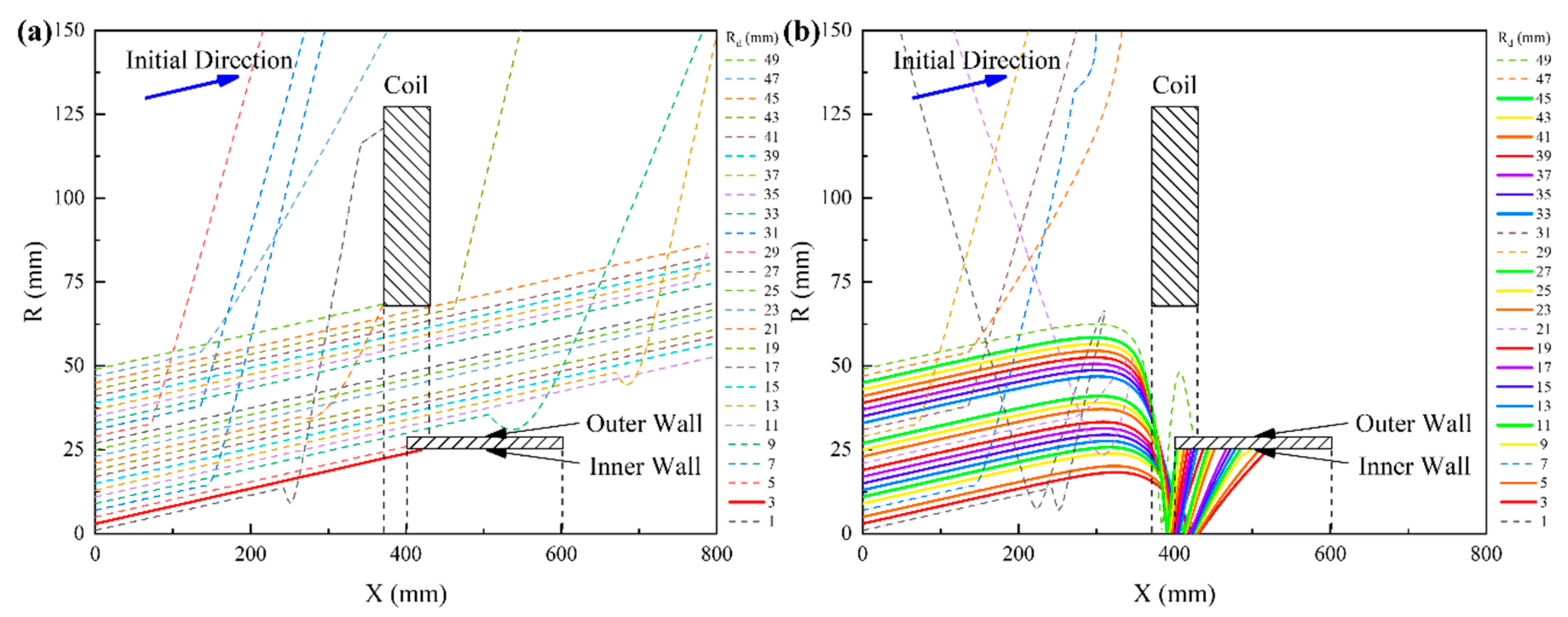
3.2.1. Effect of Magnetic Field on the Motion of Horizontally Emitted Ions

The motion of horizontally emitted ions without a magnetic field was simulated. To describe the initial positions of the ions, the emission radius (R) was defined as the distance between the ions’ initial positions and the center of the target surface. Figure 6 shows the trajectories (dashed lines) of the horizontally emitted ions with different emission radii. Without a magnetic field, the ions could not be deposited on the inner surface of the pipe.

Figure 7 shows the trajectories of the horizontally emitted ions under different characteristic magnetic flux densities. The solid lines represent the trajectories of the deposited ions, and the dashed lines represent other ions. Figure 7a–c show that the ions were blocked by the pipe or moved through the pipe when the characteristic magnetic flux density was less than 920 Gs. When the characteristic magnetic flux density was 977 Gs, the deposition of the ions occurred at the outlet of the pipe (Figure 7d). With an increase in the characteristic magnetic flux density, the number of deposited ions increased (Figure 7e). However, as the characteristic magnetic flux density further increased, the number of deposited ions decreased, and ions started to return to the center axis (Figure 7f). As the characteristic magnetic flux density kept increasing, the number of deposited ions increased again (Figure 7g,h). The phenomenon of the increase and decrease in the number of deposited ions presented a periodicity as the characteristic magnetic flux density increased.

The ions focusing close to the center axis near the pipe inlet caused by the magnetic-field-guided motion can be regarded as the magnetic mirror effect [51]. With the increase in the characteristic magnetic flux density, the ions were driven to make spiral motions along the magnetic induction line, which caused a return towards the center axis before deposition. Therefore, it took a longer period of time for the ions inside the pipe. The maximum number of deposited ions would decrease for higher field intensities. In addition, the reason for some ions moving through the pipe was that the direction of the magnetic field turned to be parallel to the center axis close to the coil center, making the Lorentz force too small for the horizontally emitted ions with small emission radii to deposit.

Figure 8 shows the deposition distance from the pipe inlet of the ions, which is defined as the deposition depth in Figure 1. The deposition depth decreased with the emission radius. When the characteristic magnetic flux density was less than 977 Gs, the ions could not deposit on the inner surface because of the insufficient direction change. As the characteristic magnetic flux density increased to 1840 Gs, the inner surface of the pipe was gradually covered by ions from the outlet towards the inlet of the pipe. As the characteristic magnetic flux density further increased to 2622 Gs, some of the ions started to deposit back to the outlet due to the return motion. Furthermore, with the increase in the characteristic magnetic flux density to 3450 Gs, the ions deposited continually from the outlet towards the inlet of the pipe after a spiral, showing a trend of periodicity. For the characteristic magnetic flux density of 4600 Gs, the deposition depth firstly decreased and then increased when R > 45 mm, because of a new returning motion making some ions deposit inside the pipe. An exponential fitting for the simulation results for the deposition depth was made and is shown in Figure 8. Based on the exponential fitting, a deposition depth model is proposed below.

$$D=D_B{e}^{-B/B_0}+D_R{e}^{-R/R_0}$$

(10)

In this model, the deposition depth D (unit: mm) is determined by two terms. The first exponential item describes the effect of the characteristic magnetic flux density B (unit: Gs) on the deposition depth of the ions; the second exponential item reflects the effect of the ion’s initial distance R (unit: mm) away from the source center. Here, D_B, B₀, D_R and R₀ are constants determined by the attributes of the ion and the geometric parameter of the pipe. The values D_B = 3290.6 mm, B₀ = 305.3 Gs, D_R = 387.6 mm and R₀ =17.3 mm were obtained by fitting the simulation results. Therefore, given the initial location of the ion and characteristic magnetic flux density, the deposition depth could be predicted. The decreasing exponential model is similar to the exponential ion current shrinking pattern in the filter pipe obtained by Boerker et al. [52], Cluggish [53], Kelly et al. [54] and Zhitomirsky et al. [55]. Furthermore, the model may be used to explain the film thickness curve obtained in some experimental results shown in the literature [20,22,23,24].

To evaluate the effectiveness of the model,

Table 3. Adjusted coefficient of the deposition depth model.

Characteristic Magnetic Flux Density (Gs)	Adjusted Coefficient	Characteristic Magnetic Flux Density (Gs)	Adjusted Coefficient
1035	0.998	2530	0.571
1150	0.954	2622	0.121
1380	0.791	2760	0.125
1610	0.976	2990	0.591
1840	0.991	3450	0.708
2070	0.976	4600	0.008
2300	0.714	-	-

shows the adjusted coefficient of determination [56] of the model under different characteristic magnetic flux densities. The adjusted coefficient is a normalized number defined according to the error between the fitting and original simulated results.

The closer the coefficient is to 1, the more reliable the fitting is. In most cases, the adjusted coefficients of the model were above 0.7. As for the cases with low adjusted coefficients, the number of ions with returning motion varied for different emission radii, which made it difficult for exponential fitting to describe the results.

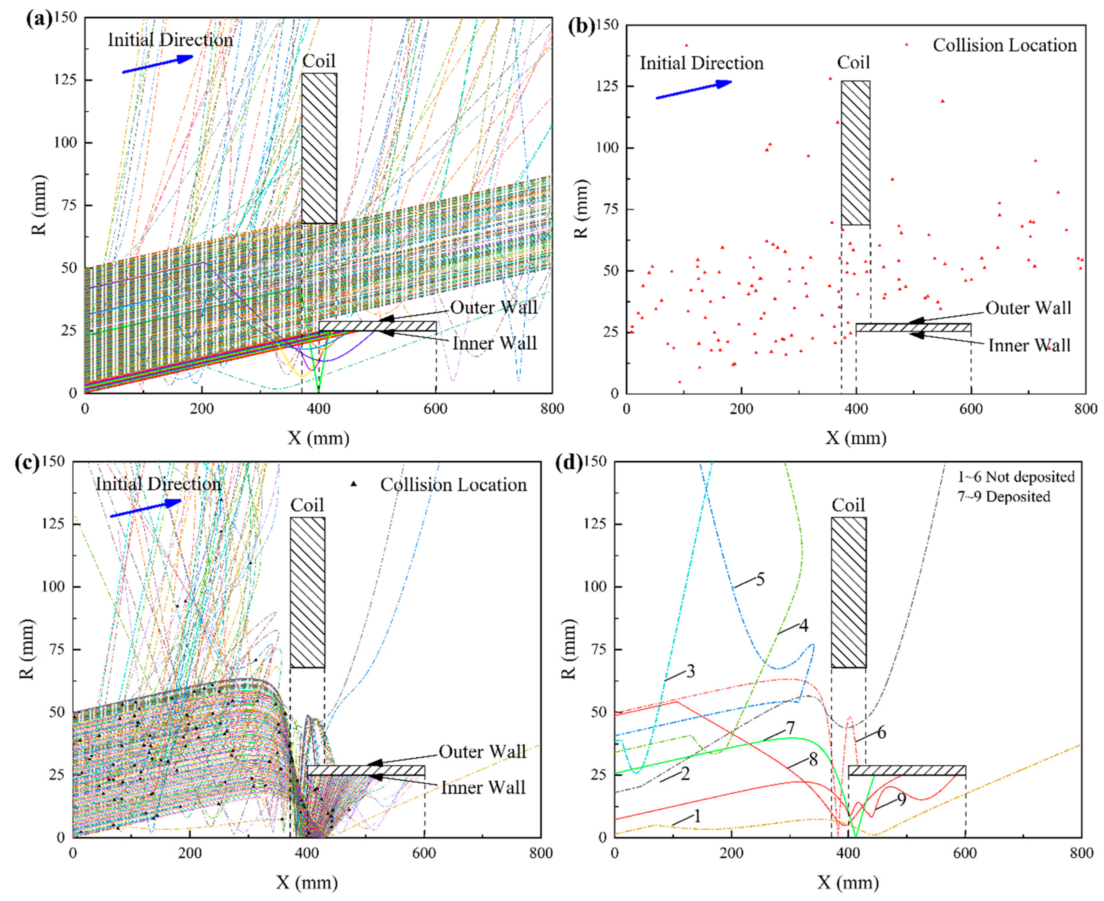
3.2.2. Effect of Magnetic Field on the Motion of Ions with Various Emission Angles

For ions with various emission angles, the effect of the magnetic field was also investigated. An emission angle of 3° was chosen so that with the geometric relation, some of the ions could move directly onto the inner surface of the pipe, which could represent the actual process to some extent. Figure 9 shows the trajectories of the ions without a magnetic field. Most ions could not deposit on the inner surface except the ions with R < 3 mm. Ions with R > 45 mm were blocked by the coil surface.

Figure 10 shows the trajectories of the ions under different characteristic magnetic flux densities. When the characteristic magnetic flux density was relatively small (230 Gs), similar to the case without a magnetic field, only the ions emitted from the arc source with small R (<3 mm) could deposit onto the area near the inlet of the pipe (Figure 10a). As the characteristic magnetic flux density increased to 690 Gs, the ions were either blocked by the pipe or moved through the pipe (Figure 10b). With an increase in the characteristic magnetic flux density, the ions began to deposit after a returning motion towards the center axis (Figure 10c). Some ions with R > 45 mm were close to the coil, gaining a larger Lorentz force, and would move over the inlet of the pipe and deposit on the inner surface, increasing the deposition depth (Figure 10d).

With a further increase in the characteristic magnetic flux density, the ions turned to form a continual trajectory, with fewer ions blocked by the pipe (Figure 10e,f). As the characteristic magnetic flux density increased to 1610 Gs, the number of deposited ions reached a maximum value. With the characteristic magnetic flux density increasing to 3450 Gs, the returning motion made some ions deposit at the outlet of the pipe (Figure 10g). Even though a few ions (R > 41 mm) moved away from the pipe under the Lorentz force near the coil, most ions could deposit, which had a similarity with the 1840 Gs case. With the characteristic magnetic flux density increasing to 4600 Gs, the motion of multiple returning ions caused fewer ions to deposit (Figure 10h). Besides, more ions were deflected away from the pipe. Therefore, if the characteristic magnetic flux density continued to increase, more ions would move away from the pipe or through the pipe, which was unbeneficial for inner surface deposition. The trend of the number of deposited ions demonstrated a periodicity.

Figure 11 shows the deposition distance from the pipe inlet under different characteristic magnetic flux densities. Generally, the deposition depth decreased with an increase in the emission radius. Under a low characteristic magnetic flux density (less than 1380 Gs), ion deposition occurred only at the outlet and inlet areas of the pipe. With an increase in the characteristic magnetic flux density, the distribution became continual and gradually shifted towards the inlet of the pipe. As the characteristic magnetic flux density kept increasing to 4600 Gs, the returning motion would make some ions deposit back to the outlet of the pipe, resulting in an increase in the deposition depth. In addition, for different emission radii, the number of ions with returning motion could vary, causing the difference in the deposition depth.

Figure 12 shows the deposition distance from the pipe inlet of ions with the emission angle α under the characteristic magnetic flux density 1840 Gs. The deposition depth decreased with an increase in α. For the same α, the deposition depth decreased with an increase in the emission radius. Based on the model developed for the horizontally emitted ions (Equation (10)), an extended model considering the influence of the emission angle was developed as shown in Equation (11).

$$D=D_B{e}^{-B/B_0}+D_R{e}^{-R/R_0}-D_{\mathsf{\alpha }}\mathsf{\alpha }$$

(11)

Herein, D_α (unit: mm/°) is the average value of the slopes of the fitting lines. When α = 0, Equation (11) becomes Equation (10). This extended model provides the relationship between the deposition depth and magnetic field, the emission angle and the emission position of the ions. By using the model, the deposition depth of the ions with various emission angles and emission positions could be predicted.

3.2.3. Effect of Magnetic Field on Deposition Ratio

To describe the percentage of ions that deposited on the inner surface of the pipe in the study, an index named the deposition ratio was defined. Figure 13 shows the relationship between the deposition ratio and the characteristic magnetic flux density. For different emission angles α, the application of the magnetic field significantly influenced the deposition ratio. Under the effect of the periodic returning motion of the ions towards the center axis, the deposition ratio showed multiple peaks, while the peak value decreased with an increase in the characteristic magnetic flux density. Besides, further increasing the intensity reduced the deposition ratio.

3.3. Influence of Ion-Neutral Collision

To investigate the influence of the elastic scattering, the collision of the ions and gas was considered in the simulation. A comparison of the ions’ trajectories with an emission angle of 3° was conducted between the characteristic magnetic flux densities 0 and 1840 Gs (Figure 14). After collisions, some ions changed direction within their original plane; others gained velocities perpendicular to the original plane. Hence, their distances to the axis (R) showed folded lines or conic curves in the trajectories. Without a magnetic field, the proportion of collisions was 40% (10 of 25 ions, Figure 14a). Six ions collided with gas in the region between the source and the pipe inlet. Under a characteristic magnetic flux density of 1840 Gs, the ions had relatively longer flight times. Therefore, seven collisions occurred in the region between the source and pipe inlet (Figure 14b). Because most ions were guided inside the pipe and deposited in a short period of time, one collision happened inside the pipe. As for the ions that did not encounter collisions, their trajectories were the same as the cases shown in Figure 9 and Figure 10.

To reduce the contingency caused by the limit of the ions number used before, a simulation of ion motion was conducted with an ion emission density 10 times higher. The same comparison was carried out between the cases of 0 Gs (Figure 15a,b) and 1840 Gs (Figure 15c,d). The dash-dotted lines represent the trajectories of the ions that did not deposit inside the pipe, and the solid lines represent the trajectories of the ions that could deposit inside the pipe. The collision locations in Figure 15b,c show that the collisions were uniformly distributed in the path of the ion flux. A few collisions happened outside the main ion flux because some ions were scattered away from their original directions and collided with gas again. In the region between the source and the pipe inlet, the collision proportion was 32% for 0 Gs and 35.6% for 1840 Gs.

To break down the motion of the ions under the co-effect of the collision and magnetic field, Figure 15d shows nine typical trajectories extracted from Figure 15c. In Trajectories 1–4, the collisions happened relatively far from the pipe. Ions could move through the pipe (1), move through the hole of the coil (2), get reflected by the magnetic field (3) or move away from the coil (4). Trajectory 5 shows the collision near the coil and the reflection under the magnetic mirror effect. For Trajectories 6 and 7, the ions did not collide with gas and deposited on the outer and inner wall of the pipe, respectively. Trajectory 8 shows the collision outside the pipe to make the ion deposit on the inner wall, and Trajectory 9 provides an example of collisions inside the pipe to increase the deposition depth.

The influence of collisions lies in the combination of two processes. In Figure 15a, 5 of 250 ions turned to deposit inside the pipe after collisions and increased the deposition depth, and 6 of 250 ions were deflected away from the original routine and could not deposit. Hence, the deposition ratio dropped from 8% to 7.6% compared to what is shown in Figure 9. Under a characteristic magnetic flux density of 1840 Gs, two ions turned to deposit inside the pipe after collisions, while 54 ions moved away from the pipe (Figure 15c). Therefore, the deposition ratio dropped from 92% to 71.2% compared to what is shown in Figure 10f. The decrease in the deposition ratio was explained by Aksenov et al. [57], Eriksson et al. [58] and Goldberg et al. [59], using the reason that collision with background gas limits the ion density towards the substrate. In this study, ions that were affected by elastic collisions would either move into the pipe to deposit, or away from the pipe. The proportion of the ions moving into the pipe was relatively lower. Even though the deposition ratio decreased due to the influence of collision, the ratio was improved with the magnetic field. Additionally, the distribution of the deposition depth generally maintained similarity with the cases without collision. Hence, the application of a magnetic field can still improve the deposition ratio and depth.

4. Conclusions

In this study, a simulation of magnetic-field-induced ion motion in vacuum arc deposition for the inner surfaces of a tubular workpiece was performed. The influence of a magnetic field on ion motion was simulated. The effect of the magnetic field on ion trajectory motion was studied, and several conclusions can be drawn as follows.

• The trajectories of ions can be controlled via a magnetic field, and the ions can be deposited at different positions on the inner surface of the pipe by adjusting the magnetic flux density. The deposition ratio of the ions is low at low magnetic flux densities, and increases to a maximum value with an increase in the magnetic flux density. Further increasing the magnetic flux density leads to periodicity in the ions’ trajectories and the deposition ratio.
• The deposition depth of ions can be controlled by the magnetic flux density, ion emission radius and emission angle. When the magnetic flux density is relatively high, the deposition depth decreases as an exponential function of the magnetic flux density and ion emission radius, respectively. With an increase in the emission angle, the deposition depth decreases linearly. A numerical model was proposed to express the distribution of the deposition depth.
• The deposition efficiency and the depth of the inner surface can be improved by a magnetic field in an environment with a certain density of neutral gas. Ions that are affected by elastic collisions would either move into the pipe to deposit, or away from the pipe. The proportion of the ions moving into the pipe is relatively lower than that of ions moving away from the pipe.

References

1. Wei, R.; Rincon, C.; Booker, T.L.; Arps, J.H. Magnetic field enhanced plasma (MFEP) deposition of inner surfaces of tubes. Surf. Coat. Technol. 2004, 188–189, 691–696. [Google Scholar] [CrossRef]
2. Wen, X.Q.; Wang, J. Deposition of diamond-like carbon films on the inner surface of narrow stainless steel tubes. Vacuum 2010, 85, 34–38. [Google Scholar] [CrossRef]
3. Lusk, D.; Gore, M.; Boardman, W.; Casserly, T.; Boinapally, K.; Oppus, M.; Upadhyaya, D.; Tudhope, A.; Gupta, M.; Cao, Y.; et al. Thick DLC films deposited by PECVD on the internal surface of cylindrical substrates. Diam. Relat. Mater. 2008, 17, 1613–1621. [Google Scholar] [CrossRef] [Green Version]
4. Hatada, R.; Flege, S.; Bobrich, A.; Ensinger, W.; Dietz, C.; Baba, K.; Sawase, T.; Watamoto, T.; Matsutani, T. Preparation of Ag-containing diamond-like carbon films on the interior surface of tubes by a combined method of plasma source ion implantation and DC sputtering. Appl. Surf. Sci. 2014, 310, 257–261. [Google Scholar] [CrossRef]
5. Tian, X.B.; Jiang, H.F.; Gong, C.Z.; Yang, S.Q.; Fu, R.K.Y.; Chu, P.K. DLC deposition inside tubes using hollow cathode discharge plasma immersion ion implantation and deposition. Surf. Coat. Technol. 2010, 204, 2909–2912. [Google Scholar] [CrossRef]
6. Lozovan, A.A.; Alexandrova, S.S.; Mishnev, M.A.; Prishepov, S.V. A study of the deposition process of multilayer coatings on the inner tube surface with the pulsed laser deposition technique. J. Alloys Compd. 2014, 586, S387–S390. [Google Scholar] [CrossRef]
7. Baba, K.; Hatada, R.; Flege, S.; Ensinger, W. DLC coating of interior surfaces of steel tubes by low energy plasma source ion implantation and deposition. Appl. Surf. Sci. 2014, 310, 262–265. [Google Scholar] [CrossRef]
8. Kawasaki, H.; Nishiguchi, H.; Furutani, T.; Ohshima, T.; Yagyu, Y.; Ihara, T.; Shinohara, M.; Suda, Y. Coating of inner surface of cylindrical pipe for hydrogen entry prevention using plasma process. Jpn. J. Appl. Phys. 2018, 57, 01AB02. [Google Scholar] [CrossRef] [Green Version]
9. Anders, A. A review comparing cathodic arcs and high power impulse magnetron sputtering (HiPIMS). Surf. Coat. Technol. 2014, 257, 308–325. [Google Scholar] [CrossRef] [Green Version]
10. Shi, C.L.; Zhang, M.; Lin, G.Q. Effect of pulsed bias on tin film deposition on internal wall of deep tubes by arc ion plating. Chin. J. Vac. Sci. Technol. 2007, 27, 517–521. [Google Scholar] [CrossRef]
11. Boxman, R.L.; Beilis, I.I.; Gidalevich, E.; Zhitomirsky, V.N. Magnetic control in vacuum arc deposition: A review. IEEE Trans. Plasma Sci. 2005, 33, 1618–1625. [Google Scholar] [CrossRef]
12. Beilis, I.I.; Sagi, B.; Zhitomirsky, V.; Boxman, R.L. Cathode spot motion in a vacuum arc with a long roof-shaped cathode under magnetic field. J. Appl. Phys. 2015, 117, 233303. [Google Scholar] [CrossRef]
13. Benilov, M.S.; Kaufmann, H.T.C.; Hartmann, W.; Benilova, L.G. Revisiting Theoretical Description of the Retrograde Motion of Cathode Spots of Vacuum Arcs. IEEE Trans. Plasma Sci. 2019, 47, 3434–3441. [Google Scholar] [CrossRef]
14. Chaar, A.B.B.; Syed, B.; Hsu, T.; Johansson-Jöesaar, M.; Andersson, J.M.; Henrion, G.; Johnson, L.J.S.; Mücklich, F.; Odén, M. The Effect of Cathodic Arc Guiding Magnetic Field on the Growth of (Ti0.36Al0.64)N Coatings. Coatings 2019, 9, 660. [Google Scholar] [CrossRef] [Green Version]
15. Giuliani, L.; Minotti, F.; Grondona, D.; Kelly, H. On the Dynamics of the Plasma Entry and Guiding in a Straight Magnetized Filter of a Pulsed Vacuum Arc. IEEE Trans. Plasma Sci. 2007, 35, 1710–1716. [Google Scholar] [CrossRef]
16. Wang, S.; Lin, Z.; Qiao, H.; Ba, D.; Zhu, L. Influence of a Scanning Radial Magnetic Field on Macroparticle Reduction of Arc Ion-Plated Films. Coatings 2018, 8, 49. [Google Scholar] [CrossRef] [Green Version]
17. Paperny, V.L.; Krasov, V.I.; Lebedev, N.V.; Astrakchantsev, N.V.; Chernikch, A.A. Vacuum arc plasma mass separator. Plasma Sources Sci. Technol. 2014, 24, 15009. [Google Scholar] [CrossRef]
18. Zhang, G.L.; Wang, J.L.; Wu, X.F.; Feng, W.R.; Chen, G.L.; Gu, W.C.; Niu, E.W.; Fan, S.H.; Liu, C.Z.; Yang, S.Z. Inner Surface Modification of a Tube by Magnetic Glow-Arc Plasma Source Ion Implantation. Chin. Phys. Lett. 2006, 23, 1241–1244. [Google Scholar] [CrossRef]
19. Aksenov, I.I.; Khoroshikh, V.M.; Belous, V.A.; Leonov, S.A. Vacuum-arc systems for depositing drop-free coatings onto inner surfaces. Mater. Sci. Forum 1998, 287–288, 287–290. [Google Scholar] [CrossRef]
20. Liu, Q.; Wang, W.T.; Lin, G.Q. Magnetic field and tin film growth by arc ion plating on inner walls of deep tubes. Chin. J. Vac. Sci. Technol. 2011, 31, 71–75. [Google Scholar] [CrossRef]
21. Arustamov, V.N.; Ashurov, K.B.; Kadirov, K.K.; Khudaykulov, I.K. Formation of technological plasma effect of vacuum-arc discharge on inner surface of metallic pipes and deposition of protective coats on them. In Proceedings of the 13th International Conference on Plasma Surface Engineering, Garmisch-Partenkirchen, Germany, 10–14 September 2012. [Google Scholar]
22. Lang, W.C.; Gao, B.; Nan, X.R. Process Development of Films Deposited on Inner Wall of Long Tube by Arc Ion Plating. Appl. Mech. Mater. 2012, 152–154, 1705–1710. [Google Scholar] [CrossRef]
23. Zhao, Y.; Guo, C.; Yang, W.; Chen, Y.; Yu, B. TiN films deposition inside stainless-steel tubes using magnetic field-enhanced arc ion plating. Vacuum 2015, 112, 46–54. [Google Scholar] [CrossRef]
24. Kostrin, D.K.; Lisenkov, A.A. Plasmachemical synthesis of coatings using a vacuum arc discharge. Vak. Forsch. Prax. 2017, 29, 35–39. [Google Scholar] [CrossRef]
25. Birdsall, C.K.; Langdon, A.B. Plasma Physics via Computer Simulation, 1st ed.; McGraw-Hill: New York, NY, USA, 1991; pp. 27–47. [Google Scholar]
26. Skullerud, H.R. The stochastic computer simulation of ion motion in a gas subjected to a constant electric field. J. Phys. D Appl. Phys. 1968, 1, 1567–1568. [Google Scholar] [CrossRef]
27. Li, H.; Sun, L.; Wu, G.; Dai, W.; Zhou, Y.; Wang, A.Y. Simulation of magnetic field distribution in doubly-bent filter cathode of vacuum arc film growth setup. Chin. J. Vac. Sci. Technol. 2010, 30, 614–620. [Google Scholar] [CrossRef]
28. Takahashi, K.; Uchino, T.; Ikegami, K.; Sasaki, T.; Kikuchi, T.; Harada, N. Behavior of Laser Ablation Plasma During Transport in Multicusp Magnetic Field Using Different Targets for Laser Ion Source. Energy Procedia 2017, 131, 354–358. [Google Scholar] [CrossRef]
29. Kanaya, K.; Kawakatsu, H. Secondary electron emission due to primary and backscattered electrons. J. Phys. D Appl. Phys. 1972, 5, 1727–1742. [Google Scholar] [CrossRef]
30. Jin, J.M. The Finite Element Method in Electromagnetics, 3rd ed.; John Wiley & Sons: New York, NY, USA, 2014; pp. 10–52. [Google Scholar]
31. Chung, J.; Hulbert, G.M. A time integration algorithm for structural dynamics with improved numerical dissipation: The generalized-α method. J. Appl. Mech. 1993, 60, 371–375. [Google Scholar] [CrossRef]
32. Lieberman, M.A.; Lichtenberg, A.J. Principles of Plasma Discharges and Materials Processing, 2nd ed.; John Wiley & Sons: New York, NY, USA, 2005; pp. 157–167. [Google Scholar]
33. Li, Y.; Jing, X.; Yuan, Q.; Li, J. Numerical Analysis of Magnetized Sheath for Inner Surface Modification. IEEE Access 2019, 7, 53147–53151. [Google Scholar] [CrossRef]
34. Hershkowitz, N. Sheaths: More complicated than you think. Phys. Plasmas 2005, 12, 55502. [Google Scholar] [CrossRef]
35. Baalrud, S.D. Influence of ion streaming instabilities on transport near plasma boundaries. Plasma Sources Sci. Technol. 2016, 25, 25008. [Google Scholar] [CrossRef] [Green Version]
36. Bohm, D. Minimum ionic kinetic energy for a stable sheath. In The Characteristics of Electrical Discharges in Magnetic Fields, 1st ed.; Guthry, A., Wakerling, R.K., Eds.; McGraw-Hill: New York, NY, USA, 1949; Volume 144, pp. 209–250. [Google Scholar]
37. Chodura, R. Plasma-wall transition in an oblique magnetic field. Phys. Fluids 1982, 25, 1628. [Google Scholar] [CrossRef] [Green Version]
38. Kim, G.H.; Hershkowitz, N.; Diebold, D.A.; Cho, M.H. Magnetic and collisional effects on presheaths. Phys. Plasmas 1995, 2, 3222–3233. [Google Scholar] [CrossRef]
39. Aksenov, I.I.; Strel’Nitskij, V.E.; Vasilyev, V.V.; Zaleskij, D.Y. Efficiency of magnetic plasma filters. Surf. Coat. Technol. 2003, 163–164, 118–127. [Google Scholar] [CrossRef]
40. Ristivojevic, Z.; Petrović, Z.L. A Monte Carlo simulation of ion transport at finite temperatures. Plasma Sources Sci. Technol. 2012, 21, 35001. [Google Scholar] [CrossRef] [Green Version]
41. Astley, R.J. Infinite elements for wave problems: A review of current formulations and an assessment of accuracy. Int. J. Numer. Meth. Eng. 2000, 49, 951–976. [Google Scholar] [CrossRef]
42. Burnett, D.S. A three-dimensional acoustic infinite element based on a prolate spheroidal multipole expansion. J. Acoust. Soc. Am. 1994, 96, 2798–2816. [Google Scholar] [CrossRef]
43. Jüttner, B. Cathode spots of electric arcs. J. Phys. D Appl. Phys. 2001, 34, R103–R123. [Google Scholar] [CrossRef]
44. Kutzner, J.; Miller, H.C. Integrated ion flux emitted from the cathode spot region of a diffuse vacuum arc. J. Phys. D Appl. Phys. 1992, 25, 686–693. [Google Scholar] [CrossRef]
45. Byon, E.; Anders, A. Ion energy distribution functions of vacuum arc plasmas. J. Appl. Phys. 2003, 93, 1899–1906. [Google Scholar] [CrossRef] [Green Version]
46. Boxman, R.L.; Sanders, D.; Martin, P. Handbook of Vacuum arc Science and Technology, 1st ed.; NOYES Publications: Parkridge, NJ, USA, 1995; pp. 151–256. [Google Scholar]
47. Aksenov, I.I.; Khoroshikh, V.M. Angular distributions of ions in a plasma stream of a steady-state vacuum arc. In Proceedings of the ISDEIV 18th International Symposium on Discharges and Electrical Insulation in Vacuum, Eindhoven, The Netherlands, 1 January 1998. [Google Scholar] [CrossRef]
48. Anders, A.; Yushkov, G.Y. Angularly resolved measurements of ion energy of vacuum arc plasmas. Appl. Phys. Lett. 2002, 80, 2457–2459. [Google Scholar] [CrossRef] [Green Version]
49. Heberlein, J.V.R.; Porto, D.R. The Interaction of Vacuum Arc Ion Currents with Axia I Magnetic Fields. IEEE Trans. Plasma Sci. 1983, 3, 152–159. [Google Scholar] [CrossRef]
50. Purcell, E.M. Electricity and Magnetism, 2nd ed.; McGraw-Hill: New York, NY, USA, 1985; pp. 226–231. [Google Scholar]
51. Cohen, S.A.; Siefert, N.S.; Stange, S.; Boivin, R.F.; Scime, E.E.; Levinton, F.M. Ion acceleration in plasmas emerging from a helicon-heated magnetic-mirror device. Phys. Plasmas 2003, 10, 2593–2598. [Google Scholar] [CrossRef] [Green Version]
52. Boercker, D.B.; Sanders, D.M.; Storer, J.; Falabella, S. Modeling plasma flow in straight and curved solenoids. J. Appl. Phys. 1991, 69, 115–120. [Google Scholar] [CrossRef]
53. Cluggish, B.P. Transport of a cathodic arc plasma in a straight, magnetized duct. IEEE Trans. Plasma Sci. 1998, 26, 1645–1652. [Google Scholar] [CrossRef]
54. Kelly, H.; Giuliani, L.; Rausch, F. Characterization of the ion emission in a pulsed vacuum arc with an axial magnetic field. J. Phys. D Appl. Phys. 2003, 36, 1980–1986. [Google Scholar] [CrossRef]
55. Zhitomirsky, V.N.; Zarchin, O.; Boxman, R.L.; Goldsmith, S. Transport of a vacuum arc produced plasma beam in a magnetized cylindrical duct. IEEE Trans. Plasma Sci. 2003, 31, 977–982. [Google Scholar] [CrossRef]
56. Nagelkerke, N.J.D. A Note on a General Definition of the Coefficient of Determination. Biometrika 1991, 78, 691–692. [Google Scholar] [CrossRef]
57. Eriksson, A.O.; Mraz, S.; Jensen, J.; Hultman, L.; Zhirkov, I.; Schneider, J.M.; Rosen, J. Influence of Ar and N2 Pressure on Plasma Chemistry, Ion Energy, and Thin Film Composition During Filtered Arc Deposition From Ti3SiC2 Cathodes. IEEE Trans. Plasma Sci. 2014, 42, 3498–3507. [Google Scholar] [CrossRef]
58. Aksenov, I.I.; Belous, V.A.; Zadneprovskiy, Y.A.; Kuprin, A.S.; Lomino, N.S.; Ovcharenko, V.D.; Sobol, O.V. Influence of Nitrogen Pressure on Silicon Content in Ti-Si-N Coatings Deposited by the Vacuum-Arc Method. In Proceedings of the XXIVth Int. Symp. on Discharges and Electrical Insulation in Vacuum, Braunschweig, Germany, 30 August–3 September 2010. [Google Scholar] [CrossRef]
59. Goldberg, O.; Goldenberg, E.; Zhitomirsky, V.N.; Cohen, S.R.; Boxman, R.L. Zirconium vacuum arc operation in a mixture of Ar and O2 gases: Ar effect on the arcing characteristics, deposition rate and coating properties. Surf. Coat. Technol. 2012, 206, 4417–4424. [Google Scholar] [CrossRef]
Figure 1. Schematic diagram of the vacuum arc deposition for the inner surface of a pipe.
Coatings 10 01053 g001
Figure 2. Mesh configuration: (a) General view of the mesh; (b) Detailed mesh of the arc source, coil and pipe.
Coatings 10 01053 g002
Figure 3. Schematic diagram of ion’s initial velocity direction.
Coatings 10 01053 g003
Figure 4. Simulation result for magnetic field distribution with coil current of 7.5A: (a) Field distribution with color bar (unit: Gs) in XR cross-section; (b) Magnetic flux density along X-axis; (c) Magnetic flux density along R-direction in a center plane (X = 400 mm).
Coatings 10 01053 g004
Figure 5. The linear relationship between the simulated characteristic magnetic flux density and coil current.
Coatings 10 01053 g005
Figure 6. Trajectories of horizontally emitted ions with different emission radii under no magnetic field.
Coatings 10 01053 g006
Figure 7. Trajectories of horizontally emitted ions with different characteristic magnetic flux densities: (a) 230 Gs; (b) 690 Gs; (c) 920 Gs; (d) 977 Gs; (e) 1840 Gs; (f) 2622 Gs; (g) 3450 Gs; (h) 4600 Gs.
Coatings 10 01053 g007aCoatings 10 01053 g007b
Figure 8. Distance from the pipe inlet of deposited ions with emission radius.
Coatings 10 01053 g008
Figure 9. Trajectories of ions with emission angle of 3° under no magnetic field.
Coatings 10 01053 g009
Figure 10. Trajectories of ions with emission angle of 3° under characteristic magnetic flux densities: (a) 230 Gs; (b) 690 Gs; (c) 1092 Gs; (d) 1380 Gs; (e) 1610 Gs; (f) 1840 Gs; (g) 3450 Gs; (h) 4600 Gs.
Coatings 10 01053 g010aCoatings 10 01053 g010b
Figure 11. The distance from the pipe inlet of deposited ions with emission angle of 3° under different characteristic magnetic flux densities.
Coatings 10 01053 g011
Figure 12. Variation of deposition distance from the pipe inlet of ions with emission angle α under the characteristic magnetic flux density of 1840 Gs.
Coatings 10 01053 g012
Figure 13. Relationship between deposition ratio and characteristic magnetic flux density for ions with various emission angles.
Coatings 10 01053 g013
Figure 14. Influence of ion-neutral elastic collision on the trajectories of ions under different characteristic magnetic flux densities: (a) 0 Gs; (b) 1840 Gs.
Coatings 10 01053 g014
Figure 15. Influence of elastic collision for a 10-times-higher ion number with different characteristic magnetic flux densities: (a) Ion trajectories in XR view (0 Gs); (b) Collision location distribution (0 Gs); (c) Ion trajectories in XR view with collision location (1840 Gs); (d) Typical trajectories of ions (1840 Gs).
Coatings 10 01053 g015