(R)evolution of the Standard Addition Procedure for Immunoassays


Abstract
:1. Introduction
2. Materials and Methods
2.1. Materials
2.2. Assay—Binding Inhibition Test
2.3. Simulation
2.4. RIfS Transducer Surface Modification
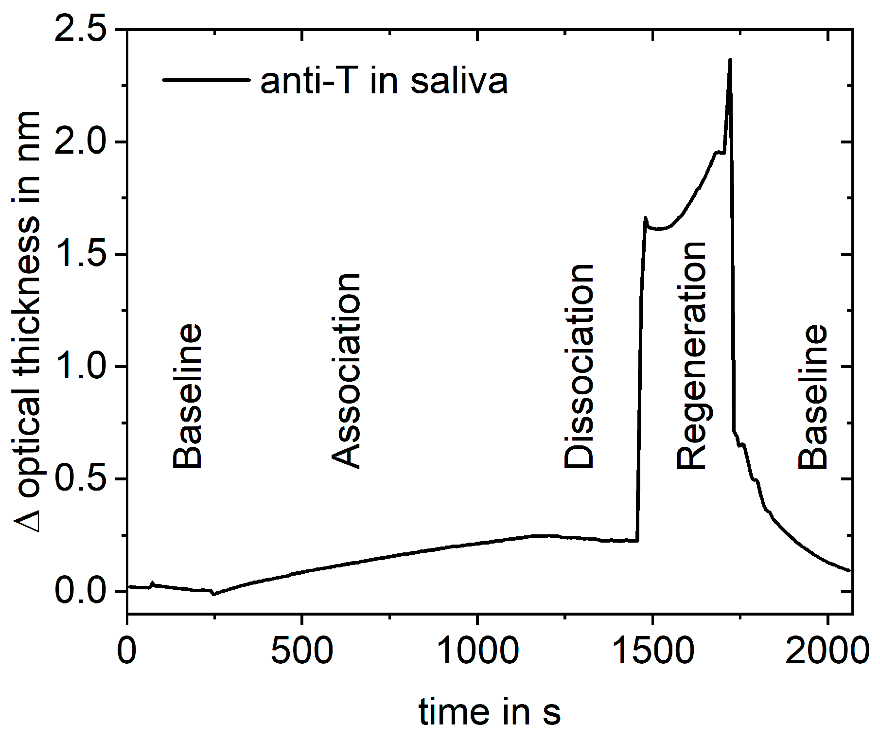
2.5. Reflectometric Interference Spectroscopy
2.6. RIfS Measurements
3. Results
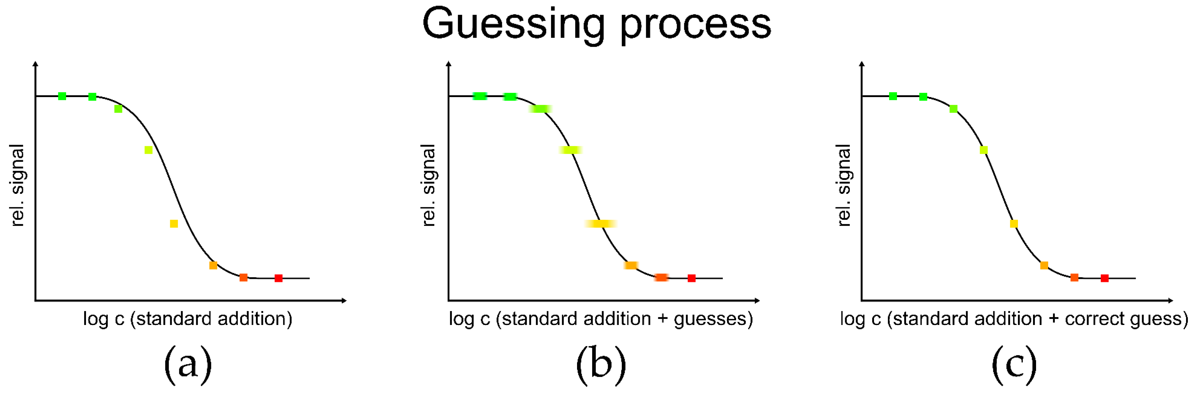
3.1. Simulations
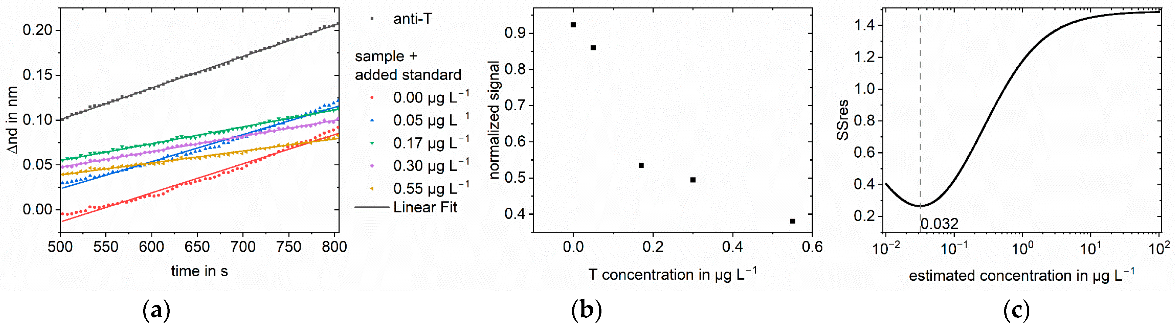
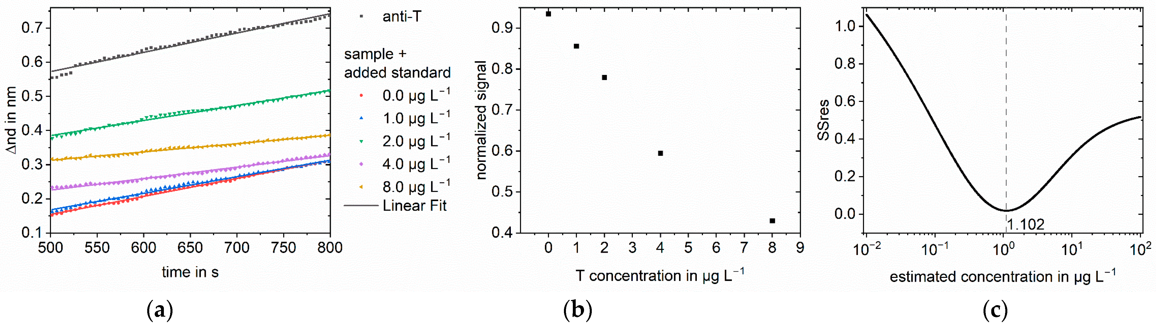
3.2. Measurements
4. Discussion
5. Conclusions
Author Contributions
Funding
Data Availability Statement
Conflicts of Interest
References
- Wang, K.; Lin, X.; Zhang, M.; Li, Y.; Luo, C.; Wu, J. Review of Electrochemical Biosensors for Food Safety Detection. Biosensors 2022, 12, 959. [Google Scholar] [CrossRef]
- Lavecchia, T.; Tibuzzi, A.; Giardi, M.T. Biosensors for functional food safety and analysis. Adv. Exp. Med. Biol. 2010, 698, 267–281. [Google Scholar] [CrossRef] [PubMed]
- Hashemi Goradel, N.; Mirzaei, H.; Sahebkar, A.; Poursadeghiyan, M.; Masoudifar, A.; Malekshahi, Z.V.; Negahdari, B. Biosensors for the Detection of Environmental and Urban Pollutions. J. Cell. Biochem. 2018, 119, 207–212. [Google Scholar] [CrossRef]
- Gavrilaș, S.; Ursachi, C.Ș.; Perța-Crișan, S.; Munteanu, F.-D. Recent Trends in Biosensors for Environmental Quality Monitoring. Sensors 2022, 22, 1513. [Google Scholar] [CrossRef]
- Connelly, J.T.; Baeumner, A.J. Biosensors for the detection of waterborne pathogens. Anal. Bioanal. Chem. 2012, 402, 117–127. [Google Scholar] [CrossRef]
- Gruhl, F.J.; Rapp, B.E.; Länge, K. Biosensors for diagnostic applications. Adv. Biochem. Eng. Biotechnol. 2013, 133, 115–148. [Google Scholar] [CrossRef]
- Zhang, Y.; Hu, Y.; Jiang, N.; Yetisen, A.K. Wearable artificial intelligence biosensor networks. Biosens. Bioelectron. 2022, 219, 114825. [Google Scholar] [CrossRef]
- Bhalla, N.; Jolly, P.; Formisano, N.; Estrela, P. Introduction to biosensors. Essays Biochem. 2016, 60, 1–8. [Google Scholar] [CrossRef] [PubMed]
- Sharma, S.; Byrne, H.; O’Kennedy, R.J. Antibodies and antibody-derived analytical biosensors. Essays Biochem. 2016, 60, 9–18. [Google Scholar] [CrossRef] [PubMed]
- Kaur, J.; Singh, P.K. Enzyme-based optical biosensors for organophosphate class of pesticide detection. Phys. Chem. Chem. Phys. 2020, 22, 15105–15119. [Google Scholar] [CrossRef]
- Newman, J.D.; Setford, S.J. Enzymatic biosensors. Mol. Biotechnol. 2006, 32, 249–268. [Google Scholar] [CrossRef]
- Fechner, P.; Gauglitz, G.; Gustafsson, J.-Å. Nuclear receptors in analytics—A fruitful joint venture or a wasteful futility? Trends Anal. Chem. 2010, 29, 297–305. [Google Scholar] [CrossRef]
- Tombelli, S.; Mascini, M. Aptamers biosensors for pharmaceutical compounds. Comb. Chem. High Throughput Screen. 2010, 13, 641–649. [Google Scholar] [CrossRef] [PubMed]
- Villalonga, A.; Pérez-Calabuig, A.M.; Villalonga, R. Electrochemical biosensors based on nucleic acid aptamers. Anal. Bioanal. Chem. 2020, 412, 55–72. [Google Scholar] [CrossRef]
- Andreasson, U.; Perret-Liaudet, A.; van Waalwijk Doorn, L.J.C.; Blennow, K.; Chiasserini, D.; Engelborghs, S.; Fladby, T.; Genc, S.; Kruse, N.; Kuiperij, H.B.; et al. A Practical Guide to Immunoassay Method Validation. Front. Neurol. 2015, 6, 179. [Google Scholar] [CrossRef] [PubMed]
- Wood, W.G. “Matrix Effects” in Immunoassays. Scand. J. Clin. Lab. Investig. 1991, 51, 105–112. [Google Scholar] [CrossRef]
- Oldfield, P.R. Understanding the matrix effect in immunoassays. Bioanalysis 2014, 6, 1425–1427. [Google Scholar] [CrossRef]
- Bader, M. A systematic approach to standard addition methods in instrumental analysis. J. Chem. Educ. 1980, 57, 703. [Google Scholar] [CrossRef]
- Hohn, H. Chemische Analysen mit dem Polarographen; Springer: Berlin, Germany, 1937. [Google Scholar]
- Harvey, C.E. Spectrochemical Procedures. Soil Sci. 1952, 74, 265. [Google Scholar] [CrossRef]
- Campbell, W.J.; Carl, H.F. Quantitative Analysis of Niobium and Tantalum in Ores by Fluorescent X-ray Spectroscopy. Anal. Chem. 1954, 26, 800–805. [Google Scholar] [CrossRef]
- Chow, T.J.; Thompson, T.G. Flame Photometric Determination of Strontium in Sea Water. Anal. Chem. 1955, 27, 18–21. [Google Scholar] [CrossRef]
- Kelly, W.R.; Pratt, K.W.; Guthrie, W.F.; Martin, K.R. Origin and early history of die Methode des Eichzusatzes or the Method of Standard Addition with primary emphasis on its origin, early design, dissemination, and usage of terms. Anal. Bioanal. Chem. 2011, 400, 1805–1812. [Google Scholar] [CrossRef] [PubMed]
- European Medicines Agency. ICH Guideline M10 on Bioanalytical Method Validation and Study Sample Analysis: EMA/CHMP/ICH/172948/2019, 2023. Available online: https://www.ema.europa.eu/en/ich-m10-bioanalytical-method-validation-scientific-guideline (accessed on 28 June 2023).
- Ellison, S.L.R.; Thompson, M. Standard additions: Myth and reality. Analyst 2008, 133, 992–997. [Google Scholar] [CrossRef]
- Findlay, J.W.A.; Dillard, R.F. Appropriate calibration curve fitting in ligand binding assays. AAPS J. 2007, 9, E260–E267. [Google Scholar] [CrossRef]
- Prinz, H. Hill coefficients, dose-response curves and allosteric mechanisms. J. Chem. Biol. 2010, 3, 37–44. [Google Scholar] [CrossRef]
- Goutelle, S.; Maurin, M.; Rougier, F.; Barbaut, X.; Bourguignon, L.; Ducher, M.; Maire, P. The Hill equation: A review of its capabilities in pharmacological modelling. Fundam. Clin. Pharmacol. 2008, 22, 633–648. [Google Scholar] [CrossRef] [PubMed]
- Weiss, J.N. The Hill equation revisited: Uses and misuses. FASEB J. 1997, 11, 835–841. [Google Scholar] [CrossRef]
- Abeliovich, H. An empirical extremum principle for the hill coefficient in ligand-protein interactions showing negative cooperativity. Biophys. J. 2005, 89, 76–79. [Google Scholar] [CrossRef]
- Pang, S.; Cowen, S. A generic standard additions based method to determine endogenous analyte concentrations by immunoassays to overcome complex biological matrix interference. Sci. Rep. 2017, 7, 17542. [Google Scholar] [CrossRef]
- Rau, S.; Gauglitz, G. Reflectometric interference spectroscopy (RIfS) as a new tool to measure in the complex matrix milk at low analyte concentration. Anal. Bioanal. Chem. 2012, 402, 529–536. [Google Scholar] [CrossRef]
- Conrad, M.; Fechner, P.; Proll, G.; Gauglitz, G. Comparison of methods for quantitative biomolecular interaction analysis. Anal. Bioanal. Chem. 2021, 414, 661–673. [Google Scholar] [CrossRef]
- Fechner, P.; Gauglitz, G.; Proll, G. Through the looking-glass—Recent developments in reflectometry open new possibilities for biosensor applications. Trends Anal. Chem. 2022, 156, 116708. [Google Scholar] [CrossRef]
- Gauglitz, G.; Brecht, A.; Kraus, G.; Nahm, W. Chemical and biochemical sensors based on interferometry at thin (multi-) layers. Sens. Actuators B Chem. 1993, 11, 21–27. [Google Scholar] [CrossRef]
- Cox, K.L.; Devanarayan, V.; Kriaucinas, A.; Manetta, J.; Montrose, C.; Sittampalam, S. Immunoassay Methods. In Assay Guidance Manual; Markossian, S., Grossman, A., Brimacombe, K., Arkin, M., Auld, D., Austin, C., Baell, J., Chung, T.D., Coussens, N.P., Dahlin, J.L., et al., Eds.; Eli Lilly & Company and the National Center for Advancing Translational Sciences: Bethesda, MD, USA, 2004. [Google Scholar]
- Yang, C.-Y.; Brooks, E.; Li, Y.; Denny, P.; Ho, C.-M.; Qi, F.; Shi, W.; Wolinsky, L.; Wu, B.; Wong, D.T.W.; et al. Detection of picomolar levels of interleukin-8 in human saliva by SPR. Lab Chip 2005, 5, 1017–1023. [Google Scholar] [CrossRef]
- Granger, D.A.; Shirtcliff, E.A.; Booth, A.; Kivlighan, K.T.; Schwartz, E.B. The “trouble” with salivary testosterone. Psychoneuroendocrinology 2004, 29, 1229–1240. [Google Scholar] [CrossRef]
- Morishita, M.; Aoyama, H.; Tokumoto, K.; Iwamoto, Y. The concentration of salivary steroid hormones and the prevalence of gingivitis at puberty. Adv. Dent. Res. 1988, 2, 397–400. [Google Scholar] [CrossRef]
- Vittek, J.; L’Hommedieu, D.G.; Gordon, G.G.; Rappaport, S.C.; Southren, A.L. Direct radioimmunoassay (RIA) of salivary testosterone: Correlation with free and total serum testosterone. Life Sci. 1985, 37, 711–716. [Google Scholar] [CrossRef]
- Mitchell, J.S.; Lowe, T.E. Ultrasensitive detection of testosterone using conjugate linker technology in a nanoparticle-enhanced surface plasmon resonance biosensor. Biosens. Bioelectron. 2009, 24, 2177–2183. [Google Scholar] [CrossRef]
- Mayo Clinic. TGRP—Overview: Testosterone, Total and Free, Serum. Available online: https://www.mayocliniclabs.com/test-catalog/overview/83686#Clinical-and-Interpretive (accessed on 7 July 2023).


| Matrix | Buffer | Milk | Saliva | Serum | ||||
|---|---|---|---|---|---|---|---|---|
| V in µL | v in µL s−1 | V in µL | v in µL s−1 | V in µL | v in µL s−1 | V in µL | v in µL s−1 | |
| Baseline | 100 | 0.4 | 240 | 2 | 60 | 0.5 | 100 | 0.5 |
| Association | 100 | 0.4 | 800 | 2 | 450 | 0.5 | 450 | 0.5 |
| Dissociation | 100 | 1 | 6000 | 20 | 360 | 2 | 1200 | 2 |
| 120 | 2 | |||||||
| Regeneration | 200 | 5 | 800 | 2 | 400 | 2 | 400 | 2 |
| Baseline | 150 | 0.4 | 300 | 2 | 100 | 0.5 | 100 | 0.5 |
| Method | Log-log | Logit-log | ||
|---|---|---|---|---|
| % Correct | M Correct Range | % Correct | M Correct Range | |
| 0.15 | 24 | 2.0 × 10⁻⁴–0.23 | 100 | 4.3 × 10⁻¹⁴–0.23 |
| 1.0 | 3 | 7.9 × 10⁻⁷–9.0 × 10⁻⁷ | 100 | 1.1 × 10⁻⁸–9.0 × 10⁻⁷ |
| 3.2 | 7 | 1.8 × 10⁻⁷–2.0 × 10⁻⁷ | 100 | 5.0 × 10⁻⁸–2.0 × 10⁻⁷ |
| Sample Concentration in µg L−1 | Analyte | Matrix | Found Concen-tration in µg L−1 Log-log | Recovery in % Log-log | Found Concen-tration in µg L−1 Logit-log | Recovery in % Logit-log | Improvement Factor |
|---|---|---|---|---|---|---|---|
| 3.0 | Testosterone | Buffer | 6.99 | 233 | 3.53 | 118 | 2 |
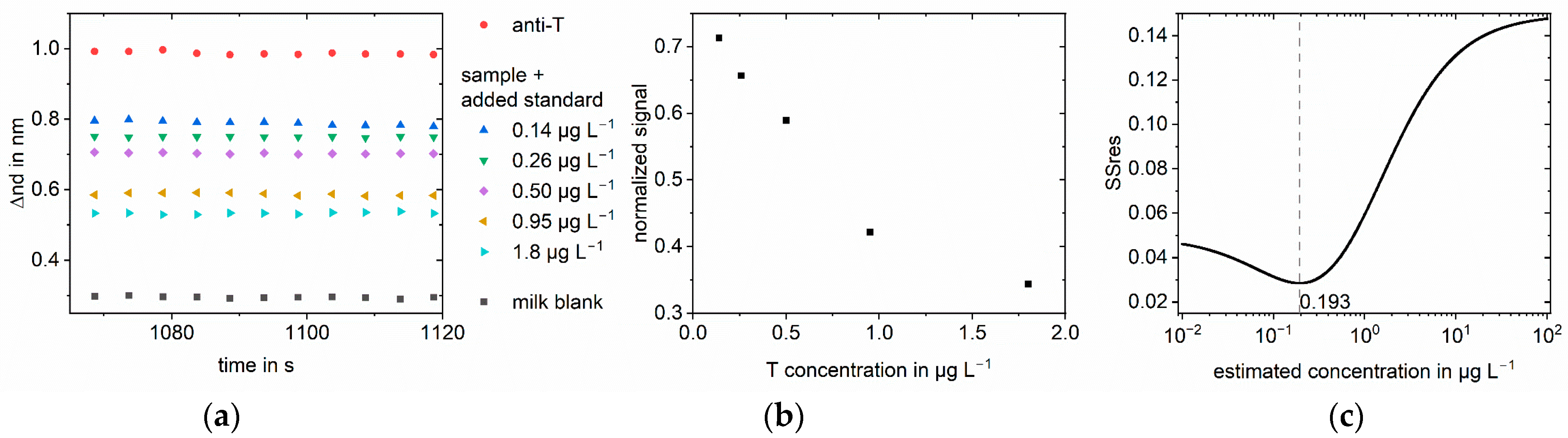
| 0.3 | Testosterone | Milk | 0.607 | 202 | 0.214 | 71 | 3 |
| 0.05 | Testosterone | Saliva | 0.124 | 249 | 0.035 | 70 | 4 |
| 1.0 | Testosterone | Serum | 187 | 18740 | 0.975 | 110 | 192 |
| 10 | Testosterone | Serum | - | - | 11.0 | 98 | ∞ |
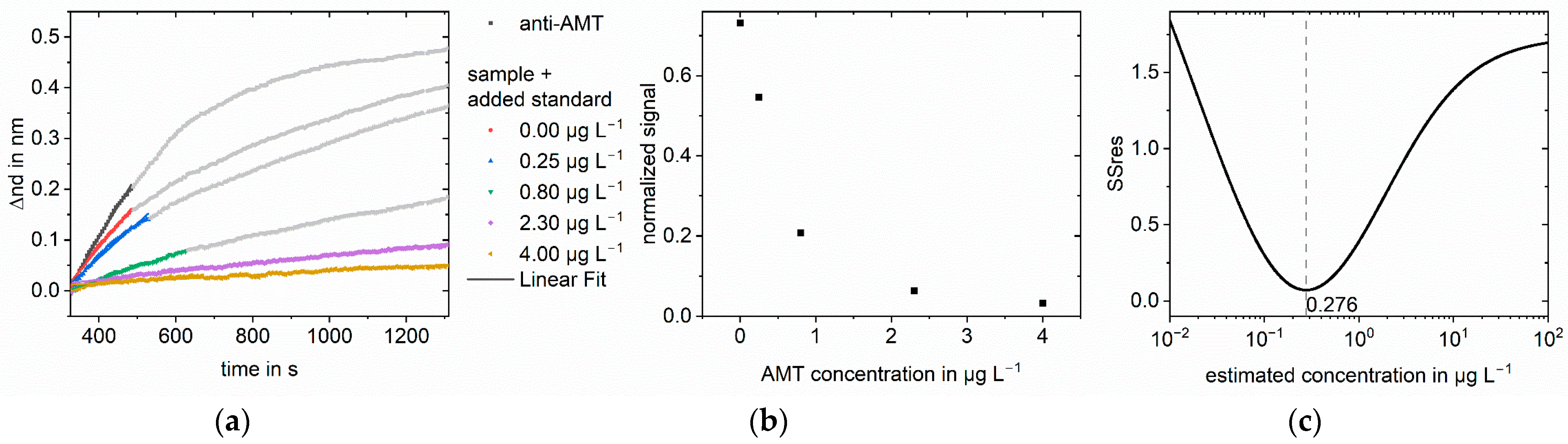
| 2.5 | Amitriptyline | Serum | 7.22 | 289 | 2.76 | 111 | 3 |
Disclaimer/Publisher’s Note: The statements, opinions and data contained in all publications are solely those of the individual author(s) and contributor(s) and not of MDPI and/or the editor(s). MDPI and/or the editor(s) disclaim responsibility for any injury to people or property resulting from any ideas, methods, instructions or products referred to in the content. |
© 2023 by the authors. Licensee MDPI, Basel, Switzerland. This article is an open access article distributed under the terms and conditions of the Creative Commons Attribution (CC BY) license (https://creativecommons.org/licenses/by/4.0/).
Share and Cite
Conrad, M.; Fechner, P.; Proll, G.; Gauglitz, G. (R)evolution of the Standard Addition Procedure for Immunoassays. Biosensors 2023, 13, 849. https://doi.org/10.3390/bios13090849
Conrad M, Fechner P, Proll G, Gauglitz G. (R)evolution of the Standard Addition Procedure for Immunoassays. Biosensors. 2023; 13(9):849. https://doi.org/10.3390/bios13090849
Chicago/Turabian StyleConrad, Monika, Peter Fechner, Günther Proll, and Günter Gauglitz. 2023. "(R)evolution of the Standard Addition Procedure for Immunoassays" Biosensors 13, no. 9: 849. https://doi.org/10.3390/bios13090849
APA StyleConrad, M., Fechner, P., Proll, G., & Gauglitz, G. (2023). (R)evolution of the Standard Addition Procedure for Immunoassays. Biosensors, 13(9), 849. https://doi.org/10.3390/bios13090849