
Enhancing Cutting Oil Efficiency with Nanoparticle Additives: A Gaussian Process Regression Approach to Viscosity and Cost Optimization

 , , , and
Abstract
1. Introduction
1.1. Motivation and Contributions
- •
- Bringing two measured and augmented datasets to the literature for different fluids.
- •
- Obtaining a reliable augmented dataset from measured values using Gaussian process regression.
- •
- Proposing a fitness function for the analysis of dynamic viscosity and nanofluid costs.
- •
- The most suitable nanofluid selection can be made with the proposed fitness function.
- •
- It provides scientific evidence for researchers on which nanofluid can be processed with high efficiency for which machining process, at which volumetric concentration, and at the most affordable cost.
1.2. Paper Organization
2. Materials and Methods
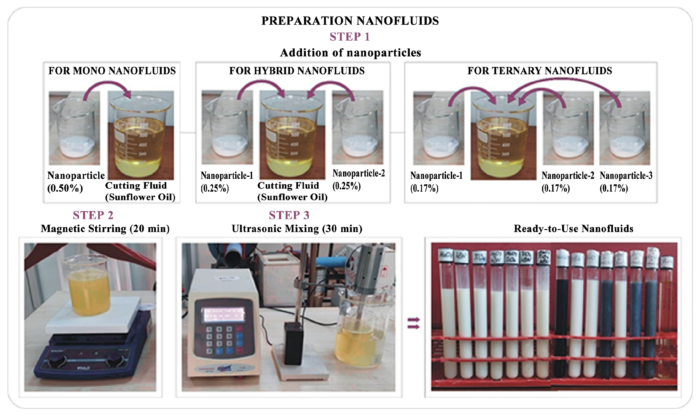
2.1. Nanofluid Preparation
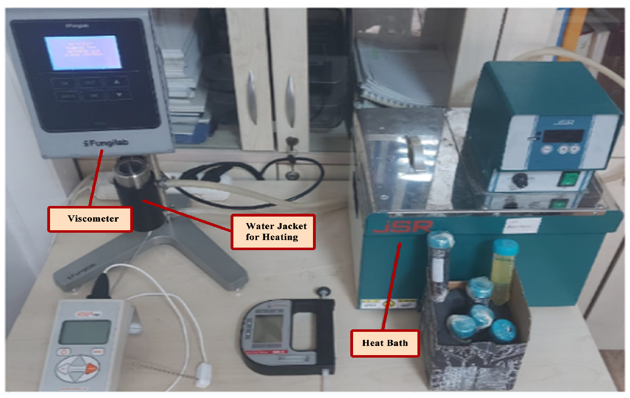
2.2. Viscosity Measurement
2.3. Dataset
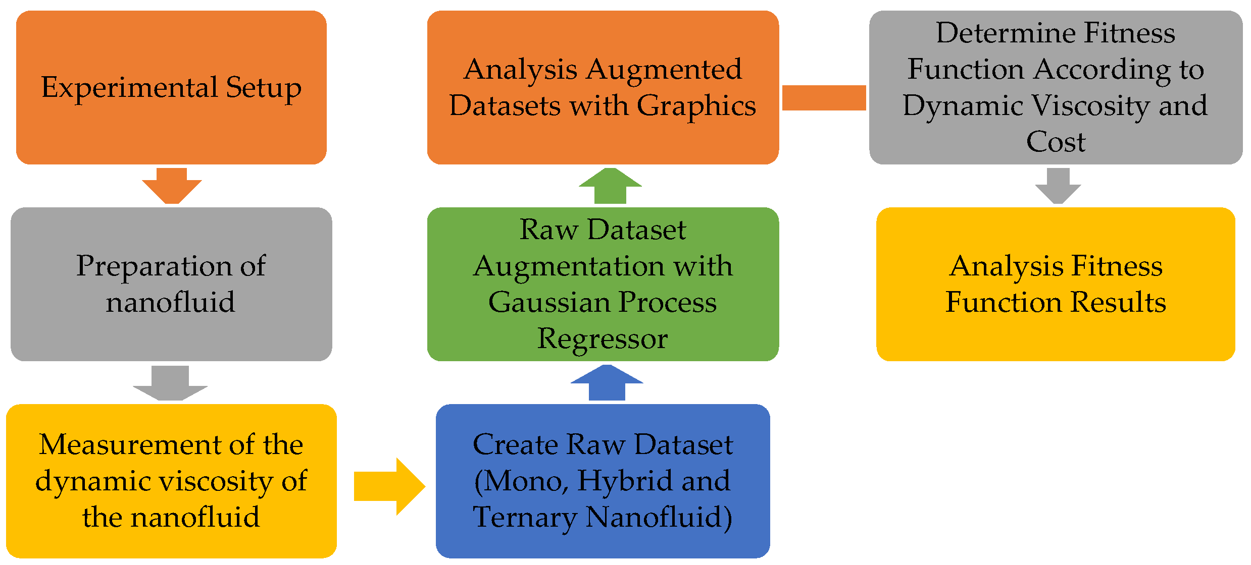
2.4. Our Method
2.5. Gaussian Process Regression (GPR)
- is the average function is taken as 0 in most cases.
- k (x, x′) = Cov (f(x), f(x′)) is the covariance function or kernel function.
- Gaussian Process Regression (GPR)
- Establishment of Joint Distribution
- Obtaining The Posterior Distribution
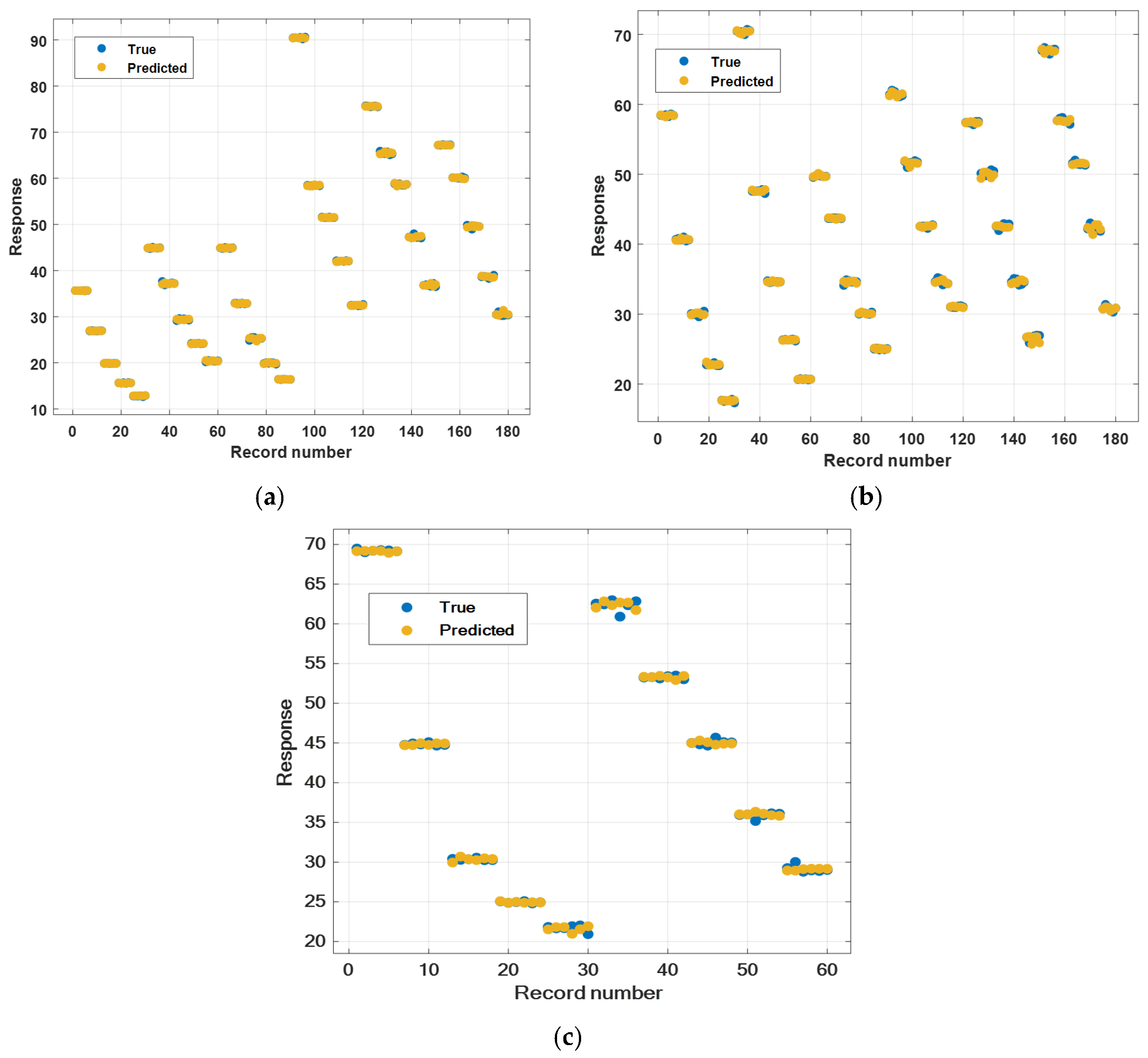
3. Experimental Results and Discussion
4. Conclusions
Author Contributions
Funding
Data Availability Statement
Conflicts of Interest
References
- Öndin, O.; Kıvak, T.; Sarıkaya, M.; Yıldırım, Ç.V. Investigation of the influence of MWCNTs mixed nanofluid on the machinability characteristics of PH 13-8 Mo stainless steel. Tribol. Int. 2020, 148, 106323. [Google Scholar] [CrossRef]
- Lee, J.-H.; Hwang, K.S.; Jang, S.P.; Lee, B.H.; Kim, J.H.; Choi, S.U.; Choi, C.J. Effective viscosities and thermal conductivities of aqueous nanofluids containing low volume concentrations of Al2O3 nanoparticles. Int. J. Heat Mass Transf. 2008, 51, 2651–2656. [Google Scholar] [CrossRef]
- Bag, R.; Panda, A.; Sahoo, A.K.; Kumar, R. A brief study on effects of nano cutting fluids in hard turning of AISI 4340 steel. Mater. Today Proc. 2020, 26, 3094–3099. [Google Scholar] [CrossRef]
- Ravi, S.; Gurusamy, P. Review of nanofluids as coolant in metal cutting operations. Mater. Today Proc. 2020, 37, 2387–2390. [Google Scholar] [CrossRef]
- Sharma, A.K.; Singh, R.K.; Dixit, A.R.; Tiwari, A.K. Novel uses of alumina-MoS2 hybrid nanoparticle enriched cutting fluid in hard turning of AISI 304 steel. J. Manuf. Process. 2017, 30, 467–482. [Google Scholar] [CrossRef]
- Yadav, R.; Dubey, V.; Sharma, A.K. Investigation of cutting forces in MQL turning using mono and hybrid nano cutting fluid. Mater. Today Proc. 2023; in press. [Google Scholar] [CrossRef]
- Gajrani, K.K.; Suvin, P.; Kailas, S.V.; Mamilla, R.S. Thermal, rheological, wettability and hard machining performance of MoS2 and CaF2 based minimum quantity hybrid nano-green cutting fluids. J. Mater. Process. Technol. 2019, 266, 125–139. [Google Scholar] [CrossRef]
- Selvarajoo, K.; Wanatasanappan, V.V.; Luon, N.Y. Experimental measurement of thermal conductivity and viscosity of Al2O3-GO (80:20) hybrid and mono nanofluids: A new correlation. Diam. Relat. Mater. 2024, 144, 111018. [Google Scholar] [CrossRef]
- Singh, R.K.; Sharma, A.K.; Dixit, A.R.; Tiwari, A.K.; Pramanik, A.; Mandal, A. Performance evaluation of alumina-graphene hybrid nano-cutting fluid in hard turning. J. Clean. Prod. 2017, 162, 830–845. [Google Scholar] [CrossRef]
- Hegab, H.; Darras, B.; Kishawy, H. Sustainability Assessment of Machining with Nano-Cutting Fluids. Procedia Manuf. 2018, 26, 245–254. [Google Scholar] [CrossRef]
- Hirudayanathan, H.P.; Debnath, S.; Anwar, M.; Johar, M.B.; Elumalai, N.K.; Iqbal, U.M. A review on influence of nanoparticle parameters on viscosity of nanofluids and machining performance in minimum quantity lubrication. Proc. Inst. Mech. Eng. Part E J. Process. Mech. Eng. 2023, 239, 1005–1024. [Google Scholar] [CrossRef]
- Manikanta, J.E.; Naga Raju, B.; Phanisankar, B.S.S.; Rajesh, M.; Kotteda, T.K. Nanoparticle Enriched Cutting Fluids in Metal Cutting Operation: A Review. In Recent Advances in Mechanical Engineering; Lecture Notes in Mechanical Engineering; Springer: Singapore, 2023. [Google Scholar] [CrossRef]
- Duc, T.M.; Long, T.T.; Van Thanh, D. Evaluation of minimum quantity lubrication and minimum quantity cooling lubrication performance in hard drilling of Hardox 500 steel using Al2O3 nanofluid. Adv. Mech. Eng. 2020, 12, 1–12. [Google Scholar] [CrossRef]
- Arifuddin, A.; Redhwan, A.A.M.; Azmi, W.H.; Zawawi, N.N.M. Performance of Al2O3/TiO2 Hybrid Nano-Cutting Fluid in MQL Turning Operation via RSM Approach. Lubricants 2022, 10, 366. [Google Scholar] [CrossRef]
- Singh, R.K.; Dixit, A.R.; Mandal, A.; Sharma, A.K. Emerging application of nanoparticle-enriched cutting fluid in metal removal processes: A review. J. Braz. Soc. Mech. Sci. Eng. 2017, 39, 4677–4717. [Google Scholar] [CrossRef]
- Prabhu, S.; Uma, M.; Vinayagam, B.K. Surface roughness prediction using Taguchi-fuzzy logic-neural network analysis for CNT nanofluids based grinding process. Neural Comput. Appl. 2015, 26, 41–55. [Google Scholar] [CrossRef]
- Vignesh, S.; Iqbal, U.M. Effect of tri-hybridized metallic nano cutting fluids in end milling of AA7075 in minimum quantity lubrication environment. Proc. Inst. Mech. Eng. Part E J. Process. Mech. Eng. 2021, 235, 1458–1468. [Google Scholar] [CrossRef]
- Elshazly, E.; Abdel-Rehim, A.A.; El-Mahallawi, I. 4E study of experimental thermal performance enhancement of flat plate solar collectors using MWCNT, Al2O3, and hybrid MWCNT/Al2O3 nanofluids. Results Eng. 2022, 16, 100723. [Google Scholar] [CrossRef]
- Azharuddin; Saini, P. Characterization, Preparation and Thermophysical Properties Investigations of Aqueous AgNO3–Graphene Hybrid Nanofluids for Heat Transfer Applications. Int. J. Thermophys. 2024, 45, 83. [Google Scholar] [CrossRef]
- Riyadi, T.W.; Herawan, S.G.; Tirta, A.; Ee, Y.J.; Hananto, A.L.; Paristiawan, P.A.; Yusuf, A.A.; Venu, H.; Irianto; Veza, I. Nanofluid heat transfer and machine learning: Insightful review of machine learning for nanofluid heat transfer enhancement in porous media and heat exchangers as sustainable and renewable energy solutions. Results Eng. 2024, 24, 103002. [Google Scholar] [CrossRef]
- Ahmad, M.W.; Hayat, T.; Khan, S.A. Thermal transport analysis for ternary hybrid nanomaterial flow subject to radiation and convective condition. Results Eng. 2024, 24, 103055. [Google Scholar] [CrossRef]
- Yasmin, H.; Ullah Jan, S.; Khan, U.; Islam, S.; Ullah, A.; Muhammad, T. Analysis of variable fluid properties for three-dimensional flow of ternary hybrid nanofluid on a stretching sheet with MHD effects. Nanotechnol. Rev. 2024, 13, 20240099. [Google Scholar] [CrossRef]
- Zhang, R.; Qing, S.; Zhang, X.; Luo, Z.; Liu, Y. Investigation of different nanoparticles properties on the thermal conductivity and viscosity of nanofluids by molecular dynamics simulation. Nanotechnol. Rev. 2023, 12, 20220562. [Google Scholar] [CrossRef]
- Adamus, J.; Dyja, K.; Więckowski, W. Lubricants based on vegetable oils as effective lubricating agents in sheet-titanium forming. Key Eng. Mater. 2016, 687, 163–170. [Google Scholar] [CrossRef]
- Ozcelik, B.; Kuram, E.; Cetin, M.H.; Demirbas, E. Experimental investigations of vegetable based cutting fluids with extreme pressure during turning of AISI 304L. Tribol. Int. 2011, 44, 1864–1871. [Google Scholar] [CrossRef]
- Topuz, A.; Engin, T.; Özalp, A.A.; Erdoğan, B.; Mert, S.; Yeter, A. Experimental investigation of optimum thermal performance and pressure drop of water-based Al2O3, TiO2 and ZnO nanofluids flowing inside a circular microchannel. J. Therm. Anal. Calorim. 2018, 131, 2843–2863. [Google Scholar] [CrossRef]
- Rasmussen, C.E.; Williams, C.K.I. Gaussian Processes for Machine Learning; MIT Press: Cambridge, MA, USA, 2005. [Google Scholar] [CrossRef]
- Bishop, C.M. Pattern Recognition and Machine Learning Chris Bishop; Springer: Berlin/Heidelberg, Germany, 2004. [Google Scholar]
- Williams, C.K.I. Prediction with Gaussian Processes: From Linear Regression to Linear Prediction and Beyond. In Learning in Graphical Models; Springer: Dordrecht, The Netherlands, 1998; pp. 599–621. [Google Scholar] [CrossRef]


| Oil Type | Density (15 °C, g/mL) | Viscosity (40 °C, mm2/s) | Flash Point (°C) | Appearance | Additions (%) |
|---|---|---|---|---|---|
| Sunflower oil | 0.888 | 34.25 | 130 | Clear, Light yellow | Stabilizer: 0.3 Antifoam: 0.0015 |
| Nanoparticle Type | Density (g/cm3) | Particle Size (nm) | Purity (%) | Color |
|---|---|---|---|---|
| Hexagonal boron nitride (hBN) | 2.29 | 65–75 | 99.8 | White |
| Zinc oxide (ZnO) | 5.61 | 18 | 99.9 | White |
| Multi-walled carbon nanotube (MWCNT) | 2.40 | 48–78 | 96.0 | Black |
| Titanium dioxide (TiO2) | 3.90 | 10–25 | 99.5 | White |
| Aluminum oxide (Al2O3) | 3.89 | 13 | 99.5 | White |
| Nanoparticle Volumetric Additive Rate | Nanofluid Volume | Base Fluid Density | Nanoparticle Density | Total Nanofluid Mass (For Verification) |
| ϕ (%) | ∀n (mL) | ρb (kg/m3) | ρp (kg/m3) | mnf = mnp + mbf + mSDS (g) |
| Nanoparticle Volume | Base Fluid Volume | Nanoparticle Mass | Base Fluid Mass | Mass Contribution Rate |
| ∀ p = ϕ ∀ n (mL) | ∀b = ∀n − ∀p (mL) | mp = ρp∀p (g) | mb = ρb∀b (g) | ϕw = mp/(mp + mb) (%) |
| Measurement No. | Pure Oil | hBN | ZnO | MWCNT | TiO2 | Al2O3 | ||||||
|---|---|---|---|---|---|---|---|---|---|---|---|---|
| T (°C) | μ (mPa·s) | T (°C) | μ (mPa·s) | T (°C) | μ (mPa·s) | T (°C) | μ (mPa·s) | T (°C) | μ (mPa·s) | T (°C) | μ (mPa·s) | |
| 1 | 31.20 | 35.67 | 29.75 | 44.87 | 29.45 | 44.89 | 30.80 | 90.44 | 30.15 | 75.71 | 30.45 | 67.20 |
| 2 | 31.60 | 35.64 | 29.40 | 44.75 | 29.60 | 44.76 | 30.55 | 90.51 | 30.35 | 75.64 | 30.35 | 67.15 |
| 3 | 31.50 | 35.63 | 29.25 | 45.07 | 29.55 | 45.02 | 30.65 | 90.46 | 30.15 | 75.49 | 30.65 | 67.32 |
| 4 | 31.20 | 35.64 | 29.45 | 44.92 | 29.40 | 44.95 | 30.35 | 90.57 | 30.10 | 75.62 | 30.75 | 67.20 |
| 5 | 31.80 | 35.68 | 29.60 | 44.85 | 29.55 | 44.77 | 30.50 | 90.19 | 30.20 | 75.68 | 30.60 | 67.24 |
| 6 | 31.10 | 35.65 | 29.55 | 44.95 | 29.45 | 44.96 | 30.75 | 90.63 | 30.25 | 75.48 | 30.20 | 67.28 |
| 7 | 39.90 | 26.91 | 40.10 | 37.66 | 39.85 | 32.95 | 39.50 | 58.50 | 40.05 | 65.90 | 41.05 | 60.15 |
| 8 | 40.80 | 26.99 | 39.85 | 36.87 | 40.15 | 32.93 | 39.60 | 58.36 | 39.75 | 65.35 | 40.95 | 60.12 |
| 9 | 40.35 | 26.93 | 39.60 | 37.15 | 39.80 | 32.76 | 39.65 | 58.44 | 40.00 | 65.32 | 41.20 | 60.05 |
| 10 | 40.20 | 26.90 | 39.65 | 37.15 | 39.75 | 32.97 | 39.10 | 58.49 | 39.70 | 65.75 | 40.85 | 60.01 |
| 11 | 40.55 | 26.95 | 39.90 | 37.36 | 40.05 | 32.78 | 39.35 | 58.41 | 39.55 | 65.08 | 41.55 | 60.32 |
| 12 | 40.00 | 26.97 | 39.70 | 37.20 | 39.80 | 32.87 | 39.20 | 58.37 | 39.75 | 65.29 | 41.60 | 60.09 |
| 13 | 49.90 | 19.88 | 49.70 | 29.13 | 49.85 | 24.84 | 49.95 | 51.60 | 49.95 | 58.81 | 49.90 | 49.85 |
| 14 | 50.00 | 19.90 | 49.85 | 29.62 | 50.20 | 25.51 | 49.85 | 51.46 | 50.45 | 58.45 | 50.25 | 49.60 |
| 15 | 49.70 | 19.87 | 49.80 | 29.49 | 50.05 | 25.52 | 50.45 | 51.47 | 50.10 | 58.83 | 50.00 | 48.95 |
| 16 | 50.35 | 19.85 | 49.35 | 29.56 | 49.55 | 25.29 | 50.65 | 51.60 | 50.25 | 58.49 | 50.20 | 49.69 |
| 17 | 50.10 | 19.90 | 49.50 | 29.38 | 50.20 | 25.31 | 49.85 | 51.47 | 50.30 | 58.48 | 50.10 | 49.66 |
| 18 | 49.95 | 19.88 | 49.40 | 29.25 | 50.15 | 25.28 | 50.45 | 51.48 | 50.15 | 58.71 | 50.15 | 49.55 |
| 19 | 60.15 | 15.66 | 60.05 | 24.21 | 60.55 | 19.87 | 60.85 | 42.14 | 60.40 | 47.29 | 60.40 | 38.64 |
| 20 | 60.05 | 15.58 | 59.65 | 24.18 | 59.90 | 20.06 | 60.25 | 42.01 | 59.95 | 47.09 | 59.95 | 38.75 |
| 21 | 58.90 | 15.72 | 59.40 | 24.19 | 59.85 | 19.89 | 60.10 | 42.07 | 60.75 | 48.01 | 60.00 | 38.61 |
| 22 | 59.55 | 15.55 | 59.65 | 24.25 | 60.15 | 20.05 | 60.40 | 41.98 | 60.65 | 47.15 | 59.20 | 38.28 |
| 23 | 60.55 | 15.75 | 59.70 | 24.12 | 60.35 | 20.01 | 60.45 | 42.16 | 60.55 | 47.21 | 58.95 | 38.54 |
| 24 | 60.20 | 15.64 | 59.75 | 24.18 | 60.40 | 19.70 | 60.35 | 42.04 | 60.70 | 47.05 | 59.70 | 39.01 |
| 25 | 69.90 | 12.79 | 69.95 | 20.19 | 69.55 | 16.44 | 70.05 | 32.48 | 70.15 | 36.82 | 70.50 | 30.47 |
| 26 | 69.80 | 12.80 | 70.25 | 20.53 | 70.20 | 16.35 | 70.15 | 32.43 | 70.15 | 36.94 | 70.30 | 31.10 |
| 27 | 70.05 | 12.77 | 71.05 | 20.45 | 70.05 | 16.47 | 69.55 | 32.50 | 70.30 | 36.74 | 70.45 | 30.23 |
| 28 | 69.65 | 12.85 | 71.10 | 20.39 | 69.95 | 16.45 | 69.65 | 32.36 | 69.90 | 36.59 | 69.95 | 30.21 |
| 29 | 70.00 | 12.65 | 70.55 | 20.33 | 70.05 | 16.39 | 69.75 | 32.39 | 70.35 | 37.25 | 70.65 | 30.36 |
| 30 | 69.40 | 12.90 | 70.70 | 20.45 | 69.60 | 16.41 | 69.65 | 32.67 | 70.35 | 36.49 | 70.55 | 30.35 |
| Measurement No. | ZnO + MWCNT | hBN + MWCNT | hBN + ZnO | hBN + TiO2 | hBN + Al2O3 | TiO2 + Al2O3 | ||||||
|---|---|---|---|---|---|---|---|---|---|---|---|---|
| T (°C) | μ (mPa·s) | T (°C) | μ (mPa·s) | T (°C) | μ (mPa·s) | T (°C) | μ (mPa·s) | T (°C) | μ (mPa·s) | T (°C) | μ (mPa·s) | |
| 1 | 30.75 | 58.44 | 31.10 | 70.48 | 30.15 | 49.56 | 29.95 | 61.40 | 29.75 | 57.41 | 30.25 | 67.70 |
| 2 | 30.95 | 58.37 | 30.75 | 70.38 | 29.80 | 49.78 | 29.45 | 62.03 | 29.45 | 57.36 | 30.55 | 68.14 |
| 3 | 31.10 | 58.52 | 30.65 | 70.40 | 29.35 | 49.83 | 29.65 | 61.85 | 29.25 | 57.49 | 30.10 | 67.66 |
| 4 | 30.85 | 58.25 | 30.75 | 69.98 | 29.65 | 49.75 | 30.05 | 61.21 | 29.75 | 57.09 | 30.15 | 67.19 |
| 5 | 30.75 | 58.62 | 31.10 | 70.73 | 29.95 | 49.69 | 29.90 | 61.09 | 29.80 | 57.56 | 30.05 | 67.84 |
| 6 | 31.00 | 58.42 | 31.05 | 70.54 | 29.90 | 49.72 | 29.80 | 61.25 | 29.60 | 57.56 | 30.10 | 67.90 |
| 7 | 40.80 | 40.69 | 41.05 | 47.58 | 39.85 | 43.68 | 39.85 | 51.84 | 40.05 | 50.14 | 39.80 | 57.68 |
| 8 | 40.60 | 40.82 | 40.45 | 47.53 | 39.90 | 43.68 | 40.35 | 50.98 | 39.75 | 49.75 | 40.05 | 58.01 |
| 9 | 39.95 | 40.60 | 40.55 | 47.62 | 40.20 | 43.78 | 40.55 | 51.68 | 39.80 | 49.79 | 40.10 | 58.13 |
| 10 | 39.85 | 41.03 | 40.60 | 47.65 | 40.55 | 43.74 | 40.20 | 51.65 | 39.60 | 50.03 | 39.55 | 57.54 |
| 11 | 40.20 | 40.46 | 40.80 | 47.82 | 39.95 | 43.75 | 40.05 | 51.95 | 40.00 | 50.64 | 39.40 | 57.55 |
| 12 | 40.40 | 40.61 | 40.15 | 47.25 | 40.15 | 43.65 | 40.20 | 51.75 | 39.60 | 50.45 | 39.90 | 57.15 |
| 13 | 49.95 | 30.07 | 50.35 | 34.76 | 50.35 | 34.11 | 50.40 | 42.56 | 50.50 | 42.55 | 50.60 | 51.60 |
| 14 | 50.45 | 29.94 | 50.50 | 34.50 | 50.25 | 34.91 | 50.85 | 42.58 | 50.30 | 41.95 | 50.35 | 52.03 |
| 15 | 50.55 | 30.00 | 49.95 | 34.62 | 49.80 | 34.78 | 50.65 | 42.57 | 50.35 | 42.45 | 50.25 | 51.45 |
| 16 | 49.85 | 29.61 | 50.15 | 34.65 | 49.95 | 34.60 | 50.20 | 42.26 | 50.65 | 42.95 | 50.40 | 51.39 |
| 17 | 50.10 | 29.98 | 50.65 | 34.64 | 49.90 | 34.57 | 50.25 | 42.61 | 50.25 | 42.50 | 50.55 | 51.50 |
| 18 | 50.30 | 30.42 | 50.20 | 34.61 | 50.35 | 34.64 | 50.05 | 42.77 | 50.35 | 42.89 | 50.25 | 51.30 |
| 19 | 59.65 | 22.75 | 59.55 | 26.31 | 60.35 | 30.01 | 59.75 | 34.66 | 60.05 | 34.61 | 60.35 | 42.18 |
| 20 | 60.15 | 22.81 | 60.15 | 26.38 | 59.95 | 30.16 | 60.25 | 35.21 | 59.65 | 35.10 | 60.05 | 43.04 |
| 21 | 60.05 | 22.77 | 60.00 | 26.28 | 60.15 | 30.17 | 60.35 | 35.06 | 59.75 | 35.02 | 60.75 | 41.98 |
| 22 | 59.95 | 23.06 | 59.85 | 26.35 | 60.45 | 30.05 | 60.15 | 34.18 | 59.95 | 34.15 | 60.10 | 42.09 |
| 23 | 60.20 | 22.64 | 60.20 | 26.41 | 60.55 | 29.97 | 59.65 | 34.40 | 59.40 | 34.25 | 60.10 | 41.95 |
| 24 | 60.00 | 22.63 | 59.65 | 26.15 | 60.35 | 30.29 | 59.25 | 34.37 | 59.40 | 34.58 | 60.45 | 41.85 |
| 25 | 69.75 | 17.68 | 69.75 | 20.65 | 71.15 | 25.00 | 70.10 | 31.02 | 70.25 | 26.69 | 69.95 | 30.74 |
| 26 | 69.85 | 17.52 | 70.05 | 20.77 | 70.45 | 25.13 | 69.85 | 30.96 | 70.70 | 25.89 | 70.25 | 31.39 |
| 27 | 70.20 | 17.58 | 70.20 | 20.66 | 69.95 | 24.88 | 70.15 | 30.94 | 70.95 | 26.74 | 70.10 | 31.01 |
| 28 | 70.45 | 17.65 | 69.85 | 20.75 | 70.25 | 25.02 | 69.95 | 31.15 | 70.25 | 26.89 | 69.80 | 30.45 |
| 29 | 70.05 | 17.81 | 69.75 | 20.60 | 70.65 | 24.91 | 70.05 | 31.20 | 70.05 | 26.98 | 69.85 | 30.29 |
| 30 | 70.30 | 17.30 | 69.80 | 20.69 | 70.55 | 25.07 | 70.50 | 31.04 | 70.80 | 26.94 | 70.05 | 30.85 |
| Measurement No. | hBN + ZnO + MWCNT | hBN + TiO2 + Al2O3 | ||
|---|---|---|---|---|
| T (°C) | μ (mPa·s) | T (°C) | μ (mPa·s) | |
| 1 | 30.05 | 69.48 | 30.05 | 62.55 |
| 2 | 30.35 | 69.02 | 30.20 | 62.45 |
| 3 | 30.50 | 69.20 | 30.10 | 62.98 |
| 4 | 30.55 | 69.28 | 30.00 | 60.91 |
| 5 | 30.65 | 69.25 | 29.75 | 62.34 |
| 6 | 30.30 | 69.14 | 29.90 | 62.84 |
| 7 | 39.75 | 44.77 | 40.35 | 53.24 |
| 8 | 39.65 | 44.95 | 40.25 | 53.28 |
| 9 | 39.25 | 44.82 | 40.10 | 53.12 |
| 10 | 39.45 | 45.11 | 40.30 | 53.41 |
| 11 | 39.60 | 44.67 | 41.05 | 53.49 |
| 12 | 39.30 | 44.75 | 40.95 | 53.02 |
| 13 | 50.05 | 30.41 | 50.30 | 45.01 |
| 14 | 49.05 | 30.28 | 50.35 | 44.83 |
| 15 | 49.25 | 30.36 | 50.25 | 44.67 |
| 16 | 49.30 | 30.56 | 50.40 | 45.68 |
| 17 | 49.30 | 30.24 | 50.25 | 45.12 |
| 18 | 49.45 | 30.25 | 50.25 | 45.07 |
| 19 | 59.25 | 25.06 | 59.85 | 35.94 |
| 20 | 59.60 | 24.87 | 60.05 | 36.00 |
| 21 | 59.85 | 24.96 | 59.50 | 35.18 |
| 22 | 59.75 | 25.09 | 60.10 | 35.89 |
| 23 | 59.65 | 24.80 | 60.10 | 36.15 |
| 24 | 59.50 | 24.94 | 59.80 | 36.09 |
| 25 | 69.50 | 21.84 | 69.95 | 29.25 |
| 26 | 69.95 | 21.66 | 70.40 | 30.02 |
| 27 | 69.90 | 21.68 | 70.20 | 28.79 |
| 28 | 69.30 | 21.93 | 69.95 | 28.95 |
| 29 | 69.05 | 22.03 | 69.85 | 28.88 |
| 30 | 69.30 | 20.93 | 70.25 | 29.01 |
| Material | Parameters | Gaussian Process Regression | Neural Network | SVM | Regression Trees |
|---|---|---|---|---|---|
| Mono Nanofluids | RMSE | 0.24931 | 1.8217 | 1.816 | 2.0492 |
| R-squared | 1.00 | 0.99 | 0.99 | 0.99 | |
| MSE | 0.062157 | 3.3186 | 3.2978 | 4.199 | |
| MAE | 0.16108 | 1.1674 | 1.7928 | 1.1412 | |
| Training time | 13.113 s | 11.449 s | 10.395 s | 12.23 s | |
| Hybrid Nanofluids | RMSE | 0.34338 | 0.4197 | 1.3747 | 2.6424 |
| R-squared | 1.00 | 1.00 | 0.99 | 0.96 | |
| MSE | 0.11791 | 0.17614 | 1.8897 | 6.9824 | |
| MAE | 0.24463 | 0.32224 | 1.3184 | 1.3477 | |
| Training time | 30.524 s | 30.621 s | 8.9573 s | 7.9075 s | |
| Ternary Nanofluids | RMSE | 0.4793 | 0.50341 | 1.5558 | 5.1066 |
| R-squared | 1.00 | 1.00 | 0.99 | 0.87 | |
| MSE | 0.22972 | 0.25342 | 2.4204 | 26.077 | |
| MAE | 0.33597 | 0.34978 | 1.4412 | 3.0038 | |
| Training time | 7.7757 s | 21.077 s | 5.934 s | 3.4376 s |
| Mono | Cost (EUR) | Hybrid | Cost (EUR) | Ternary | Cost (EUR) |
|---|---|---|---|---|---|
| hBN | 290 | ZnO + MWCNT | 184 | hBN + ZnO + MWCNT | 219.3 |
| ZnO | 74 | hBN + MWCNT | 292 | hBN + TiO2 + Al2O3 | 175.3 |
| MWCNT | 294 | hBN + ZnO | 182 | ||
| TiO2 | 138 | hBN + TiO2 | 214 | ||
| Al2O3 | 98 | hBN + Al2O3 | 194 | ||
| TiO2 + Al2O3 | 118 |
| Mono Nanofluid | T (°C) | μ (mPa·s) | Fitness | |||||
|---|---|---|---|---|---|---|---|---|
| μ = 1.0 EUR = 0.0 | μ = 0.8 EUR = 0.2 | μ = 0.6 EUR = 0.4 | μ = 0.4 EUR = 0.6 | μ = 0.2 EUR = 0.8 | μ = 0.0 EUR = 1.0 | |||
| hBN | 30 | 44.70 | 0.49 | 0.60 | 0.70 | 0.81 | 0.91 | 1.01 |
| 40 | 37.36 | 0.41 | 0.53 | 0.65 | 0.77 | 0.89 | 1.01 | |
| 50 | 29.42 | 0.33 | 0.46 | 0.60 | 0.74 | 0.88 | 1.01 | |
| 60 | 24.17 | 0.27 | 0.42 | 0.57 | 0.72 | 0.86 | 1.01 | |
| 70 | 20.31 | 0.22 | 0.38 | 0.54 | 0.70 | 0.86 | 1.01 | |
| ZnO | 30 | 44.52 | 0.49 | 1.19 | 1.88 | 2.58 | 3.28 | 3.97 |
| 40 | 32.86 | 0.36 | 1.09 | 1.81 | 2.53 | 3.25 | 3.97 | |
| 50 | 25.28 | 0.28 | 1.02 | 1.76 | 2.5 | 3.23 | 3.97 | |
| 60 | 19.98 | 0.22 | 0.97 | 1.72 | 2.47 | 3.22 | 3.97 | |
| 70 | 16.41 | 0.18 | 0.94 | 1.7 | 2.46 | 3.21 | 3.97 | |
| MWCNT | 30 | 90.30 | 1 | 1 | 1 | 1 | 1 | 1 |
| 40 | 58.33 | 0.64 | 0.72 | 0.79 | 0.86 | 0.93 | 1 | |
| 50 | 51.52 | 0.57 | 0.66 | 0.74 | 0.83 | 0.91 | 1 | |
| 60 | 42.06 | 0.46 | 0.57 | 0.68 | 0.79 | 0.89 | 1 | |
| 70 | 32.45 | 0.36 | 0.49 | 0.62 | 0.74 | 0.87 | 1 | |
| TiO2 | 30 | 75.63 | 0.84 | 1.09 | 1.35 | 1.61 | 1.87 | 2.13 |
| 40 | 65.59 | 0.72 | 1.01 | 1.29 | 1.57 | 1.85 | 2.13 | |
| 50 | 58.84 | 0.65 | 0.95 | 1.24 | 1.54 | 1.83 | 2.13 | |
| 60 | 47.10 | 0.52 | 0.84 | 1.16 | 1.49 | 1.81 | 2.13 | |
| 70 | 36.73 | 0.41 | 0.75 | 1.1 | 1.44 | 1.79 | 2.13 | |
| Al2O3 | 30 | 67.19 | 0.74 | 1.19 | 1.65 | 2.1 | 2.55 | 3 |
| 40 | 59.88 | 0.66 | 1.13 | 1.6 | 2.06 | 2.53 | 3 | |
| 50 | 49.59 | 0.55 | 1.04 | 1.53 | 2.02 | 2.51 | 3 | |
| 60 | 38.70 | 0.43 | 0.94 | 1.46 | 1.97 | 2.49 | 3 | |
| 70 | 30.48 | 0.34 | 0.87 | 1.4 | 1.93 | 2.47 | 3 | |
| Hybrid Nanofluid | T (°C) | μ (mPa·s) | Fitness | |||||
|---|---|---|---|---|---|---|---|---|
| μ = 1.0 EUR = 0.0 | μ = 0.8 EUR = 0.2 | μ = 0.6 EUR = 0.4 | μ = 0.4 EUR = 0.6 | μ = 0.2 EUR = 0.8 | μ = 0.0 EUR = 1.0 | |||
| ZnO + MWCNT | 30 | 58.57 | 0.83 | 0.98 | 1.13 | 1.28 | 1.44 | 1.59 |
| 40 | 40.76 | 0.58 | 0.78 | 0.98 | 1.18 | 1.39 | 1.59 | |
| 50 | 29.96 | 0.42 | 0.66 | 0.89 | 1.12 | 1.35 | 1.59 | |
| 60 | 22.78 | 0.32 | 0.58 | 0.83 | 1.08 | 1.33 | 1.59 | |
| 70 | 17.62 | 0.25 | 0.52 | 0.78 | 1.05 | 1.32 | 1.59 | |
| hBN + MWCNT | 30 | 69.54 | 0.99 | 0.99 | 0.99 | 0.99 | 1 | 1 |
| 40 | 47.48 | 0.67 | 0.74 | 0.80 | 0.87 | 0.93 | 1 | |
| 50 | 34.7 | 0.49 | 0.59 | 0.70 | 0.80 | 0.90 | 1 | |
| 60 | 26.32 | 0.37 | 0.50 | 0.62 | 0.75 | 0.87 | 1 | |
| 70 | 20.68 | 0.29 | 0.43 | 0.58 | 0.72 | 0.86 | 1 | |
| hBN + ZnO | 30 | 49.66 | 0.70 | 0.88 | 1.06 | 1.24 | 1.42 | 1.60 |
| 40 | 43.72 | 0.62 | 0.82 | 1.01 | 1.21 | 1.41 | 1.60 | |
| 50 | 34.64 | 0.49 | 0.71 | 0.94 | 1.16 | 1.38 | 1.60 | |
| 60 | 30.2 | 0.43 | 0.66 | 0.90 | 1.13 | 1.37 | 1.60 | |
| 70 | 24.99 | 0.35 | 0.60 | 0.85 | 1.10 | 1.35 | 1.60 | |
| hBN + TiO2 | 30 | 61.19 | 0.87 | 0.97 | 1.07 | 1.17 | 1.27 | 1.36 |
| 40 | 51.78 | 0.73 | 0.86 | 0.99 | 1.11 | 1.24 | 1.36 | |
| 50 | 42.59 | 0.60 | 0.76 | 0.91 | 1.06 | 1.21 | 1.36 | |
| 60 | 34.68 | 0.49 | 0.67 | 0.84 | 1.02 | 1.19 | 1.36 | |
| 70 | 31.07 | 0.44 | 0.63 | 0.81 | 0.99 | 1.18 | 1.36 | |
| hBN + Al2O3 | 30 | 57.32 | 0.81 | 0.95 | 1.09 | 1.23 | 1.37 | 1.51 |
| 40 | 50.17 | 0.71 | 0.87 | 1.03 | 1.19 | 1.35 | 1.51 | |
| 50 | 42.29 | 0.60 | 0.78 | 0.96 | 1.14 | 1.32 | 1.51 | |
| 60 | 34.59 | 0.49 | 0.69 | 0.90 | 1.10 | 1.30 | 1.51 | |
| 70 | 26.97 | 0.38 | 0.61 | 0.83 | 1.06 | 1.28 | 1.51 | |
| TiO2 + Al2O3 | 30 | 67.6 | 0.96 | 1.26 | 1.57 | 1.87 | 2.17 | 2.47 |
| 40 | 57.77 | 0.82 | 1.15 | 1.48 | 1.81 | 2.14 | 2.47 | |
| 50 | 51.57 | 0.73 | 1.08 | 1.43 | 1.78 | 2.13 | 2.47 | |
| 60 | 42.44 | 0.60 | 0.98 | 1.35 | 1.73 | 2.10 | 2.47 | |
| 70 | 30.62 | 0.43 | 0.84 | 1.25 | 1.66 | 2.07 | 2.47 | |
| Ternary Nanofluid | T (°C) | μ (mPa·s) | Fitness | |||||
|---|---|---|---|---|---|---|---|---|
| μ = 1.0 EUR = 0.0 | μ = 0.8 EUR = 0.2 | μ = 0.6 EUR = 0.4 | μ = 0.4 EUR = 0.6 | μ = 0.2 EUR = 0.8 | μ = 0.0 EUR = 1.0 | |||
| hBN + ZnO + MWCNT | 30 | 69.46 | 1 | 1 | 1 | 1 | 1 | 1 |
| 40 | 44.38 | 0.64 | 0.71 | 0.78 | 0.86 | 0.93 | 1 | |
| 50 | 30.38 | 0.44 | 0.55 | 0.66 | 0.77 | 0.89 | 1 | |
| 60 | 24.92 | 0.36 | 0.49 | 0.62 | 0.74 | 0.87 | 1 | |
| 70 | 21.68 | 0.31 | 0.45 | 0.59 | 0.72 | 0.86 | 1 | |
| hBN + TiO2 + Al2O3 | 30 | 61.51 | 0.89 | 0.96 | 1.03 | 1.10 | 1.18 | 1.25 |
| 40 | 53.25 | 0.77 | 0.86 | 0.96 | 1.06 | 1.15 | 1.25 | |
| 50 | 45.18 | 0.65 | 0.77 | 0.89 | 1.01 | 1.13 | 1.25 | |
| 60 | 35.99 | 0.52 | 0.66 | 0.81 | 0.96 | 1.10 | 1.25 | |
| 70 | 29.00 | 0.42 | 0.58 | 0.75 | 0.92 | 1.08 | 1.25 | |
Disclaimer/Publisher’s Note: The statements, opinions and data contained in all publications are solely those of the individual author(s) and contributor(s) and not of MDPI and/or the editor(s). MDPI and/or the editor(s) disclaim responsibility for any injury to people or property resulting from any ideas, methods, instructions or products referred to in the content. |
© 2025 by the authors. Licensee MDPI, Basel, Switzerland. This article is an open access article distributed under the terms and conditions of the Creative Commons Attribution (CC BY) license (https://creativecommons.org/licenses/by/4.0/).
Share and Cite
Erdoğan, B.; Kılıç, İ.; Güneş, A.; Yaman, O.; Çakır Şencan, A. Enhancing Cutting Oil Efficiency with Nanoparticle Additives: A Gaussian Process Regression Approach to Viscosity and Cost Optimization. Nanomaterials 2025, 15, 1008. https://doi.org/10.3390/nano15131008
Erdoğan B, Kılıç İ, Güneş A, Yaman O, Çakır Şencan A. Enhancing Cutting Oil Efficiency with Nanoparticle Additives: A Gaussian Process Regression Approach to Viscosity and Cost Optimization. Nanomaterials. 2025; 15(13):1008. https://doi.org/10.3390/nano15131008
Chicago/Turabian StyleErdoğan, Beytullah, İrfan Kılıç, Abdulsamed Güneş, Orhan Yaman, and Ayşegül Çakır Şencan. 2025. "Enhancing Cutting Oil Efficiency with Nanoparticle Additives: A Gaussian Process Regression Approach to Viscosity and Cost Optimization" Nanomaterials 15, no. 13: 1008. https://doi.org/10.3390/nano15131008
APA StyleErdoğan, B., Kılıç, İ., Güneş, A., Yaman, O., & Çakır Şencan, A. (2025). Enhancing Cutting Oil Efficiency with Nanoparticle Additives: A Gaussian Process Regression Approach to Viscosity and Cost Optimization. Nanomaterials, 15(13), 1008. https://doi.org/10.3390/nano15131008