Abstract
We have investigated Machine Learning Interatomic Potentials in application to the properties of gold nanoparticles through the DeePMD package, using data generated with the ab-initio VASP program. Benchmarking was carried out on Au nanoclusters against ab-initio molecular dynamics simulations and show we can achieve similar accuracy with the machine learned potential at far reduced cost using LAMMPS. We have been able to reproduce structures and heat capacities of several isomeric forms. Comparison of our workflow with similar ML-IP studies is discussed and has identified areas for future improvement.
1. Introduction
There is currently a lot of interest in Machine Learning Interatomic Potentials (ML-IP) as a method showing promise of approaching the high accuracy of ab-initio methods, while remaining closer to the cost of empirical classical approaches [1,2]. Classical molecular dynamics (MD) approaches, even though very fast, are not very accurate, and commonly limited in that the force fields cannot break bonds and thus cannot study reactions. Although some work have been done in order to build potentials that can describe chemical reactions, the results are not yet satisfactory [3,4]. Furthermore, many interesting properties, require very long MD runs—much longer than are currently practical with density functional theory (DFT) methods.
ML-IP have been in existence for several years [5,6] but have gained increased popularity in recent years from the availability of systematic workflows through the development of various software packages such as DeepMD [7,8], Medea [9] or lammps-polymlp [10]. Recent successes in this direction, include application to problems in phase-change materials for memory devices [11], nanoparticle for catalysts [12], carbon-based electrodes for chemical sensing [13] and electrolyte solutions design [14]. This has inspired us to explore ML-IP methodology, starting with a system we are familiar with, to evaluate the feasibility of tackling larger problems such as reactions on surfaces and catalysis.
Close colleagues have been interested in gold nanoparticles for many years. There are a variety of questions regarding their structure and properties. Ford et al. [15] have previously studied small clusters using DFT, and more recently larger clusters have been studied with classical MD methods, see e.g., Ref. [16], amongst others. There is scope to investigate a wider range of structures, for larger systems, and including properties such as the temperature dependence, which require much longer time scales than can be achieved with standard DFT methods. The catalytic properties of gold clusters have been known for some time—a recent volume of Chemical Reviews [17] was devoted to this, and contains several relevant articles pointing out that the smaller clusters are actually more active catalysts [18]. An advantage of developing ML-IP potentials is that they can be additive i.e., it is not necessary to repeat the work for the gold potential, instead additional terms describing the molecule being studied can be added.
There are now a few works in the literature looking at ML potentials for gold clusters it e.g., Refs. [19,20,21,22,23]. However, they all differ in a variety of ways, such as investigating different properties or using different ML-IP programs and models or slightly different methodology so part of this study is to compare our approach with these others to evaluate the best approach. Furthermore, as this methodology is still relatively new there are still many unknowns, such as the number of points or underlying methods required for training. To this end we have thus carried out a series of exploratory investigations to gain an understanding of the methodology for use in future more complex studies.
2. Method
The ML-IP package chosen for this study was DeePMD [7,8] developed by Wang and co-workers to build potential energy models through deep learning. It is a Python/C++- based package interfaced to the TensorFlow deep learning framework [24]. The potential is developed using the local environment of each atom described in terms of distances and angles to all other atoms within a given radius. This chemical environment is described mathematically as a descriptor [25], and definition of the descriptor is something that distinguishes the various ML-IP packages. These descriptors are then fitted to provided data through some machine learning mechanism, which in the case of DeePMD is a neural network. Details of the neural network are given in their paper [7]. In short, DeePMD leverages the standard tensor operations provided by TensorFlow through a feedforward network using atomic positions, energies and forces as input. The neural network structure consists of 5 hidden layers and is trained by the Adam stochastic gradient descent method to output energy and forces. An example of the parameter file used for training is provided in the Supplementary Information.
To generate the ML-IP it is necessary to produce the forces for a variety of small clusters in a selection of configurations. A total of a few hundred representative configurations, which means several thousand individual forces, should be adequate. We started from non-equilibrium structures of Au. The reason for having non-equilibrium structures is that the eventual aim is to study the melting of gold clusters, and this will require that the potential describes regions that may be well away from the most stable geometries. Accordingly, we used the structures of Au, referred to as isomers I, III and IV, given in Ref. [26] but removing one atom, and we refer at them as structure I, II and III. This gave the structures shown in Figure 1 (coordinates provided in Supplementary Information). One of these closely resembles the tetrahedral global minimum of Au, but with distortions from the purely tetrahedral geometry. The other two structures have a cage-like form and a more open flatter form, respectively. Note that related studies have mostly looked at larger clusters [20,21,22,23], primarily at structures only, but as we wanted to benchmark against an ab-initio MD run we chose this cluster as being computationally manageable but still able to cover the properties of interest.
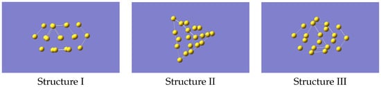
Figure 1.
Structures of Au used as starting geometries for generating data to train the machine learning potential.
Molecular Dynamics calculations were then performed on each structure to generate a series of geometries and their associated forces to parameterise the force field. We used Density Functional Theory (DFT) calculations within the framework of the Vienna Ab Initio Simulation Package (VASP) [27,28]. The projector augmented-wave (PAW) potentials are used to describe the core–valence interaction, with the valence electrons described by periodic plane waves with cut-off energy of 520 eV. The cubic supercell with lattice parameter of 30 Å contains the 20-atom clusters of the three structures. We used the generalized gradient approximation (GGA) for the exchange–correlation functional as formulated by Perdew-Burke-Ernzerhof (PBE) [29]. The energy and forces tolerance for structural relaxation are 10 eV and 10 eVÅ respectively. Equations of motion were integrated using the velocity Verlet algorithm, with a time step of 2.5 fs. The temperature of the system was stabilized using a Nosé–Hoover thermostat with the temperature-damping parameter of 10 time steps. The Nosé-Hoover thermostat is a deterministic method (no random forces or velocities) that is based on the extended system idea, in which an additional degree of freedom s is introduced to represent the thermal reservoir, which ensure an ergodicity within the canonical ensemble [30].
The data in the required format (energies, forces, geometries) is extracted from the VASP OUTCAR file using the DeePMD module dpdata [31]. This data is randomly split into training and validation sets in the ratio of 80:20. The DeePMD training program dp is run on the training set using the descriptor se_e2_a and parameters based on those provided in the DeePMD examples [31]. This process can be run on all the structures individually or all combined.
3. Results and Discussion
3.1. Generating the Data
Using VASP molecular dynamics simulations, we collected data for a maximum of ∼8500 timesteps for structure I and to ∼7500 for structure II and III, corresponding to 21,250 fs, and 18,750 fs respectively. The quality of the simulation is indicated by the excellent conservation of the constant of motion and the negligible drift in the fictitious kinetic energy of the electrons for simulations of that duration (Figure 2). The average temperature is ∼800 K for each structure, and the relatively large deviation due to the coupling with the Nosé thermostat, ensure an extensive sampling over the potential energy surface at large atomic distances (see Table 1). The large temperature fluctuations, indicated in Figure 2 and Table 1 correspond to a large nuclei’s velocities which lead to a large fluctuations in atomic distances during the simulations, ensuring an extensive sampling over the potential energy surface at large atomic distances. Table 1 reports the statistical analysis of the temperature distribution over time, indicating the amount of simulation-time where the system is away from the average temperature.
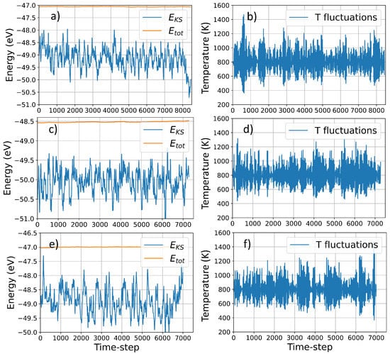
Figure 2.
Temperature and energy (potential vs total) fluctuations during VASP MD simulation structure I, II and III, In the figure, E and E indicate the electronic energy and total energy, respectively, whereas T fluctuations indicate the temperature fluctuations during the simulations due to the Nosé thermostat coupling. Panel (a) and (b), (c) and (d), and (e) and (f) correspond to structure I, II and III, respectively.

Table 1.
Statistical analysis of thermal fluctuations in VASP MD simulations.
A low average energy and small deviation during the simulation suggest the larger stability of structure II compared to the other configurations (see Table 2).
Table 2.
Statistical analysis of energy fluctuations in VASP MD simulations.
3.2. Evaluating the Potential
The training procedure in DeepMD reports RMS errors on both the force and the energy for the training and validation sets. The errors reported were similar for both training and validation, meaning that any overfitting had been avoided. The resulting potential from the training was tested on the validation set. Not all structures could be represented equally well. For example, for structure I, using the potential trained only on the energies and forces resulting from calculations on structure I, taking 1000 random points from the validation set produces the following results:
and plotted in Figure 3.
| #1000 points randomly chosen from the validation set | |||
| #DEEPMD INFO | # number of test data: 1000 | ||
| #DEEPMD INFO | Energy RMSE | : 8.219273e-02 eV | |
| #DEEPMD INFO | Energy RMSE/Natoms | : 4.109637e-03 eV | |
| #DEEPMD INFO | Force RMSE | : 6.739765e-02 eV/A | |
| #DEEPMD INFO | Virial RMSE | : 3.285809e+00 eV | |
| #DEEPMD INFO | Virial RMSE/Natoms | : 1.642904e-01 eV | |
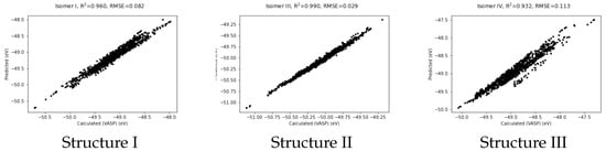
Figure 3.
Predicted vs VASP-calculated energies (in eV) for structures I, II and III.
It shows quite a good fit with RMSE of 0.082 eV and a coefficient of determination, R, of 0.960. The correlation plots for structures II and III also given in the Figure. These figures were produced using potentials obtained by training only on data from structure II and structure III respectively. Note that the fit for structure II is the best of the three. This may be because structure II closely resembles the pyramidal form of Au which is the global minimum and more rigid than the others.
It is possible to use all the data simultaneously and train to produce a more general potential which can describe all three structures. The fit for all structures trained simultaneously is shown in Figure 4a. The fit remains excellent with an R coefficient of 0.975, which is not quite as good as structure II on its own but bear in mind this covers a larger conformation space. A scatter plot (Figure 4b) of the errors in the energy shows that the vast majority of the errors are between ±0.1 eV but there are a few outliers deviating by as much as 0.4 eV.
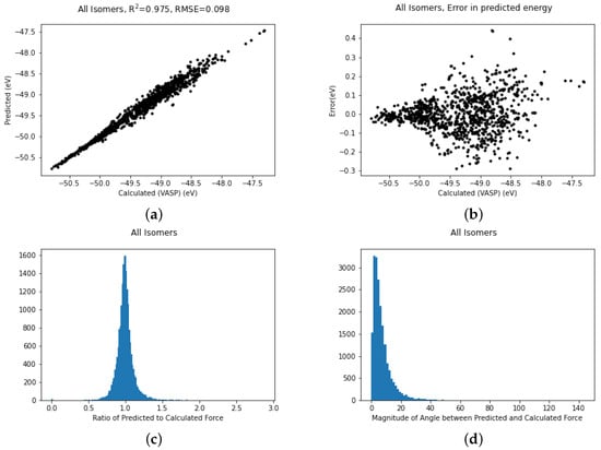
Figure 4.
Plots of (a) Fits of energies, (b) scatter in energy error, (c) error in magnitude of forces and (d) error in direction of forces for all the gold cluster structures trained simultaneously.
In molecular dynamics the forces are as important as the energy. Most machine learning studies in the area of potential fitting tend to discuss the energy more than the forces but as we believe the accuracy of the forces is meaningful we also include these graphs (Figure 4c,d). Figure 4c gives the ratio of the magnitude of the predicted force to the VASP-calculated force. In an ideal world this would be unity. Looking at the graph it is reassuringly very strongly peaked at 1. Furthermore, the magnitude of the angle between the computed and the predicted force, which should be zero, is similarly strongly peaked at zero. There are a small number of forces which have an error in angle greater than 100 degrees but these are too rare to show up in the histogram.
The most basic test for a potential is what it predicts as the minimum energy structure. To do this we compared the structures as predicted by a geometry optimisation in VASP with the 0K equilibrium structures as predicted by LAMMPS [32] using the machine learned potentials (Figure 5). The VASP minimum energy structures, starting from the initial structure described above, are in Figure 6.
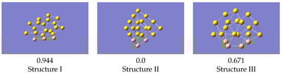
Figure 5.
LAMMPS optimised structures using the machine learned potential. Energies (in eV) given relative to the lowest energy structure.
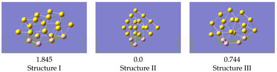
Figure 6.
VASP optimised structures from a regular VASP geometry optimisation. Energies (in eV) given relative to the lowest energy structure.
Structure II is the global minimum structure. The coordinates of these final structures are also given in the Supplementary Information. Relative to the pyramidal structure, structure III is 0.744 eV higher, and structure I 1.845 eV higher.
For the structures produced by LAMMPS, structure II again optimises to the global minimum, and structure III gives a geometry the same as VASP. Isomer I, from the same starting geometry as used with VASP, optimises to a structure very similar to VASP’s local minimum, but with a smaller energy difference relative to the ground state. Structure III is now 0.671 eV above the global minimum, which is in reasonable agreement with the VASP result. These results were all obtained with a potential derived using data from all structures simultaneously, i.e the one whose statistics are shown in Figure 4. Cao et al. [23] studied structures of several small gold clusters including Au, and found a local minimum which resembles the one shown here. Ford et al. [15] also found a similar structure at approximately the same energy above the global minimum.
3.3. Using the Potential
We computed the vibrational density of states from the velocity auto-correlation function in the three structures (see Figure 7). Each spectrum shows a single pronounced peak at ∼1–1.5 THz, reproducing one of the main peaks measured experimentally. This is due to the small size of the nanoparticle considered here, that favours low frequency phonon modes due to the large surface-bulk ratio, as suggested by Bertoldi et al. [33]. However, here we focus on the accuracy of DeePMD models in reproducing ab-initio calculations, and the absence of high frequency phonon modes is a negligible detail.
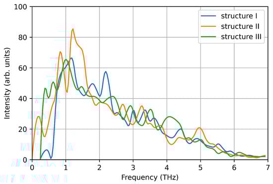
Figure 7.
Vibrational density of states computed from the velocity auto-correlation function in VASP simulations.
Using the energy fluctuation of the system with respect to the temperature described by Labastie et al., we calculated the heat capacity as follows [34]:
where E is the energy of the system, is the Boltzmann constant and T is the average temperature.
Using equation Equation (1), the specific heat capacity has been calculated using time windows of 2000 steps starting from different points of MD simulations. For structure II, value oscillates between 33.89 J/K/mol, or 0.34 meV/K/Atom, and 36.66 J/K/mol, or 0.38 meV/Atom (around 10%), with an average of 35.12 J/K/mol or 0.36 meV/K/Atom. Similar results are obtained for structure I and III with a relatively larger fluctuation in the values (around 20%) and the results are summarized in Table 3.
Table 3.
Specific heat capacity (C) at 800 K calculated using equation Equation (1) for VASP and LAMMPS simulations (values are given in J/K/ mol).
The specific heat values are higher than the corresponding bulk and decrease with the size of the nanoparticle [35]. Also, a second high peak frequency becomes less pronounced for small cluster size [36]. The literature report values of C 30, when calculated by modified tight-binding second-moment approximation [37], and ∼16.6 J/K/mol when calculated by Density Functional based Tight Binding method [38]. Small fluctuations in the value during the ab-initio simulation timeline, confirm the ergodicity of the systems, and the small deviation from the experimental value indicate the accuracy of the simulations.
When C is calculated by frozen phonon models in (1 × 1 × 1) expansion of the supercell. Due to the low symmetry of the clusters, the 126 single point calculations needed to evaluate the require CPU Time: 01:00:57. However, the value obtained is one order of magnitude larger (∼450–500 J/K/mol), due to the presence of intense fictitious low frequency phonon modes. The large error may be partially recovered using a larger expansion of the supercell, which, however, will lead to a very heavy calculation due to the low symmetry configuration of the clusters. The phonon DOS is included in the Supplementary Information.
Using the DeePMD calculated interatomic potentials, we repeat the nanocluster molecular dynamics with the same setup used for VASP MD. We use the interatomic potentials extrapolated by using all the three structures as training/test sets, which naturally include a generalised description of the of the energy surface. The deviation from average values of temperature and energy are comparable to the ones calculated in VASP MD for the same structure within 0.25% for the temperature and 6% for the energy, respectively (see Figure 8 and Table 4). The calculated value using energy fluctuations is around 40% smaller that the ones calculated using VASP. However, this deviation is comparable with the distribution of values using different theoretical/computational approaches reported in the literature [37,38]. Furthermore, the vibrational DOS calculated using ML-IP, reproduce the low frequency peak calculated by VASP MD (see Figure 9).
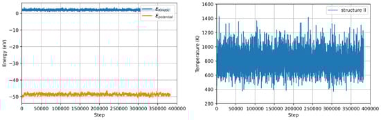
Figure 8.
Energy (potential vs total) (left panel) and Temperature (right panel) fluctuations during LAMMPS MD simulation structure II.
Table 4.
Statistical analysis of energy fluctuations in structure II during LAMMPS MD simulations.
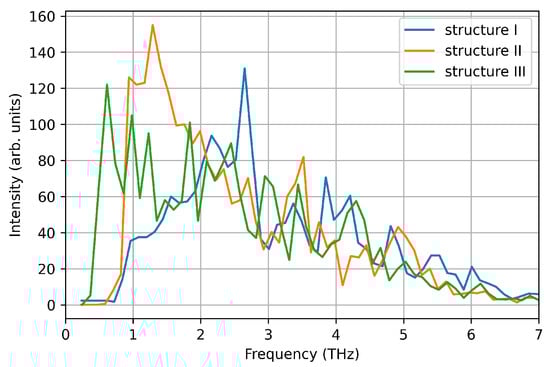
Figure 9.
Vibrational density of states computed from the velocity auto-correlation function in LAMMPS simulations.
The computational time necessary for a simulation to reach 8500 timesteps using VASP is (CPU Time: 10,301:11:16) on 48 CPUs, whereas the same number of timesteps uses only (CPU Time: 00:03:20) on 4 CPUs using the Machine Learning Potential in LAMMPS, confirming the huge resource-wise benefit of ML approach if compared to conventional quantum mechanical models, preserving accuracy.
4. Conclusions
Using the DeePMD program we have shown that Machine Learned potentials are a feasible way of calculating the properties of gold nanoclusters at similar accuracy but reduced computational cost to standard ab-initio molecular dynamics methods. Our potential correctly reproduces the global minimum of Au and one of the local minima. We have calculated the heat capacity using both ab-initio and machine-learned MD and they agree satisfactorily with each other and related studies from the literature. In the course of the investigation further scope for improvement became apparent, such as reducing the number of data points while retaining accuracy, using alternative methods to generate the training data, better descriptors for the ML model and so on. These are currently under investigation. In particular, recent works [20,39] using new techniques that build on and enhance existing data to produce more general data, such as in active or delta learning, look promising for future work.
Supplementary Materials
The following supporting information can be downloaded at: https://www.mdpi.com/article/10.3390/nano12213891/s1, Table S1: Initial geometry of structure I, Table S2: Initial geometry of structure II, Table S3: Initial geometry of structure III, Table S4: Geometry of structure I optimised by VASP, Table S5: Geometry of structure II optimised by VASP, Table S6: Geometry of structure III optimised by VASP, Table S7: Geometry of structure I optimised by LAMMPS, Table S8: Geometry of structure II optimised by LAMMPS, Table S9: Geometry of structure III optimised by LAMMPS, Figure S10: Phonon Density of States computed with the frozen phonon model. Example of the training parameters used in the DeePMD fitting of the potential.
Author Contributions
All authors contributed to the planning and design of the final project. Conceptualisation, R.K., R.D.A., K.W., N.M. and R.K.M.; Preliminary investigation, K.W., N.M. and R.K.M.; Further investigation, M.F. and R.D.A.; All authors contributed to the writing of the manuscript; writing—original draft preparation, R.K., M.F. and R.D.A.; writing—review and editing, all authors. All authors have read and agreed to the published version of the manuscript.
Funding
This research was funded by the Australian Government through the Australian Research Council (ARC DP200101217).
Institutional Review Board Statement
Not applicable.
Informed Consent Statement
Not applicable.
Data Availability Statement
Coordinates of the structures used in this study are provided in the Supplementary Information.
Acknowledgments
The authors would like to thank Mike Ford, Tim Duignan and David Reith for helpful discussions. The authors gratefully acknowledge the financial support of Australian Government through the Australian Research Council (ARC DP200101217). The theoretical calculations in this research were undertaken with the assistance of resources from the National Computational Infrastructure (NCI), which is supported by the Australian Government. The theoretical calculations in this work were also supported by resources provided by the Pawsey Supercomputing Centre.
Conflicts of Interest
The authors declare no conflict of interest.
References
- Mueller, T.; Hernandez, A.; Wang, C. Machine learning for interatomic potential models. J. Chem. Phys. 2020, 152, 050902. [Google Scholar] [CrossRef] [PubMed]
- Mishin, Y. Machine-learning interatomic potentials for materials science. Acta Mater. 2021, 214, 116980. [Google Scholar] [CrossRef]
- Senftle, T.; Hong, S.; Islam, M.; Kylasa, S.B.; Zheng, Y.; Shin, Y.K.; Junkermeier, C.; Engel-Herbert, R.; Janik, M.J.; Aktulga, H.M.; et al. The ReaxFF reactive force-field: Development, applications and future directions. Npj Comput. Mater. 2016, 2, 15011. [Google Scholar] [CrossRef]
- Gissinger, J.R.; Jensen, B.R.; Wise, K.E. Modeling chemical reactions in classical molecular dynamics simulations. Polymer 2017, 128, 211–217. [Google Scholar] [CrossRef] [PubMed]
- Behler, J. Perspective: Machine learning potentials for atomistic simulations. J. Chem. Phys. 2016, 145, 170901. [Google Scholar] [CrossRef] [PubMed]
- Zuo, Y.; Chen, C.; Li, X.; Deng, Z.; Chen, Y.; Behler, J.; Csányi, G.; Shapeev, A.V.; Thompson, A.P.; Wood, M.A.; et al. Performance and Cost Assessment of Machine Learning Interatomic Potentials. J. Phys. Chem. A 2020, 124, 731–745. [Google Scholar] [CrossRef]
- Wang, H.; Zhang, L.; Han, J.; Weinan, E. DeePMD-kit: A deep learning package for many-body potential energy representation and molecular dynamics. Comp. Phys. Comm. 2018, 228, 178–184. [Google Scholar] [CrossRef]
- DeepModeling. Available online: https://deepmodeling.com (accessed on 12 August 2022).
- MedeA Software. Available online: https://www.materialsdesign.com/medea-software (accessed on 8 December 2021).
- Seko, A.; Togo, A.; Tanaka, I. Group-theoretical high-order rotational invariants for structural representations: Application to linearized machine learning interatomic potential. Phys. Rev. B 2019, 99, 214108. [Google Scholar] [CrossRef]
- Deringer, V.L.; Pickard, C.J.; Csàanyi, G. Data-driven learning of total and local energies in elemental boron. Phys. Rev. Lett. 2018, 120, 156001. [Google Scholar] [CrossRef]
- Kolsbjerg, E.L.; Peterson, A.A.; Hammer, B. Neural-network-enhanced evolutionary algorithm applied to supported metal nanoparticles. Phys. Rev. B 2018, 97, 195424. [Google Scholar] [CrossRef]
- Caro, M.A.; Aarva, A.; Deringer, V.L.; Csányi, G.; Laurila, T. Reactivity of amorphous carbon surfaces: Rationalizing the role of structural motifs in functionalization using machine learning. Chem. Mater. 2018, 30, 7446–7455. [Google Scholar] [CrossRef] [PubMed]
- Zhang, J.; Pagotto, J.; Duignan, T.T. Perspective: Towards predictive design of electrolyte solutions by accelerating ab initio simulation with neural networks. J. Mat. Chem. A 2022, 10, 19560–19571. [Google Scholar] [CrossRef]
- Krishnamurty, S.; Shafai, G.S.; Kanhere, D.G.; de Bas, B.S.; Ford, M.J. Ab Initio Molecular Dynamical Investigation of the Finite Temperature Behavior of the Tetrahedral Au19 and Au20 Clusters. J. Phys. Chem. A 2007, 111, 10769–10775. [Google Scholar] [CrossRef] [PubMed]
- Kamiński, M.; Jurkiewicz, K.; Burian, A.; Bródka, A. The structure of gold nanoparticles: Molecular dynamics modeling and its verification by X-ray diffraction. J. Appl. Cryst. 2020, 53, 1–8. [Google Scholar] [CrossRef]
- Astruc, D. (Ed.) Nanoparticles in Catalysis [Special issue]. Chem. Rev. 2020, 120, 461–463. [Google Scholar] [CrossRef] [PubMed]
- Ishida, T.; Murayama, T.; Taketoshi, A.; Haruta, M. Importance of Size and Contact Structure of Gold Nanoparticles for the Genesis of Unique Catalytic Processes. Chem. Rev. 2020, 120, 464–525. [Google Scholar] [CrossRef]
- Zeni, C.; Rossi, K.; Pavloudis, T.; Kioseoglou, J.; de Gironcoli, S.; Palmer, R.E.; Baletto, F. Data-driven simulation and characterisation of gold nanoparticle melting. Nat. Commun. 2021, 12, 6056. [Google Scholar] [CrossRef]
- Loeffler, T.D.; Manna, S.; Patra, T.K.; Chan, H.; Badri Narayanan, B.; Sankaranarayanan, S. Active Learning A Neural Network Model for Gold Clusters & Bulk From Sparse First Principles Training Data. ChemCatChem 2020, 12, 4699. [Google Scholar]
- Ouyang, R.; Xie, Y.; Jiang, D. Global minimization of gold clusters by combining neural network potentials and the basin-hopping method. Nanoscale 2015, 7, 14817–14821. [Google Scholar] [CrossRef]
- Thorn, A.; Rojas-Nunez, J.; Hajinazar, S.; Baltazar, S.E.; Kolmogorov, A.N. Toward ab Initio Ground States of Gold Clusters via Neural Network Modeling. J. Phys. Chem. C 2019, 123, 30088–30098. [Google Scholar] [CrossRef]
- Cao, L.; Guo, Y.; Han, W.; Xu, W.; Sai, L.; Fu, J. Artificial neural network potential for Au20 clusters based on the first-principles. J. Phys. Condens. Matter 2022, 34, 174005–174012. [Google Scholar] [CrossRef] [PubMed]
- Abadi, M.; Agarwal, A.; Barham, P.; Brevdo, E.; Chen, Z.; Citro, C.; Corrado, G.S.; Davis, A.; Dean, J.; Devin, M.; et al. TensorFlow: Large-Scale Machine Learning on Heterogeneous Systems. Software. 2015. Available online: tensorflow.org (accessed on 15 August 2022).
- Bartók, A.P.; Kondor, R.; Csányi, G. On representing chemical environments. Phys. Rev. B 2013, 87, 184115. [Google Scholar] [CrossRef]
- Khetrapal, N.S.; Bulusu, S.S.; Zeng, X.C. Structural Evolution of Gold Clusters (n = 21–25). J. Phys. Chem. 2017, 121, 2466–2474. [Google Scholar] [CrossRef] [PubMed]
- Kresse, G.; Hafner, J. Ab initio molecular dynamics for liquid metals. Phys. Rev. B 1993, 47, 558. [Google Scholar] [CrossRef] [PubMed]
- Kresse, G.; Furthmüller, J. Efficient iterative schemes for ab initio total-energy calculations using a plane-wave basis set. Phys. Rev. B 1996, 54, 11169. [Google Scholar] [CrossRef] [PubMed]
- Perdew, J.P.; Burke, K.; Ernzerhof, M. Generalized Gradient Approximation Made Simple. Phys. Rev. Lett. 1996, 77, 3865. [Google Scholar] [CrossRef] [PubMed]
- Nosé, S. A unified formulation of the constant temperature molecular dynamics methods. J. Chem. Phys. 1984, 81, 511–519. [Google Scholar] [CrossRef]
- DeepModeling Documentations. Available online: https://docs.deepmodeling.com (accessed on 12 August 2022).
- Thompson, A.P.; Aktulga, H.M.; Berger, R.; Bolintineanu, D.S.; Brown, W.M.; Crozier, P.S.; in’t Veld, P.J.; Kohlmeyer, A.; Moore, S.G.; Nguyen, T.D.; et al. LAMMPS—A flexible simulation tool for particle-based materials modeling at the atomic, meso, and continuum scales. Comp. Phys. Comm. 2022, 271, 10817. [Google Scholar] [CrossRef]
- Bertoldi, D.S.; Guillermet, A.F. Systematics of vibrational properties of Au nanoparticles: A molecular dynamics approach. Phys. Chem. Chem. Phys. 2022, 24, 21833–21840. [Google Scholar] [CrossRef]
- Labastie, P.; Whetten, R.L. Statistical thermodynamics of the cluster solid-liquid transition. Phys. Rev. Lett. 1990, 65, 1567. [Google Scholar] [CrossRef]
- Bhatt, S.; Kumar, R.; Kumar, M. Specific heat and thermal conductivity of nanomaterials. Mod. Phys. Lett. B 2017, 31, 1750011. [Google Scholar] [CrossRef]
- Sauceda, H.E.; Salazar, F.; Pérez, L.A.; Garzón, I.L. Size and shape dependence of the vibrational spectrum and low-temperature specific heat of Au nanoparticles. J. Phys. Chem. C 2013, 117, 25160–25168. [Google Scholar] [CrossRef]
- Gafner, Y.; Gafner, S.L.; Zamulin, I.S.; Redel, L.V.; Baidyshev, V.S. Analysis of the heat capacity of nanoclusters of FCC metals on the example of Al, Ni, Cu, Pd, and Au. Phys. Met. Metallogr. 2015, 116, 568–575. [Google Scholar] [CrossRef]
- Rapacioli, M.; Tarrat, N.; Spiegelman, F. Melting of the Au20 gold cluster: Does charge matter? J. Phys. Chem. A 2018, 122, 4092–4098. [Google Scholar] [CrossRef]
- Liu, P.; Verdi, C.; Karsai, F.; Kresse, G. Phase transitions of zirconia: Machine-learned force fields beyond density functional theory. Phys. Rev. B 2022, 105, L060102. [Google Scholar] [CrossRef]


Publisher’s Note: MDPI stays neutral with regard to jurisdictional claims in published maps and institutional affiliations. |
© 2022 by the authors. Licensee MDPI, Basel, Switzerland. This article is an open access article distributed under the terms and conditions of the Creative Commons Attribution (CC BY) license (https://creativecommons.org/licenses/by/4.0/).